LS-SVM Functional Network for Time Series Prediction - UCL/ELEN

ESANN'2006 proceedings - European Symposium on Artificial Neural Networks Bruges (Belgium), 26-28 April 2006, d-side publi., ISBN 2-930307-06-4.

LS-SVM Functional Network for Time Series Prediction Tuomas K¨ arn¨ a1 , Fabrice Rossi2 and Amaury Lendasse1 Helsinki University of Technology - Neural Networks Research Center P.O. Box 5400, FI-02015 - Finland 2- Projet AxIS, INRIA, Domaine de Voluceau, Rocquencourt, B.P. 105 78153 Le Chesnay Cedex - France Abstract. Usually time series prediction is done with regularly sampled data. In practice, however, the data available may be irregularly sampled. In this case the conventional prediction methods cannot be used. One solution is to use Functional Data Analysis (FDA). In FDA an interpolating function is fitted to the data and the fitting coefficients are being analyzed instead of the original data points. In this paper, we propose a functional approach to time series prediction. Radial Basis Function Network (RBFN) is used for the interpolation. The interpolation parameters are optimized with a k-Nearest Neighbors (k-NN) model. Least Squares Support Vector Machine (LS-SVM) is used for the prediction.

1

Introduction

Time series prediction [1] is an important part of decision making in many application domains such as climatology and electricity network management. Usually linear models or neural network based methods are used for this task. Past values are used as inputs to the model and the output provides an estimate for the next value. These methods, however, have a serious limitation: the time series must be regularly sampled. In some application fields, such as medical time series, irregular sampling is frequent. Moreover, missing data are common in many real world application and correspond to a particular case of irregular sampling. In those cases conventional methods cannot be used. One solution is to regenerate constantly sampled data by resampling the original data. This approach, however, is fairly noisy and thus not recommended. A better idea is to use Functional Data Analysis (FDA) [2]. In FDA the problem is casted into some function space where it can be analyzed more efficiently. This approach is based on the assumption that the data points are samples of some continuous function. The unknown function is estimated using some regression technique and the estimate is used as an input to the model. Neural networks that process functional data are called functional networks. They have been successfully applied to various data analysis tasks (see for example [6]). In this paper, we introduce a functional time series prediction method inspired by functional auto-regressive model [3]. First a Radial Basis Function Network regressor is fitted to the data in time space. The fitting coefficients (i.e. weights of the RBF) are used as training examples for a Least Squares Support Vector Machine (LS-SVM) [4] prediction model.

473

ESANN'2006 proceedings - European Symposium on Artificial Neural Networks Bruges (Belgium), 26-28 April 2006, d-side publi., ISBN 2-930307-06-4.

The concept of functional networks is discussed in Section 2. In Section 3 the LS-SVM is presented briefly and in Section 4 the prediction method is outlined. An application to real world data is presented in Section 5.

2

Functional Networks

Functional networks stand for neural networks that process functional data instead of Rn data, using principals from Functional Data Analysis [2] For more detailed information about functional networks see for instance [6] and [8]. In literature functional data has been successfully applied to some neural networks models, mainly Radial Basis Function Networks (RBFN) and Multilayer Perceptrons (MLP) [6]. FDA can be considered as an extension to traditional data analysis. Multivariate analysis consists mainly of just vector operations, including norm and inner product. However, these operations are available on any Hilbert space and thus also on some function spaces such as L2 . Therefore much of the developed data analysis theory can be applied directly on functional data. In practice functional data are never directly available: each function is known via a set of (input, output) pairs, possibly corrupted by noise. The first step is to try to estimate these underlying functions by projecting the data on some functional basis. Since function spaces in general are infinite dimensional, the basis must be truncated (as in the case of Fourier transform) or some approximation must be applied (as in the case of b-splines). Let us assume that we have N observations and each observation consists of i p i i mi pairs of measurements (xij , yji )m j=1 , where xj ∈ R , yj ∈ R and i = 1, . . . , N . Basic assumption of FDA is that there is a regular function fi ∈ L2 such that yji = fi (xij ) + sij , where sij stands for the observation noise. Knowing the truncated basis ϕi of the finite-dimensional function space A we can approximate fi by minimizing the training error, min J(wi ) =

mi  

2

yji − fˆi (xij )

with fˆi (x) =

j=1

q 

wi,l ϕl (x),

l=1

where wi,l are the fitting coefficients and q is the dimension of A. The function fˆi is uniquely defined by the numerical regression coefficients wi = [wi,1 , wi,2 , . . . , wi,q ]T . Since the basis functions are not usually orthonormal (think to B-splines for instance) we transform the coefficients according to ω i = Uwi where U is the Choleski decomposition Φ = UT U of the matrix Φi,j = ϕi , ϕj . Euclidean operations (e.g., scalar product) on the transformed coefficients are equivalent to the corresponding operations in the functional space [6] (e.g. functional inner product): once the function estimates ω i have been obtained any conventional neural network model can be used for analysis.

474

ESANN'2006 proceedings - European Symposium on Artificial Neural Networks Bruges (Belgium), 26-28 April 2006, d-side publi., ISBN 2-930307-06-4.

3

LS-SVM for regression

LS-SVM is a least squares modification to the Support Vector Machine (SVM) [4]. The major advantage of LS-SVM is that it is computationally very cheap while it still possesses some important properties of the SVM. In this section we will briefly discuss the LS-SVM method for a regression task. For more detailed information see [4]. Again assume that we have a set of examples (xi , yi )N i=1 and the goal is to estimate a function f as mentioned in the previous section. Basically we define a N dimensional function space by defining the mappings ϕ = [ϕ1 , ϕ2 , . . . , ϕN ]T according to the measured points. The LS-SVM model is of the form fˆ(x) = wT ϕ(x) + b where w is a weight vector and b is a bias term. The optimization problem is the following, N

min J(w, ) = so that

yi

=

1 T 1 2 w w+γ  2 2 i=1 i wT ϕ(xi ) + b + i ,

i = 1, . . . , N

where the fitting error is denoted by i . Hyper-parameter γ controls the trade-off between the smoothness of the function and the accuracy of the fitting. This optimization problem leads to a solution, fˆ(x) =

N 

αi K(x, xi ) + b

i=1

where αi are the coefficients and K(x, xi ) = ϕT (x)ϕ(xi ) is the kernel. A common choice for the kernel is the Gaussian RBF, K(x, xi ) = e−

4 4.1

x − xi 2 . 2σ 2

Time Series Prediction with Functional Network Methodology

Consider a time series {ti , yi }N i=1 where the time stamps ti belong to a closed interval [a, b]. First the data is divided into input windows Ih and output windows Oh , with h = 1, . . . , (b − a − 2L)/δ + 1: Ih

=

{(ti , yi ) | a + (h − 1)δ

Oh

=

{(ti , yi ) | a + (h − 1)δ + L ≤ ti < a + (h − 1)δ + 2L}.

≤ ti < a + (h − 1)δ + L},

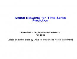
All windows have the same length L on the time axis. The shift between two sequential windows is δ. In the case of regularly sampled data the sampling interval is a natural choice for δ. A outline if the prediction schema is shown in Figure 1. On each window, the time series is considered as a function and is modelled by a RBF network

475

ESANN'2006 proceedings - European Symposium on Artificial Neural Networks Bruges (Belgium), 26-28 April 2006, d-side publi., ISBN 2-930307-06-4.

Input (ti,yi)

Output

Coefficients RBF with regularization



LS-SVM

Fig. 1: Prediction method. First a RBF regressor is fitted to the data points. The prediction in done in the function space using LS-SVM. Thus the output is also a set of coefficients. with Gaussian kernels. The centers of the kernels are equally distributed on an interval 10 per cent wider than the window. This ensures that the function fˆ can be monotonically increasing at the borders of the window. In other words the model is q  wi K(t, ti ), f˜(t) = i=1

where ti are the fixed centers and q is the number of kernels. Furthermore a regularization term wT w is used in the fitting to prevent overfitting [5]. The fitting coefficients are transformed using the Choleski decomposition as mentioned in Section 2. The obtained sets of input and output coefficients are denoted as Ih = ω(Ih ) and Oh = ω(Oh ) respectively. Finally a prediction mapping P : Ih → Oh in the function space is trained with LS-SVM. The kernel is also a Gaussian RBF. Since the dimension of the output is q, we are actually training q separate LS-SVM regressors for each dimension. The performance of the prediction is evaluated in a separate validation set. The mean square error at the known data locations is used as an error measure. 4.2

Optimizing parameters

There are basically four unknown parameters involved in the window function fitting: the window length L, number of kernels q, width of the kernels σ and the regularization parameter γ. These parameters are optimized with a grid search. A predefined set of values is tested for each parameter. The parameter combination with the smallest Leave One Out (LOO) error is selected. Because we are exploring a four dimensional grid it is essential to speed up the testing process. For this purpose the fitting parameters are optimized using a k-NN approximator [7] [5] instead of LS-SVM. Since k-NN is computationally a very cheap method one is able to perform an larger search that would be feasible with LS-SVM. Of course the drawback is that the obtained parameters may not be optimal for the LS-SVM model. Once the best fitting parameters are found a LS-SVM model is trained. The LS-SVM introduces two more unknown parameters γ˜ and σ ˜ . These parameters are also optimized with a grid search using LOO error.

476

ESANN'2006 proceedings - European Symposium on Artificial Neural Networks Bruges (Belgium), 26-28 April 2006, d-side publi., ISBN 2-930307-06-4.

5

Time Series prediction Application

5.1

Darwin dataset

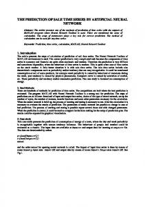
The proposed prediction schema was tested with the Darwin dataset. It contains monthly values of sea level air pressures measured between years 1882 and 1998. An example of the data is shown in Figure 2 a). The first 1300 values of total 1400 were used for training and the remaining 100 values were used for validation. Darwin dataset is constantly sampled. To experiment with missing data we randomly removed 33 per cent of the data points in the training set. In this experiment the mean square error was evaluated only in the first available data point. b)

a) 16

15 14

14

13 12

12

Y

Y

11 10

10 9

8

8 7 6

6 4 300

320

340

360

380

400

420

440

460

480

5 1270

500

1280

Time

1290

1300

1310

1320

1330

Time

Fig. 2: a) Darwin dataset. b) Example of prediction.

5.2

Results

We performed several grid searches with k-NN model to tune the four fitting parameters. Figure 2 b) shows and example of the prediction with the best model (See Table 1). On the left there are the input data points and the input function while the correct output function and corresponding data points are on the right. The predicted output is marked with a solid line. A LS-SVM model was trained using these parameters. For reference the k-NN prediction was tested also without any data loss. The results are shown in Table 2. L 27.1

q 8

σ 1.70

γ 348

k 25

Table 1: The best parameter setup for k-NN prediction with 33 % dataloss. First of all it should be noted that the k-NN performance is very good when no data has been removed. Only the best conventional methods can reach better

477

ESANN'2006 proceedings - European Symposium on Artificial Neural Networks Bruges (Belgium), 26-28 April 2006, d-side publi., ISBN 2-930307-06-4.

LOO error Test error

k-NN 0 % dataloss 33 % dataloss 0.83 1.19 0.96 1.49

LS-SVM 33 % dataloss 1.15 1.39

Table 2: Results of the Darwin dataset. This table contains mean square prediction errors on the learning set (LOO) as well as on the test set. k-NN was experimented with both 0 per cent and 33 per cent dataloss. Using the best setup of the latter case a LS-SVM model was trained. mean square error. Naturally the error increases when one third of data is removed, but not so much as one would intuitively expect. Furthermore it can be seen that the LS-SVM model performs clearly better than k-NN.

6

Conclusions

We have proposed a functional LS-SVM time series prediction method to deal with the problem of irregular sampling or missing data. The method was experimented with the Darwin dataset. The results obtained with no data loss show that the functional approach is entirely comparable to the conventional methods. Furthermore the prediction performs reasonably well even if one third of the data points are missing. In future, more tests should be done with irregularly sampled data.

References [1] A. Weigend and N. Gershenfeld, editors. Time Series Prediction: Forecasting the Future and Understanding the Past, Addison-Wesley, Reading (MA), 1994. [2] J. Ramsay and B. Silverman. Functional Data Analysis, Springer Series in Statistics, Springer Verlag, 1997. [3] Besse, P., Cardot, H., Stephenson, D., 2000. Autoregressive forecasting of some functional climatic variations. Scandinavian Journal of Statistics 4, 673–688. [4] J. Suykens, T. Van Gestel, J. De Brabanter, B. De Moor and J. Vandewalle, Least Squares Support Vector Machines, World Scientific Publishing Co., Singapore, 2002. [5] C. Bishop, Neural Networks for Pattern Recognition, Oxford University Press, Clarendon, 1995 [6] F. Rossi, N. Delannay, B. Conan-Guez, M. Verleysen, Representation of functional data in neural networks Neurocomputing, 64:183-210, Elsevier, 2005. [7] A. Sorjamaa, N. Reyhani, A. Lendasse, Input and Structure Selection for k-NN Approximator. In J. Cabestany, A. Prieto, F. Sandoval, editors, proceedings of the 8th International Workshop on Artificial Neural Networks (IWANN 2005), Lecture Notes in Computer Science 3512, pages 985-991, Springer-Verlag, 2005. [8] B. Hammer and B. Jain, Neural Methods for non-standard data In M. Verleysen, editor, proceedings of the 12th European Symposium on Artificial Neural Networks (ESANN 2004), d-side pub., pages 281-292, April 28-30, Bruges (Belgium), 2004.

478