LS-SVR with Variant Parameters and its Practical Applications for Seismic Prospecting Data Denoising DENG Xiaoying a,b, YANG Dinghui a,YANG Baojun *b Department of Mathematics, Tsinghua University, Beijing, China 100084; b Department of Geophysics, Jilin University, Changchun, China 130026 E-mail:
[email protected] or
[email protected],
[email protected],
[email protected] a
Abstract-Signal denoising can be considered as a function regression problem. LS-SVR (Least Squares-Support Vector Regression) based on Ricker wavelet kernel function is applied to the practical seismic prospecting data denoising in this paper. To adapt LS-SVR well to the practical seismic data, the parameters including Ricker wavelet kernel parameter f and regularization parameter γ are selected automatically according to the features of data in the fixed window. The denoising experimental results for the theoretical and practical seismic data show that the performance of Ricker wavelet LS-SVR with variant parameters outperforms the one with invariant parameters in terms of the retrieved waveform in time domain and spectrum range in frequency domain. Index Terms-LS-SVR; Ricker wavelet kernel function; seismic prospecting event; variant parameters
Signal denoising can be considered as a function regression problem, which involves estimating the underlying relationship from detected signal data set[7]. Based on the former research results of authors[8,9], this paper applies LS-SVR with variant parameters to seismic prospecting data denoising so as to suppress the random noise. Firstly we select a fixed window, and then automatically select the parameters according to the features of data in the window. The experimental results for the theoretical and practical seismic data denoising show that the performance of Ricker wavelet LS-SVR with variant parameters outperforms the one with invariant parameters in terms of the retrieved waveform in time domain and spectrum range in frequency domain. II. LS-SVR AND RICKER WAVELET LS-SVR
I.
INTRODUCTION
SVM (Support Vector Machine) is a new universal learning machine based on principles of structure risk minimization and statistical learning theory[1] with superior generalization performance than conventional learning methods such as neural network. SVM generalization performance does not depend on the dimensionality of the input space because of using kernel mapping. So it has be applied widely to many fields such as classification, regression[2], textual recognition[3], face recognition[4], fault diagnosis[5] and time series prediction[6],etc. Bing-Yu Sun[7] applied it to signal denoising only aiming to Lidar signal under weak noise. SVM is named as SVR(Support Vector Regression) when applied to function regression. LS-SVM is SVM’s modified form for simplicity. In seismic prospecting for oil and gas, suppressing the random noise so as to improve the ratio of signal-to-noise (SNR) of seismic data is very important. Many kinds of denoising methods have been proposed including multicoverage technique which needs measuring the same object many time; singular value decomposition which is difficult to be computed in some cases; median filtering which needs good correlation; f-x prediction filtering, time-frequency analysis technique, KL transformation and so on.
978-1-4244-1666-0/08/$25.00 '2008 IEEE
Given a training data set of {( xi , y i ), i = 1,2, L, l} with input data xi ∈ R N and output data y i ∈ R . The optimization problem of LS-SVR with constraints in primal space is described by γ l 2 1 2 (1) min
w +
2
2
∑e
i
i =1
s.t. f ( xi ) = w T φ ( xi ) + b + ei , i = 1, L, l
where γ ∈ R is the regularization parameter, φ (x) is a nonlinear function that maps the input space into a higher dimensional feature space (possibly infinite-dimensional), w is the weight vector with the same dimensionality as feature space, b is a bias term and ei ∈ R is the error variant. Using Lagrange multipliers method in the dual space and solving a set of linear equations, we can get the function for regression as follows: l
f ( x) =
∑ α K ( x , x) + b i
i
(2)
i =1
where K ( xi , x) = φ ( xi ) ⋅ φ ( x) is called as kernel function according to Mercer’s theory, and α i (i = 1,2, L , l ) ∈ R is Lagrange multipliers. Kernel function plays an important role in SVM. It replaces the inner product in higher dimensional feature space to overcome the dimensional disaster. Now there are several kinds of kernel function often used including linear kernel, polynomial kernel and exponential radial basis function (RBF) kernel, etc. Because Ricker wavelet is often used to simulate the seismic
1060
Authorized licensed use limited to: IEEE Xplore. Downloaded on January 12, 2009 at 06:48 from IEEE Xplore. Restrictions apply.
wavelet in the theoretical analysis of seismic signal processing, Ref.[8] proposed and proved a permitted support vector kernel —Ricker wavelet kernel 2 −π f x − x ' . (3) K ( x, x' ) = (1 − 2π 2 f 2 x − x' )e where f ∈ R ( f > 0 ) is kernel parameter. Ricker wavelet LSSVR is superior to RBF kernel LS-SVR and Wiener filtering when applied to the noise reduction of seismic prospecting signals[8]. 2
1
2
10 channel
2
common shot data with 30 channels in accordance with the hyperbolic time-distance equation, shown as Fig.1 (a). Fig.1(b)
A
B
20
PARAMETERS SELECTION
where y and σ y are the mean and the standard deviation of the y values of training data. In the single channel of seismic prospecting data, because the predominant frequencies of the reflected seismic wavelets gradually decline as the recording time, and the selection of parameter f in Ricker wavelet LS-SVR is associated with the predominant frequency of signal, selecting variant parameter f as the different seismic wavelets is more suitable for the practical case. In order to keep the continuity of magnitude of the retrieved signal, regularization parameter γ is kept unchangeable in this paper. Generally, the duration of a seismic wavelet approximates 100ms, more or less, so we process 100 ms-length data every time. But 200 ms-length data centered on the 100 ms-length data are used to determine the values of parameter f by FFT for finding more appropriate parameter. If the noise in the selected window is very strong so that the predominant frequency detected by FFT falls away the range which it should fall in by a priori knowledge, parameter f is given as the mean of all f detected or an experiential value by a priori knowledge.
(a) 30 0
0.2
0.4
0.6
0.8
1
1.2
t/s 1
10 channel
A
B
20
(b) 30 0
0.2
0.4
0.6
0.8
1
1.2
t/s γ=1.6472 ,
f ( Ricker ) =17.4048
1
A
10
B
channel
LS-SVR embeds two tunable parameters including kernel parameter and regularization parameter that control the training setting, in which the later regulates the ratio between empirical risk and confidence interval of learning machine. These parameters may diminish the overall performance of LS-SVR if not well chosen. Ref.[9] investigated the selection problem of parameters of Ricker wavelet LS-SVR, and concluded that kernel parameter f should be set as predominant frequency of seismic signal, and the accepted range of regularization parameter γ is very wide. We select it by the means of Ref.[10].Cherkassky [10] proposed analytical selection directly from the training data and let (4) γ = max( y + 3σ y , y − 3σ y )
20
30 0
(c)
0.2
0.4
0.6
0.8
1
1.2
t/s γ=1.6472, f(variable), window length=100
1
A
B
10 channel
III.
(d)
20
IV. THEORETICAL SEISMIC DATA DENOISING SIMULATION EXPERIMENTS
Suppose that the velocities of two reflected wave events are v1=1800 m/s and v2=2000 m/s, the arrival times of their first channel are 0.1s and 0.8s, and their predominant frequencies are 30Hz and 15Hz, respectively. The sampling frequency is set as 1000Hz. Using Ricker wavelet, we synthesize the
30 0
0.2
0.4
0.6
0.8
1
1.2
t/s
Fig. 1 Theoretical seismic data denoising experiments (a) data without noise; (b) noisy data; (c) denoising result of LS-SVR; (d) denoising result of LS-SVR with variant parameters
1061 Authorized licensed use limited to: IEEE Xplore. Downloaded on January 12, 2009 at 06:48 from IEEE Xplore. Restrictions apply.
Fig.2. Obviously, the spectrum of LS-SVR loses some effective bands such as [40 60], while the spectrum of our proposed LS-SVR with variant parameters is closer to the spectrum of data without noise. From the above theoretical seismic data denoising simulation experiments, we can see that in both time domain and frequency domain, our proposed LS-SVR with variant parameters is superior to LS-SVR with invariant parameters. spectrum of data without noise 50 0
magnitude spectrum
shows the data corrupted by additive Gaussian white noise with variance σ 2 =0.1w. The noise in Fig.1(b) makes two events very faint, especially the event A with higher predominant frequency . We process the data channel by channel. Firstly, the data of every channel is divided into windows every 100 data points. Then select two parameters by the aforementioned way and select every other data point as the training set to apply Ricker wavelet LS-SVR. Lastly, compute all points by LS-SVR model obtained. Fig.1(c) shows the denoising result of LS-SVR with invariant parameters, where fixs parameter f =17.4048, the mean of the predominant frequencies of all channels detected by FFT, and fixs regularization parameter γ=1.6472 by the formula (4). Fig.1(d) shows the result of LS-SVR with variant parameter f and fixed parameter γ=1.6472. Note that when the predominant frequency found by FFT do not fall into the interval of [5 50], the parameter f is set as the same value with the previous method, i.e. 17.4048. Comparatively with the data without noise in Fig.1(a), the wavelet of event A in Fig.1(c) becomes ‘fat’, that is to say, its frequency becomes lower. The reason is that the kernel parameter f is selected incorrectly. However, the one in Fig.1(d) is almost unchangeable at the cost of bringing a little high-frequency noise. The event B in Fig.1(d) is also better than the one in Fig.1(c) from the continuity of event and similarity with Fig.1(a). Select an arbitrary channel of data and analyze its spectrum showed as
0
20
40
60
80
100
spectrum of noisy data 50 0 0
20
40 60 spectrum of LS-SVR
80
100
20 40 60 80 spectrum of our proposed LS-SVR
100
50 0 0 50 0 0
20
40
60
80
100
f/Hz Fig.2 Spectrum of No.10 channel
original seismic data 360 320
3
280
channel
240 200
4
160
1 120
5
80
2
40 1
0
1
2
3 t/s
4
Fig.3. Original seismic data with 360 channels
1062 Authorized licensed use limited to: IEEE Xplore. Downloaded on January 12, 2009 at 06:48 from IEEE Xplore. Restrictions apply.
5
6
γ= 1.241, f(variable), window length=26
360 320 280
3
channel
240 200 160
4 1
120
5
80
2
40 1
0
1
2
3 t/s
4
5
6
Fig.4. Denoising results of LS-SVR with variant parameters
V.
REFERENCES
PRACTICAL SEISMIC DATA DENOISING EXPERIMENTS
Fig.3 shows the original common shot seismic data with 360 channels, where we only plot 180 channels every other channel. Fig.4 shows the denoising results by our method. From Frame 1~3 marked in Fig.3 and Fig.4, the high-frequency random noise in diagonal, horizontal and vertical directions is almost removed completely. Frame 4 and 5 show clearer, more continuous and extensive events. There are many improvements in Fig.4 which are not listed one by one for the limited space. VI. CONCLUSION In this paper, we applied Ricker wavelet LS-SVR with variant parameters selected automatically to the seismic prospecting data for suppressing the random noise. From the denoising experimental results of theoretical and practical seismic data, the performance of Ricker wavelet LS-SVR with variant parameters outperforms the one with invariant parameters in terms of the retrieved waveform in time domain and spectrum range in frequency domain. ACKNOWLEDGEMENTS This work was supported by the National Natural Science Foundation of China (Grant No.40574051 )
[1] V. Vapnik, Statistical learning theory, New York:Wiley, 1998. [2] C. J. C. Burges, “A tutorial on support vector machines for pattern recognition,” Data Mining and Knowledge Discovery, vol.2 (2), pp.121167, 1998 [3] T. Joachims, “Text categorization with support vector machines,” CSDTR-98-04, Royal Holloway university of London, 1998. [4] G.D. Guo, and K. Chan, “Face recognition by support vector machines,” Fourth IEEE international conference on automatic face and gesture recognition, Grenoble, France, pp.26-30, 2000. [5] Z.S. Zhang, L.J. Li, and Z.J. He, “Research on diagnosis method of machinery fault based on support vector machine,” Journal of Xi’an jiao tong university, vol.36 (12 ), pp.1303-1306, 2002. [6] M.Y. Ye, and X.D. Wang, “Chaotic time series prediction using least squares support vector machines,” Chinese Physics, vol.13(4), pp. 454458, 2004. [7] B.Y. Sun, D.S. Huang, Senior Member,IEEE, and H.T. Fang, “Lidar Signal Denoising Using Least-Squares Support Vector Machine,” IEEE Signal processing letters, vol.12 (2), pp.101-104, February 2005. [8] X.Y. Deng, Y. Li, “Support Vector Regression Based on Ricker Wavelet Kernel Function and its Application to Seismic Prospecting Signal Denoising,” Journal of Jilin University(Earth Science Edition),vol.37(4), pp.821-827, 2007. [9] X.Y. Deng, Y. Li, “Study of parameters setting for least square support vector machine based on Ricker wavelet kernel in the denoising applications of seismic prospecting signals,” Progress in geophysics, vol.22(3), pp.953-959, 2007. [10] V. Cherkassky, Y.Q. Ma, “Practical selection of SVM parameters and noise estimation for SVM regression,” Neural Networks, vol.17, pp.113126, 2004
1063 Authorized licensed use limited to: IEEE Xplore. Downloaded on January 12, 2009 at 06:48 from IEEE Xplore. Restrictions apply.