entropy Article
LSTM-CRF for Drug-Named Entity Recognition Donghuo Zeng, Chengjie Sun *, Lei Lin and Bingquan Liu School of Computer Science and Technology, Harbin Institute of Technology, 92 West Dazhi Street, Harbin 150001, China;
[email protected] (D.Z.);
[email protected] (L.L.);
[email protected] (B.L.) * Correspondence:
[email protected]; Tel.: +86-451-8641-3322 Academic Editor: Raúl Alcaraz Martínez Received: 1 April 2017; Accepted: 9 June 2017; Published: 17 June 2017
Abstract: Drug-Named Entity Recognition (DNER) for biomedical literature is a fundamental facilitator of Information Extraction. For this reason, the DDIExtraction2011 (DDI2011) and DDIExtraction2013 (DDI2013) challenge introduced one task aiming at recognition of drug names. State-of-the-art DNER approaches heavily rely on hand-engineered features and domain-specific knowledge which are difficult to collect and define. Therefore, we offer an automatic exploring words and characters level features approach: a recurrent neural network using bidirectional long short-term memory (LSTM) with Conditional Random Fields decoding (LSTM-CRF). Two kinds of word representations are used in this work: word embedding, which is trained from a large amount of text, and character-based representation, which can capture orthographic feature of words. Experimental results on the DDI2011 and DDI2013 dataset show the effect of the proposed LSTM-CRF method. Our method outperforms the best system in the DDI2013 challenge. Keywords: drug name entity recognition; information extraction; long short-term memory; conditional random field
1. Introduction With the rapid development of life science and technology, biomedical literature has increased exponentially. For example, the biomedical literature repository, MEDLINE, collects over 9.6 billions records and grows at 30–50 million records a year (https://www.ncbi.nlm.nih.gov/guide/literature/). This literature contains vast amounts of potential medical information which could be useful to biomedical research, industrial medicine manufacturing, and so forth. The first step for extracting potential medical information automatically from the vast amounts of biomedical literature is developing a named entity recognition system. This is a crucial part of some therapeutic relation extraction systems or applications, such as drug-drug interactions [1] and adverse drug reactions [2]. Drug-Named Entity Recognition (DNER) is the job of locating drug entity mentions in unstructured medical texts and classifying their predefined categories. Our research interest in DNER mainly comes from two driving reasons: Firstly, new drugs are rapidly and constantly discovered. Secondly, the naming rule is not strictly followed. The DNER task is full of challenges due to the following reasons: (1) the limited number of supervised training data; (2) new drug entity names are increasing constantly; (3) the authors of biomedical literature do not always follow proposed standardized name rules or formats. Previous works for DNER usually include two steps: the first is to construct orthographic features or training word embedding [3] and the second is to employ machine learning methods, such as Conditional Random Fields [4], support vector machines [5], maximum entropy [6,7] and so forth. CRF become the best choice for DNER since CRF is one of the most reliable sequence labeling methods,
Entropy 2017, 19, 283; doi:10.3390/e19060283
www.mdpi.com/journal/entropy
Entropy 2017, 19, 283
2 of 12
which has shown good performances on different kinds of named entity recognition (NER) tasks. For example, NER application in the newswire domain [8,9]. Researchers also explore biomedical knowledge resources, such as constructing a new drug dictionary [10,11]. In recent years, people have been eager to use neural network methods to develop DNER systems [12], which can learn the feature representation from the raw input automatically and avoid costly feature engineering process. LSTM [13] is suitable for process variable input, and has a long term memory. The detail can be viewed in Section 2.1. Recent LSTM methods make a great success in NLP tasks. Such as NER task [14] and sequence tagging [15]. In our work, we construct a model using a bi-directional LSTMs with a random sequential conditional layer (LSTM-CRF) beyond it inspired by [15]. Entity names are usually composed of multiple tokens, so tag decision for each token is necessary. Considering dependencies across the output label in the DNER task, instead of using softmax function in the output layer of recurrent neural network, we choose CRF to do classification decisions. Bi-directional LSTM-CRF is an end-to-end solution. It can learn features from a dataset automatically during the training process. So it is not necessary to deign hand-crafted features and biomedical knowledge resources are also not prerequisite. Bi-directional LSTMs learn to how to identify named entities based on sentence level information and take the combination of word embedding and character embedding as inputs. The outputs of the bi-directional LSTMs will be fed into the CRF layer. The CRF layer will output the label sequence with the maximum score calculated by the Equation (14). We observe that sole dependence on word embedding will ignore explicit character level features like the prefix and suffix [16]. However, some character sequences in words can show orthographic construction features that could be useful indicators for DNER, particularly when word embedding is poorly trained. In order to deal with these issues, we combine word embedding features with character level information as final word representations in the LSTM-CRF models. Experimental results in DDIExtraction2011 and DDIExtraction2013 dataset show that the proposed method can achieve comparable performance with the state-of-the-art performance in original challenge reports without any constructed drug dictionary or any hand-built features. The remainder of the paper is organized as follows. Section 2 describes LSTM-CRF model, also the different embedding for input layer and training. Section 3 reports the experiments results. Finally, Section 4 draws conclusions. 2. LSTM-CRF Model 2.1. LSTM Recurrent neural networks (RNNs) [17–19] is a family of neural networks, RNNs has a high-dimensional hidden state with non-linear dynamics that encourage RNNs to take advantage of previous information. It is specialized in processing a sequence of values (x1 , x2 , ... , x n ), then computing a corresponding hidden states sequence (h1 , h2 , ..., hn ) and outputs (o1 , o2 , ..., x n ). We develop the forward propagation formula beginning with a specification of the initial state h0 . Each step time variable i ranges from 1 to n, and we apply the update equations as follows: at = W hx xi + W hh−1 hi−1 + b hi oi
=
=
tanh( at )
W oh hi
+c
yi = so f tmax (oi )
(1) (2) (3) (4)
where the parameters b and c are bias vectors, along with three parameters W hx , W hh−1 , W oh respectively for input-to-hidden weight matrix, hidden-to-hidden (or recurrent) weight matrix, hidden-to-output weight matrix. In principle, RNNs is a powerful and simple model, and one can readily compute the gradients of the RNNs with back-propagation through time (BPTT), and can flow for long durations without
Entropy 2017, 19, 283
3 of 12
sequence-based specialization. In fact, they fail to result in an effective effect due to the difficulty of training with BPTT and the vanishing and exploding gradient problems, refer to the paper [20] for detail. So far, gated RNNs are the most effective sequence models in practical applications, including LSTM [13]. LSTM can address the vanishing and exploding gradient problems by adding extra memory cell inherent in RNNs. The fundamental idea of proposing self-loops to yield paths where the gradient can learn long dependencies are a core contribution of the initial LSTM model. There is an internal recurrence (a self-loop) in the LSTM cell, each cell has a system of gating units that control the flow of information; the self-loop weight is controlled by forget gate unit f it (cell i at time step t), which ranges from 0 to 1, shown in Equation (5). ( t −1)
f it = δhbi + ∑ Ui,j x j + ∑ Wi,j h j f
f
f
(t)
j
i
(5)
j
where x (t) is the current input vector and h(t) is the hidden state vector, including the outputs of all past cells, and U f , W f , b f are respectively the biases, input weights and recurrent weights for the forget gate units. The state unit sit update in Equation (6) (t)
si
( t −1)
= f it si
(t)
(t)
(t)
(t)
j
where the input gate unit gi Equation (7): gi
( t −1)
+ gi δhbi + ∑ Ui,j x j + ∑ Wi,j h j
i
(6)
j
has the similar equation with different parameters, described in
( t −1)
= δhbi + ∑ Ui,j x j + ∑ Wi,j h j g
g
g
(t)
j
i
(7)
j
(t)
(t)
Finally, we can get output hi of the cell through the output gate qi , which uses a sigmoid unit for gating, shown in the following two equations. (t)
(t)
(t)
hi
= tanh(si )qi
(t) gi
= δhbio + ∑ j
o (t) Ui,j xj
(8)
+∑ j
o ( t −1) Wi,j hj i
(9)
We use the bi-directional LSTM [21] instead of a single forward network. For instance, given a sentence (x1 , x2 , ..., x n ), for each word xi , we apply LSTM to compute the representation li of left context for the sentence, and vice versa, then we can get representation ri of the right context by reversing the sentence. Concatenation of the left and right context representations gives the final representations [li , ri ] of a word, and this representation is very useful for the tagging system. 2.2. CRF Model We use the final representations [li , ri ] as features to make tagging decisions independently, which is extremely effective for each output yt [15]. However, classification independently is insufficient because the output has strong dependencies, such as our task: DNER. When we imposed a tag for each word, the sequences of tags contain their own limitation, for example, logically the tag “I-BRAND” cannot follow behind the tag “B-DRUG”. So the DNER tasks fail to model by the independent decisions. CRF is an undirected graphical models, which focus on the sentence level instead of individual positions. Consider an input sequence Z = {z1 , z2 , ..., zn } where zi is the input vector of the i-th word, and y = {y1 , y2 , ..., yn } is the corresponding label sequences for sentence Z. We use P as the matrix of scores
Entropy 2017, 19, 283
4 of 12
which is outputted from bi-directional LSTM, P is of size n ∗ k, where k is the number of distinct tags, Pi,j is the core of the j-th tag of the i-th character, its score defined by Equation (10): s( Z, y) =
n
n
i =0
i =1
∑ Ayi ,yi+1 + ∑ Pi,yi
(10)
where A is a matrix of transition scores, Ai,j represents the score of a transition from the tag i to tag j. We use y0 and yn at the start and end tags of a sentence, then we add to the set of possible tags. So A is a square matrix of size k + 2. We denoted the Y (z) as the set of possible label sequences for z. The probabilistic model for the sequence of CRF gives a series of probability p(y|z; W, b) with all possible label sequences y under the given z as the following equations: p(y|z; W, b) =
∏in=1 ψi (yi−1 ,yi ,z) ∑y0 ∈Y (z) ∏n ψi (yi0−1 ,yi0 ,z)
(11)
exp(WyT0 ,y zi + by0 ,y )
(12)
i =1
ψi (yi0−1 , yi0 , z) =
where WyT0 ,y and by0 ,y respectively are the weight vector or matrix and bias for the label pair (y0 , y). During the CRF training, we optimize the use of log-probability of the correct label sequence. For a set {zi , yi }, the logarithm of the likelihood showed in Equation (13): L(W, b) =
∑ logp(y|z; W, b)
(13)
i
During the training, CRF would regulate the parameters to maximize the logarithm of the likelihood L(W, b) and search for label y∗ under the maximum conditional probability shown in Equation (14): y∗ = argmaxy0 ∈Y (z) p(y|z; W, b)
(14)
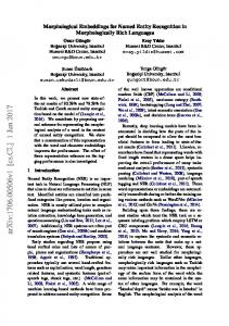
For a sequence CRF model, training and decoding can be solved efficiently by the Viterbi algorithm. 2.3. LSTM-CRF The neural network architecture is shown in Figure 1. The top strip-type stands for the observed variables, the oval represent deterministic functions of their outputs, and the bottom rectangle is the label. As describes in Section 2.2, the zi denotes the input of word representation at sentence level, and yi is the corresponding label. The process of producing word representation will be described in Section 2.4.3. The sequence of word representation is regarded as inputs to a bi-directional LSTM, and its output results from the right and left context (in Figure 1, Li is the left context and Ri is the right context for word i; Ci is the concatenation of Li and Ri) for each word in a sentence, as Section 2.1 presented. The output representation from bi-directional LSTM fed onto a CRF layer, the size of representation and its labels are equivalent. In order to consider the neighboring labels, instead of the softmax, we chose CRF as a decision function to yield final label sequence.
Entropy 2017, 19, 283
Patients
5 of 12
Taking
Acamprosate Concomitantly With
Antidepressants
Word represent
L1
L2
L3
L4
L5
L6 Bi-LSTM Encoding
R1
R2
R3
R4
R5
R6
C1
C2
C3
C4
C5
C6 CRF layer
o
o
B-DRUG
o
o
B-GROUP
Figure 1. The architecture of our model. Character level vector concatenated with word embedding as word representation. Firstly, put them into bi-directional long short-term memory (LSTM), then the outputs of the bi-directional LSTM network will be fed into the Conditional Random Fields (CRF) layer to decode the best label sequence. Then, add the dropout training into input and output layer during the bi-directional LSTM training.
2.4. Embedding and Network Training In this section, we provide the detail process of our neural network training. We apply the Theano library [22] to implement our system. We train our network architecture with the back-propagation algorithm to update the parameters for each training example with stochastic gradient descent (SGD). Our epoch size is set to 100. In each epoch, we divide all the training data into batches, then process one batch at a time. The batch size decides the number of sentences and our batch size is 100. In each batch, we firstly get the output scores from the bi-directional LSTM for all labels. Then we put the output scores into CRF model, and we can get the gradient of outputs and the state transition edges. From this, we can back propagate the error from output to input, which contains the backward propagation for bi-directional states of LSTM. Finally, we update the parameters including the Ai,j which represents the score of a transition from the tag i to tag j, and some other parameters such as U f , W f , b f from LSTM. 2.4.1. Parameters Initialization Word embedding: It is more efficient to use word embeddings than randomly initialized directly [23], we employed existing word embedding to initialize our lookup table. The word embedding are trained on entire English Wikipedia [24]. and produced by skip-n-gram [25] and Word2Vec [26], which account for word order. These embedding are fine-tuned during training.
Entropy 2017, 19, 283
6 of 12
Character embedding: character level evidence for a name is derived from orthographic feature. We apply character level features instead of hand-craft prefix and suffix construction features of words. It has been found that building character embedding is beneficial to learning representations in specific domains, and is always useful for morphologically rich languages and dealing with the out-of-vocabulary problem, such as part-of-speech tagging [25]. We collect all characters forming a character set which contains 26 upper and lower case letters (in our work, changing all letters to their lowercase), 10 numbers and 33 punctuation. The details are shown in Table 1. Table 1. The character set which contains 26 case letters, 10 numbers and 33 punctuations. Case Letters Numbers Punctuations
a|b|c|d|e|f|g|h|i|j|k|l|m|n|o|p|q|r|s|t|u|v|w|x|y|z 0|1|2|3|4|5|6|7|8|9 ˆ $|! %||&|*|-|=|_|+|(|)|||[|]|;|’|:|"|,|.|/||?|‘|’| |·||
26 10 33
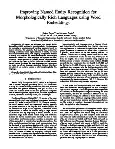
We initialized a character lookup table randomly with values ranging from low = −1.0 to high = 1.0 for the output of 50 dimensions embedding, which drew by a uniform distribution. Finally, our word representation is obtained by the architecture, which is shown in Figure 2. We construct character embedding with supervised training method using NER labels during the training process. Character level embedding for a word is given by direct and reverse order to the bi-directional LSTM with dimensions 25 respectively, and the result produces a vector with dimensions 50. Then we concatenated the result with its word embedding. Words out of the lookup table will be replaced as token “UNK“ and be mapped as UNK embedding, which is initialized by random. Refer to the paper [27], if a word is less than two letters we replace it with UNK embedding under a probability (p = 0.5).
a
c
i
d
la
lc
li
ld
ra
rc
ri
rd
lc rc Word embedding
Lookup table
w
Con-final embedding
Character embedding
acid
Figure 2. Feed character level embedding of the word “acid” into the bi-directional LSTM layer, then concatenate the outputs with the word embedding from lookup table as the final representation of the word “acid”.
Entropy 2017, 19, 283
7 of 12
2.4.2. Optimization Method We chose the mini-batch stochastic gradient descent, with a fixed learning rate of 0.01 and a gradient clipping of 5.0 [28], to optimize our parameters. Some similar methods have been applied to improve the performance of SGD, like Adadelta [29], Adam [30] and RMSProp [31]. Unfortunately, among the preliminary experiment [32], none of them could enhance the SGD. Dropout [33] can mitigate over-fitting. The paper [27] has proved that dropout can be beneficial to the NER task, which can avoid the over-fitting problem. So we apply dropout on the weight vectors directly to mask the final embedding layer before the combinational embedding feed into the bi-directional LSTM. We fix dropout rate at 0.5 as usual, and achieve good performance on our model. 2.4.3. Parameters Adjustment Our hyper-parameters showed in Table 2. In our experiment, referring to previous work [14,23,34], we set the state size of character for LSTM to 25 respectively for forward and backward, the dimension of character-based representation of words has been set at 50. The dimension of word embedding and word has been set at 100. The dimension of Con-Final Embedding has been set at 150. The dropout rate is 0.5 and initial learning rate is 0.01. Table 2. The parameters for our experiments. Hyper-Parameter initial state dropout rate initial learning rate gradient clipping word_dim forward_char_dim backward_char_dim char_dim con-final embedding
Values 0.0 0.5 0.01 5.0 100 25 25 50 150
2.5. IOBES Tagging Scheme Similar to the task of part-of-speech tagging, DNER also aims to assign a label to each word among a sentence. Due to there being some entity names containing more than one token in a sentence, typically, each token is encoded in IOB format (Inside, Outside, Begin), respectively if the token is inside (but not the first token within an entity name), or outside in entity name and the beginning of entity name. Take an example from Figure 1, from the part of a sentence “Patients| Taking| Acamprosate|Concomitantly|With| Antidepressants”, the corresponding label is “O|O| B–DRUG|O|O| B–GROUP”. 3. Experiments 3.1. Data Sets In our experiments, we primarily used the DDI2011 challenge corpus from the drug-drug interactions task (http://labda.inf.uc3m.es/DDIExtraction2011/). Refer to Task 9.1: Recognition and classification of drug names (http://www.cs.york.ac.uk/semeval-2013/task9/). For the DDI2011 challenge corpus, we use the NLP package Natural Language Toolkit (https://docs.python.org/ 2/library/xml.etree.elementtree.html) to parse all the XML format documents, then collect all the train dataset as the training data, and gather all the test dataset as the testing data. Table 3 shows the distribution of the documents, sentences and drugs in the train and test set from DDI2011. The train and test dataset contain 435 and 144 documents, 4267 and 1539 sentences, 11,260 and 3689 drugs respectively [35]. In this corpus, there is only one type with the entity name: drug, so each word in a
Entropy 2017, 19, 283
8 of 12
sentence just be labeled as “B/I-DRUG” or “O”. In our experiment, apart from replacing all digits with zero, we did not do any additional preprocessing on the challenge dataset. Table 3. Training and testing set in DDI2011. Set
Documents
Sentences
Drugs
Training Final Test Total
435 144 579
4267 1539 5806
11,260 3689 14,949
In order to further evaluate our model, we use the dataset from the Recognition and Classification of drug names task of SemEval-2013 (http://www.cs.york.ac.uk/semeval-2013/task9/). This task concerns the named entity extraction of mentions of pharmacological substances in text (https://www.cs.york.ac.uk/semeval-2013/task9/data/uploads/semeval_2013-task-9_1-evaluation metrics.pdf). Tables 4 and 5 show the numbers of the annotated entity in the DDI2013 training set and the testing set respectively. The corpus derives from two sources: DrugBank (https://www.drugbank.ca/) and MedLine (https://www.ncbi.nlm.nih.gov/pubmed/?term=meline). There are four general types of entities: Drug, Brand, Group, Drug_n [36]. Where Drug type is denoted as human medicines known as a generic name. The Brand type is characterized by a trade or brand name. Group type annotates groups of drugs. Finally, Drug_n type describes those substances like pesticides or toxins not available for human use. Table 4. Numbers of the annotated entities in DDI2013 training set. Type
DrugBank
MedLine
Total
Drug Brand Group Drug_n Total
9901 (63%) 1824 (12%) 3901 (25%) 130 (1%) 15,756
1745 (63%) 42 (1.5%) 324 (12%) 635 (23%) 2746
11,646 (63%) 1866 (10%) 4225 (23%) 765 (4%) 18,502
Table 5. Numbers of the annotated entities in DDI2013 testing set. Type
DrugBank
MedLine
Total
Drug Brand Group Drug_n Total
180 (59%) 53 (18%) 65 (21%) 6 (2%) 304
171 (44%) 6 (2%) 90 (24%) 115 (30%) 382
351 (51%) 59 (8%) 155 (23%) 121 (18%) 686
3.2. Evaluation Metrics In our experiment, we use precision recall, F1 to evaluate the performance of our system, and we use two of the four evaluation criteria provided by the DDI2013 challenge [36], the Type matching (a tagged drug name is correct only if there is some overlap between it and a gold drug name of the same class) and Strict matching (a tagged drug name is correct only if its boundary and class exactly match with a gold drug name). A detailed description of evaluation is in the document (https://www.cs.york.ac.uk/semeval2013/task9/data/uploads/semeval_2013-task-9_1-evaluationmetrics.pdf). Finally, we use evaluation scripts (https://www.cs.york.ac.uk/semeval-2013/task9/index. php%3Fid=evaluation.html) provided by the shared task organizers to evaluate our system.
Entropy 2017, 19, 283
9 of 12
3.3. Results Table 6 displays the results of the experiment, which was performed on the DDI2011 corpus. We can achieve the precision of 93.26%, recall of 91.11% and F1 of 92.04%. Comparing our result with previous best results [37], which were obtained by building a man-made dictionary and using CRF method we find that our precision is lower than the best performance by 1.5%. However, our recall is higher than the best performance by 0.6%. However, when their system just uses CRF method without the dictionary assistant, the performance of our system outperforms their evaluation values. Table 6. Results of experiment in DDI2011. System
Precision
Recall
F1
Our System Best without Dic Best with Dic
93.26% (−1.5%) 92.15% 94.75%
91.11% (+0.6%) 89.73% 90.44%
92.04% (−0.5%) 90.92% 92.54%
Table 7 shows all types of the entities and their detailed evaluation. We can observe that our method is efficient in correctly classifying the Drug, Brand and Group types, where it achieves an F1 of over 80% correspondingly. However, our method has a few difficulties in correctly classifying named entities of the Drug_n type, the F1 of 62.83% was achieved. A previous work [38] showed that the Drug_n entity type was demonstrated to be a very difficult type to be classified correctly. According to our analysis, the low percentage of this type in the training dataset (