LSTM Shift-Reduce CCG Parsing - Association for Computational ...
Recommend Documents
E-mail: [email protected]. ââ School .... in this figure is that the dependency links always emanate from the last IG of a word, because ... treebank.html.
1985) or func- tional unification grammars (cf. Karttunnen &: Kay 1985). ... of our parser for German, which is able to han- dle the difficulties arising from word ...
un dolce di frutta ha ordinato il maestro a cake with fruits has ordered the teacher and in general all the five permutations of the "basic". (i.e. more likely) SVO ...
tion choices, and parsing model design (Levy and. Manning, 2003 ... with previous work, we exhaustively evaluate this grammar and two ... inna and her sisters since they can be inflected, the ATB ... common in the ATBâwhere (1) will follow a verb l
subtrees approachâ, Collins & Duffy, 2002). ... ternative approaches to statistical parsing (Collins,. 1997 ...... Slav Petrov, Leon Barrett, Romain Thibaux, and Dan.
Aug 23, 2014 - For many NLP-applications, including machine translation, ... In formal terms that we need for the outline of the transduction below, a SSyntS is ...
May 17, 2015 - gold standard and show that our model significantly outperforms the baseline model ... We conclude that despite the limited settings, there are no- ... I would also like to thank Bharat Ram Ambati who was very helpful in giving ..... m
lucky/ADJ. Index: 3228~3233. Feature. Retrieval. Parse Tree. Build lattice, inference etc. Figure 1: Flow chart of .... Trie stores strings over a fixed alphabet, in our.
a given parsing algorithm Alg is denoted 2:Alg, the .... such that N ~ 2_+ 5v ⢠P(3"), 3" E I U A, 0 < i < j, (p,q)
Ryan McDonald, Kevin Lerman, and Fernando Pereira. 2006. Multilingual dependency analysis with a two- stage discriminative parser. In Proc. CoNLL, pages.
Jun 17, 2016 - tron algorithm (Collins, 2002) predictions by those of an FFNN at the ..... David Weiss, Chris Alberti, Michael Collins, and Slav. Petrov. 2015.
structure of a sentence is required; hence a lot of research is being done on ... words length, LDA parser determines the correct full-parse of the sentence with ...
Proceedings of the Workshop on Machine Translation and Parsing in Indian Languages ... the training data contained 12041 sentences (268,093 words) and the ... provide details on the parsing and learning approaches used in the system, ...
Mar 23, 2016 - Adobe Research. Abstract. By taking .... LSTM layers to improve the network training with many layers. these previous .... and Upper/Lower Legs, resulting in six person part classes and one background class. 1, 716 images ...
tions, while learning significantly more compact ...... the same number of inference calls, and in prac- .... Proceeding
Aug 23, 2014 - use the feature templates of Bohnet (2010) as our base feature templates, which produces ... [wp]hâ1, [wp]h, [wp]c, [wp]c+1, d(h, d, c). [wp]h ...
language without considering syntax. We describe ... therefore a complete syntactic parsing of the sentence. ..... ellipses and the interruptions, Our parser is thus.
machine learning techniques learn the rules ... selection of the most interesting learned rules; c) incorporation .... is a machine learning library developed in C++.
2 Method. This section starts with a description of the three tasks that we have ... conventional probabilistic context-free produc- ... grammar's set of nonterminals. ..... Six members of the project have performed this task. The results of the six
human brains acquire and exploit language, we are driven to ... the project is a synthesis of cognitive linguistics .... Special thanks for this presentation go to John.
Keywords: Nested graphs, Universal Networking Language, Semantic Graph ...
In this paper, we describe the identification of semantic sub-graphs from Tamil,.
Jun 1, 2018 - Laura Banarescu, Claire Bonial, Shu Cai, Madalina. Georgescu, Kira Griffitt, Ulf .... The penn chinese treebank: Phrase structure annotation of a ...
resentation towards a single interpretation. Graded constraints are used as means to express well- .... constructions from being handled properly, because.
Dahl, Deborah A. 1985 The Structure and Function of one-anaphora in. English. Indiana University Linguistics Club, Bloomington, Indiana. Dahl, Deborah A.
LSTM Shift-Reduce CCG Parsing - Association for Computational ...
Lewis et al., 2016; Vaswani et al., 2016; Xu et al.,. 2016), and ... ments over non-recurrent models (Lewis and Steed- man, 2014b). ..... Joshua Goodman. 1996.
LSTM Shift-Reduce CCG Parsing
Wenduan Xu Computer Laboratory University of Cambridge [email protected]
Abstract We describe a neural shift-reduce parsing model for CCG, factored into four unidirectional LSTMs and one bidirectional LSTM. This factorization allows the linearization of the complete parsing history, and results in a highly accurate greedy parser that outperforms all previous beam-search shift-reduce parsers for CCG. By further deriving a globally optimized model using a task-based loss, we improve over the state of the art by up to 2.67% labeled F1.
1
Introduction
Combinatory Categorial Grammar (CCG; Steedman, 2000) parsing is challenging due to its so-called “spurious” ambiguity that permits a large number of non-standard derivations (Vijay-Shanker and Weir, 1993; Kuhlmann and Satta, 2014). To address this, the de facto models resort to chart-based CKY (Hockenmaier, 2003; Clark and Curran, 2007), despite CCG being naturally compatible with shiftreduce parsing (Ades and Steedman, 1982). More recently, Zhang and Clark (2011) introduced the first shift-reduce model for CCG, which also showed substantial improvements over the long-established state of the art (Clark and Curran, 2007). The success of the shift-reduce model (Zhang and Clark, 2011) can be tied to two main contributing factors. First, without any feature locality restrictions, it is able to use a much richer feature set; while intensive feature engineering is inevitable, it has nevertheless delivered an effective and conceptually simpler alternative for both parameter estimation and inference. Second, it couples beam search
with global optimization (Collins, 2002; Collins and Roark, 2004; Zhang and Clark, 2008), which makes it less prone to search errors than fully greedy models (Huang et al., 2012). In this paper, we present a neural architecture for shift-reduce CCG parsing based on long short-term memories (LSTMs; Hochreiter and Schmidhuber, 1997). Our model is inspired by Dyer et al. (2015), in which we explicitly linearize the complete history of parser states in an incremental fashion by requiring no feature engineering (Zhang and Clark, 2011; Xu et al., 2014), and no atomic feature sets (Chen and Manning, 2014). However, a key difference is that we achieve this linearization without relying on any additional control operations or compositional tree structures (Socher et al., 2010; Socher et al., 2011; Socher et al., 2013), both of which are vital in the architecture of Dyer et al. (2015). Crucially, unlike the sequence-to-sequence transduction model of Vinyals et al. (2015), which primarily conditions on the input words, our model is sensitive to all aspects of the parsing history, including arbitrary positions in the input. As another contribution, we present a global LSTM parsing model by adapting an expected Fmeasure loss (Xu et al., 2016). As well as naturally incorporating beam search during training, this loss optimizes the model towards the final evaluation metric (Goodman, 1996; Smith and Eisner, 2006; Auli and Lopez, 2011b), allowing it to learn shiftreduce action sequences that lead to parses with high expected F-scores. We further show the globally optimized model can be leveraged with greedy inference, resulting in a deterministic parser as accurate
Dexter
likes
experiments
NP
(S \NP )/NP
NP
>T
S /(S \NP ) >B
S /NP S
>
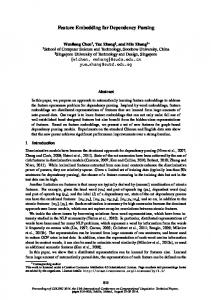
Figure 1: A CCG derivation, in which each point corresponds to the result of a shift-reduce action. In this example, composition (B) and application (>) are re actions, and type-raising (T) is a un action.
as its beam-search counterpart. On standard CCGBank tests, we clearly outperform all previous shift-reduce CCG parsers; and by combining the parser with an attention-based LSTM supertagger (§4), we obtain further significant improvements (§5).
2
Shift-Reduce CCG Parsing
is strongly lexicalized by definition. A CCG grammar extracted from CCGBank (Hockenmaier and Steedman, 2007) contains over 400 lexical types and over 1,500 non-terminals (Clark and Curran, 2007), which is an order of magnitude more than those of a typical CFG parser. This lexicalized nature raises another unique challenge for parsing— any parsing model for CCG needs to perform lexical disambiguation. This is true even in the approach of Fowler and Penn (2010), in which a contextfree cover grammar extracted from CCGBank is used to parse CCG. Indeed, as noted by Auli and Lopez (2011a), the search problem for CCG parsing is equivalent to finding an optimal derivation in the weighted intersection of a regular language (generated by the supertagger) and a mildly contextsensitive language (generated by the parser), which can quickly become expensive. The shift-reduce paradigm (Aho and Ullman, 1972; Yamada and Matsumoto, 2003; Nivre and Scholz, 2004) applied to CCG (Zhang and Clark, 2011) presents a more elegant solution to this problem by allowing the parser to conduct lexical assignment “incrementally” as a complete parse is being built by the decoder. This is not possible with a chart-based parser, in which complete derivations must be built first. Therefore, a shift-reduce parser is able to consider a much larger set of categories per word for a given input, achieving higher lexiCCG
cal assignment accuracy than the C & C parser (Clark and Curran, 2007), even with the same supertagging model (Zhang and Clark, 2011; Xu et al., 2014). In our parser, we follow this strategy and adopt the Zhang and Clark (2011) style shift-reduce transition system, which assumes a set of lexical categories has been assigned to each word using a supertagger (Bangalore and Joshi, 1999; Clark and Curran, 2004). Parsing then proceeds by applying a sequence of actions to transform the input maintained on a queue, into partially constructed derivations, kept on a stack, until the queue and available actions on the stack are both exhausted. At each time step, the parser can choose to shift (sh) one of the lexical categories of the front word onto the stack, and remove that word from the queue; reduce (re) the top two subtrees on the stack using a CCG rule, replacing them with the resulting category; or take a unary (un) action to apply a CCG type-raising or type-changing rule to the stack-top element. For example, the deterministic sequence of shift-reduce actions that builds the derivation in Fig.1 is: sh ⇒ NP , un ⇒ S /(S \NP ), sh ⇒ (S \NP )/NP , re ⇒ S /NP , sh ⇒ NP and re ⇒ S , where we use ⇒ to indicate the CCG category produced by an action.1
3
LSTM Shift-Reduce Parsing
3.1
LSTM
Recurrent neural networks (RNNs; e.g., see Elman, 1990) are factored into an input layer xt and a hidden state (layer) ht with recurrent connections, and they can be represented by the following recurrence: ht = Φθ (xt , ht−1 ),
(1)
where xt is the current input, ht−1 is the previous hidden state and Φ is a set of affine transformations parametrized by θ. Here, we use a variant of RNN referred to as LSTMs, which augment Eq. 1 with a cell state, ct , s.t. ht , ct = Φθ (xt , ht−1 , ct−1 ).
(2)
Compared with conventional RNNs, this extra facility gives LSTMs more persistent memories over 1
Our parser models normal-form derivations (Eisner, 1996) in CCGBank. However, unlike Zhang and Clark (2011), derivations are not restricted to be normal-form during inference.
longer time delays and makes them less susceptible to the vanishing gradient problem (Bengio et al., 1994). Hence, they are better at modeling temporal events that are arbitrarily far in a sequence. Several extensions to the vanilla LSTM have been proposed over time, each with a modified instantiation of Φθ that exerts refined control over e.g., whether the cell state could be reset (Gers et al., 2000) or whether extra connections are added to the cell state (Gers and Schmidhuber, 2000). Our instantiation is as follows for all LSTMs: it = σ(Wix xt + Wih ht−1 + Wic ct−1 + bi ) ft = σ(Wf x xt + Wf h ht−1 + Wf c ct−1 + bf ) ct = ft ct−1 + it tanh(Wcx xt + Wch ht−1 + bc ) ot = σ(Wox xt + Woh ht−1 + Woc ct + bo ) ht = ot tanh(ct ), where σ is the sigmoid activation and is the element-wise product. In addition to unidirectional LSTMs that model an input sequence x0 , x1 , . . . , xn−1 in a strict leftto-right order, we also use bidirectional LSTMs (BLSTMs; Graves and Schmidhuber, 2005), which read the input from both directions with two independent LSTMs. At each step, the forward hidden state ht is computed using Eq. 2 for t = (0, 1, . . . , n − 1); and the backward hidden state hˆt is computed similarly but from the reverse direction for t = (n − 1, n − 2, . . . , 0). Together, the two hidden states at each step t capture both past and future contexts, and the representation for each xt is ˆ t ]. obtained as the concatenation [ht ; h 3.2
Embeddings
The neural network model employed by Chen and Manning (2014), and followed by a number of other parsers (Weiss et al., 2015; Zhou et al., 2015; Ambati et al., 2016; Andor et al., 2016; Xu et al., 2016) allows higher-order feature conjunctions to be automatically discovered from a set of dense feature embeddings. However, a set of atomic feature templates, which are only sensitive to contexts from the top few elements on the stack and queue are still needed to dictate the choice of these embeddings. Instead, we dispense with such templates and seek
t : (j, δ|s1 |s0 , β, ∆) t + 1 : (j, δ|x, β, ∆ ∪ hxi))
(re; s1 s0 → x)
t : (j, δ|s0 , β, ∆) t + 1 : (j, δ|x, β, ∆)
(un; s0 → x)
Figure 2: The shift-reduce deduction system. For the sh deduction, xwj denotes an available lexical category for wj ; for re, hxi denotes the set of dependencies on x.
to design a model that is sensitive to both local and non-local contexts, on both the stack and queue. Consequently, embeddings represent atomic input units that are added to our parser and are preserved throughout parsing. In total we use four types of embeddings, namely, word, CCG category, POS and action, where each has an associated look-up table that maps a string of that type to its embedding. The look-up table for words is Lw ∈ Rk×|w| , where k is the embedding dimension and |w| is the size of the vocabulary. Similarly, we have look-up tables for CCG categories, Lc ∈ Rl×|c| , for the three types of actions, La ∈ Rm×3 , and for POS tags, Lp ∈ Rn×|p| . 3.3
Model
Parser. Fig. 2 shows the deduction system of our parser.2 We denote each parse item as (j, δ, β, ∆), where j is the positional index of the word at the front of the queue, δ is the stack (with its top element s0 to the right), and β is the queue (with its top element wj to the left) and ∆ is the set of CCG dependencies realized for the input consumed so far. Each item is also associated with a step indicator t, signifying the number of actions applied to it and the goal is reached in 2n − 1 + µ steps, where µ is the total number of un actions. We also define each action in our parser as a 4-tuple (τt , ct , wct , pwct ), where τt ∈ {sh, re, un} for t ≥ 1, ct is the resulting category of τt , and wct is the head word attached to 2
We assume greedy inference unless otherwise stated.
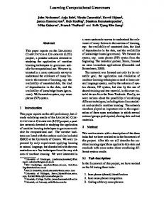
where B is a parameter matrix of the model, r is a bias vector and f is a ReLU non-linearity (Nair and Hinton, 2010). Then we apply another affine transformation (with A as the weights and s as the bias) to bt : at = f (Abt + s), Figure 3: An example representation for a parse item at time step t, with the 4 unidirectional LSTMs (left) and the bidirectional LSTM (right). The shaded cells on the left represent δt = [hUt ; hVt ; hXt ; hYt ] (Eq. 3), and the shaded cells on the right ˆW represent wj = [hW j ; hj ].
LSTM model. LSTMs are designed to handle time-series data, in a purely sequential fashion, and we try to exploit this fact by completely linearizing all aspects of the parsing history. Concretely, we factor the model as five LSTMs, comprising four unidirectional ones, denoted as U, V, X and Y, and an additional BLSTM, denoted as W (Fig. 3). Before parsing each sentence, we feed W with the complete input (padded with a special embedding ⊥ as the end ˆW of sentence token); and we use wj = [hW j ; hj ] to represent wj in subsequent steps.4 We also add ⊥ to the other 4 unidirectional LSTMs as initialization. Given this factorization, the stack representation for a parse item (j, δ, β, ∆) at step t, for t ≥ 1, is obtained as (3)
and together with wj , [δt ; wj ] gives a representation for the parse item. For the axiom item, we represent Y V X it as [δ0 ; w0 ], where δ0 = [hU ⊥ ; h⊥ ; h⊥ ; h⊥ ]. Each time the parser applies an action (τt , ct , wct , pwct ), we update the model by adding the embedding of τt , denoted as La (τt ), onto U, and adding the other three embeddings of the action 4-tuple, that is, Lc (ct ), Lw (wct ) and Lp (pwct ), onto V, X and Y respectively. To predict the next action, we first derive an action hidden layer bt , by passing the parse item representation [δt ; wj ] through an affine transformation, s.t. bt = f (B[δt ; wj ] + r), 3
(4)
In case of multiple heads, we always choose the first one. Word and POS embeddings are concatenated at each input ˆW position j, for 0 ≤ j < n; and wn = [hW ⊥ ; h⊥ ]. 4
exp{ait } , k τ k ∈T (δt ,βt ) exp{at }
p(τti |bt ) = P
t
where T (δt , βt ) is the set of feasible actions for the current parse item, and τti ∈ T (δt , βt ).
ct with pwct being its POS tag.3
V X Y δt = [hU t ; ht ; ht ; ht ],
and obtain the probability of the ith action in at as
3.4
Derivations and Dependency Structures
Our model naturally linearizes CCG derivations “incrementally” following their post-order traversals. As such, the four unidirectional LSTMs always have the same number of steps; and at each step, the concatenation of their hidden states (Eq. 3) represents a point in a CCG derivation (i.e., an action 4-tuple). Due to the large amount of flexibility in how dependencies are realized in CCG (Hockenmaier, 2003; Clark and Curran, 2007), and in line with most existing CCG parsing models, including dependency models, we have chosen to model CCG derivations, rather than dependency structures.5 We also hypothesize that tree structures are not necessary for the current model, since they are already implicit in the linearized derivations; similarly, we have found the action embeddings to be nonessential (§5.2). 3.5
Training
As a baseline, we first train a greedy model, in which we maximize the log-likelihood of each target action in the training data. More specifically, let (τ1g , . . . , τTgn ) be the gold-standard action sequence for a training sentence n, a cross-entropy criterion is used to obtain the error gradients, and for each sentence, training involves minimizing L(θ) = − log
Tn Y t=1
p(τtg |bt ) = −
Tn X
log p(τtg |bt ),
t=1
where θ is the set of all parameters in the model. 5
Most CCG dependency models (e.g., see Clark and Curran (2007) and Xu et al. (2014)) model CCG derivations with dependency features.
As other greedy models (e.g., see Chen and Manning (2014) and Dyer et al. (2015)), our greedy model is locally optimized, and suffers from the label bias problem (Andor et al., 2016). A partial solution to this is to use beam search at test time, thereby recovering higher scoring action sequences that would otherwise be unreachable with fully greedy inference. In practice, this has limited effect (Table 2), and a number of more principled solutions have been recently proposed to derive globally optimized models during training (Watanabe and Sumita, 2015; Weiss et al., 2015; Zhou et al., 2015; Andor et al., 2016). Here, we extend our greedy model into a global one by adapting the expected F-measure loss of Xu et al. (2016). To our best knowledge, this is the first attempt to train a globally optimized LSTM shift-reduce parser. Let θ = {U, V, X, Y, W, B, A} be the weights of the baseline greedy model,6 we initialize the weights of the global model, which has the same architecture as the baseline, to θ, and we reoptimize θ in multiple training epochs as follows: 1. Pick a sentence xn from the training set, decode it with beam search, and generate a k-best list of output parses with the current θ, denoted as Λ(xn ).7 2. For each parse yi in Λ(xn ), compute its sentence-level F1 using the set of dependencies in the ∆ field of its parse item. In addition, let |yi | be the total number of actions that derived yi and sθ (yij ) be the softmax action score of the j th action, given by the LSTM model. Compute the log-linear score of its action sequence P|yi | as ρ(yi ) = j=1 log sθ (yij ). 3. Compute the negative expected F1 objective (defined below) for xn and minimize it using stochastic gradient descent (maximizing expected F1). Repeat these three steps for the remaining sentences. 6 We use boldface letters to designate the weights of the corresponding LSTMs, and omit bias terms for brevity. 7 As in Xu et al. (2016), we did not preset k, and found k = 11.06 on average with a beam size of 8 that we used for this training.
More formally, the loss J(θ), is defined as J(θ) = −XF1(θ) X p(yi |θ)F1(∆yi , ∆G =− xn ), yi ∈Λ(xn )
where F1(∆yi , ∆G xn ) is the sentence level F1 of the parse derived by yi , with respect to the gold-standard dependency structure ∆G xn of xn ; p(yi |θ) is the normalized probability score of the action sequence yi , computed as exp{γρ(yi )} , y∈Λ(xn ) exp{γρ(y)}
p(yi |θ) = P
where γ is a parameter that sharpens or flattens the distribution (Tromble et al., 2008).8 Different from the maximum-likelihood objective, XF1 optimizes the model on a sequence level and towards the final evaluation metric, by taking into account all action sequences in Λ(xn ).
4
Attention-Based LSTM Supertagging
In addition to the size of the label space, supertagging is difficult because CCG categories can encode long-range dependencies and tagging decisions frequently depend on non-local contexts. For example, in He went to the zoo with a cat, a possible category for with, (S \NP )\(S \NP )/NP , depends on the word went further back in the sentence. Recently a number of RNN models have been proposed for CCG supertagging (Xu et al., 2015; Lewis et al., 2016; Vaswani et al., 2016; Xu et al., 2016), and such models show dramatic improvements over non-recurrent models (Lewis and Steedman, 2014b). Although the underlying models differ in their exact architectures, all of them make each tagging decision using only the hidden states at the current input position, and this imposes a potential bottleneck in the model. To mitigate this, we generalize the attention mechanisms of Bahdanau et al. (2015) and Luong et al. (2015), and adapt them to supertagging, by allowing the model to explicitly use hidden states from more than one input positions for tagging each word. Similar to Bahdanau et al. (2015) and Luong et al. (2015), a key feature in 8
We found γ = 1 to be a good choice during development.
our model is a soft alignment vector that weights the relative importance of the considered hidden states. For an input sentence w0 , w1 , . . . , wn−1 , we conˆ t ] (§3.1) to be the representasider wt = [ht ; h th tion of the t word (0 ≤ t < n, wt ∈ R2d×1 ), given by a BLSTM with a hidden state size d for both its forward and backward layers.9 Let k be a context window size hyperparameter, we define Ht ∈ R2d×(k−1) as Ht = [wt−bk/2c , . . . , wt−1 , wt+1 , . . . , wt+bk/2c ], which contains representations for all words in the size k window except wt . At each position t, the attention model derives a context vector ct ∈ R2d×1 (defined below) from Ht , which is used in conjunction with wt to produce an attentional hidden layer: xt = f (M[ct ; wt ] + m),
(5)
where f is a ReLU non-linearity, M ∈ Rg×4d is a learned weight matrix, m is a bias term, and g is the size of xt . Then xt is used to produce another hidden layer (with N as the weights and n as the bias): zt = Nxt + n, and the predictive distribution over categories is obtained by feeding zt through a softmax activation. In order to derive the context vector ct , we first compute bt ∈ R(k−1)×1 from Ht and wt using α ∈ R1×4d , s.t. the ith entry in bt is bit = α[wT [i] ; wt ], for i ∈ [0, k−1), T = [t−bk/2c, . . . , t−1, t+1, . . . , t+ bk/2c]; and ct is derived as follows: at = softmax(bt ), ct = Ht at , where at is the alignment vector. We also experiment with two types of attention reminiscent of the global and local models in Luong et al. (2015), where the first attends over all input words (k = n) and the second over a local window. It is worth noting that two other works have concurrently tackled supertagging with BLSTM models. In Vaswani et al. (2016), a language model 9
Unlike in the parsing model, POS tags are excluded.
layer is added on top of a BLSTM, which allows embeddings of previously predicted tags to propagate through and influence the pending tagging decision. However, the language model layer is only effective when both scheduled sampling for training (Bengio et al., 2015) and beam search for inference are used. We show our attention-based models can match their performance, with only standard training and greedy decoding. Additionally, Lewis et al. (2016) presented a BLSTM model with two layers of stacking in each direction; and as an internal baseline, we show a non-stacking BLSTM without attention can achieve the same accuracy.
5
Experiments
Dataset and baselines. We conducted all experiments on CCGBank (Hockenmaier and Steedman, 2007) with the standard splits.10 We assigned POS tags with the C & C POS tagger, and used 10-fold jackknifing for both POS tagging and supertagging. All parsers were evaluated using F1 over labeled CCG dependencies. For supertagging, the baseline models are the RNN model of Xu et al. (2015), the bidirectional RNN (BRNN) model of Xu et al. (2016), and the BLSTM supertagging models in Vaswani et al. (2016) and Lewis et al. (2016). For parsing experiments, we compared with the global beam-search shift-reduce parsers of Zhang and Clark (2011) and Xu et al. (2014). One neural shift-reduce CCG parser baseline is Ambati et al. (2016), which is a beam-search shift-reduce parser based on Chen and Manning (2014) and Weiss et al. (2015); and the others are the RNN shift-reduce models in Xu et al. (2016). Additionally, the chart-based C & C parser was included by default. Model and training parameters.11 All our LSTM models are non-stacking with a single layer.12 For the supertagging models, the LSTM 10
Training: Sections 02-21 (39,604 sentences). Development: Section 00 (1,913 sentences). Test: Section 23 (2,407 sentences). 11 We implemented all models using the CNN toolkit: https://github.com/clab/cnn. 12 The BLSTMs have a single layer in each direction. We experimented with 2 layers in all models during development and found negligible improvements.
Model C&C Xu et al. (2015) Xu et al. (2016) Lewis et al. (2016) Vaswani et al. (2016) Vaswani et al. (2016) +LM +beam BLSTM BLSTM-local BLSTM-global
Dev 91.50 93.07 93.49 94.1 94.08 94.24 94.11 94.31 94.22
Test 92.02 93.00 93.52 94.3 94.50 94.29 94.46 94.42
Table 1: 1-best supertagging results on both the dev and test sets. BLSTM is the baseline model without attention; BLSTMlocal and -global are the two attention-based models.
hidden state size is 256, and the size of the attentional hidden layer (xt , Eq. 5) is 200. All parsing model LSTMs have a hidden state size of 128, and the size of the action hidden layer (bt , Eq. 4) is 80. Pretrained word embeddings for all models are 100-dimensional (Turian et al., 2010), and all other embeddings are 50-dimensional. We also pretrained CCG lexical category and POS embeddings on the concatenation of the training data and a Wikipedia dump parsed with C & C.13 p All other parameters were uniformly initialized in ± 6/(r + c), where r and c are the number of rows and columns of a matrix (Glorot and Bengio, 2010). For training, we used plain non-minibatched stochastic gradient descent with an initial learning rate η0 = 0.1 and we kept iterating in epochs until accuracy no longer increases on the dev set. For all models, a learning rate schedule ηe = η0 /(1 + λe) with λ = 0.08 was used for e ≥ 11. Gradients were clipped whenever their norm exceeds 5. Dropout training as suggested by Zaremba et al. (2014), with a dropout rate of 0.3, and an `2 penalty of 1 × 10⁻⁵ , were applied to all models. 5.1
Supertagging Results
Table 1 summarizes 1-best supertagging results. Our baseline BLSTM model without attention achieves the same level of accuracy as Lewis et al. (2016) and the baseline BLSTM model of Vaswani et al. (2016). Compared with the latter, our hidden state size is 50% smaller (256 vs. 512). For training and testing the local attention model (BLSTM-local), we used an attention window size 13
We used the gensim word2vec toolkit: radimrehurek.com/gensim/.
Table 2: Tuning beam size and supertagger β on the dev set.
Model LSTM-w LSTM-w+c LSTM-w+c+a LSTM-w+c+a+p
LP 90.13 89.37 89.31 89.43
LR 76.99 83.25 83.39 83.86
LF 83.05 86.20 86.25 86.56
CAT 94.24 94.34 94.38 94.47
Table 3: F1 on dev for all the greedy models.
of 5 (tuned on the dev set), and it gives an improvement of 0.94% over the BRNN supertagger (Xu et al., 2016), achieving an accuracy on par with the beam-search (size 12) model of Vaswani et al. (2016) that is enhanced with a language model. Despite being able to consider wider contexts than the local model, the global attention model (BLSTMglobal) did not show further gains, hence we used BLSTM-local for all parsing experiments below. 5.2
Parsing Results
All parsers we consider use a supertagger probability cutoff β to prune categories less likely than β times the probability of the best category in a distribution: for the C & C parser, it uses an adaptive strategy to backoff to smaller β values if no spanning analysis is found given an initial β setting; for all the shift-reduce parsers, fixed β values are used without backing off. Since β determines the derivation space of a parser, it has a large impact on the final parsing accuracy. For the maximum-likelihood greedy model, we found using a small β value (bigger ambiguity) for training significantly improved accuracy, and we chose β = 1 × 10⁻⁵ (5.22 categories per word with jackknifing) via development experiments. This reinforces the findings in a number of other CCG parsers (Clark and Curran, 2007; Auli and Lopez, 2011a; Lewis and Steedman, 2014a): even though a smaller β increases ambiguity, it leads to more accurate models at test time. On the other hand, we found using larger β values at test time led to significantly better results (Table 2). And this differs from the beam-search models that use the same β value for both training and testing (Zhang and Clark, 2011; Xu et al., 2014).
F1 (labeled) on dev set
F1 (labeled) on dev set
87 86 85 84 83 82 81 80 79 78
LSTM-w LSTM-wc LSTM-wca LSTM-wcap 0
5
10 15 20 Training epochs
25
30
87.5 87.4 87.3 87.2 87.1 87 86.9 86.8 86.7 86.6
LSTM-XF1 (beam = 8) 0
(a) Dev F1 of the greedy models
5
10 15 Training epochs
20
(b) Dev F1 of the XF1 model
Figure 4: Learning curves with dev F-scores for all models.
Model C & C (normal-form) C & C (dependency hybrid) Zhang and Clark (2011) Xu et al. (2014) Ambati et al. (2016) Xu et al. (2016)-greedy Xu et al. (2016)-XF1 LSTM-greedy LSTM-XF1 LSTM-XF1
Table 4: Parsing results on the dev (Section 00) and test (Section 23) sets with 100% coverage, with all LSTM models using the BLSTM-local supertagging model. All experiments using auto POS. CAT (lexical category assignment accuracy). LSTM-greedy is the full greedy parser.
The greedy model. Table 3 shows the dev set results for all greedy models, where the four types of embeddings, that is, word (w), CCG category (c), action (a) and POS (p), are gradually introduced. The full model LSTM-w+c+a+p surpasses all previous shift-reduce models (Table 4), achieving a dev set accuracy of 86.56%. Category embeddings (LSTM-w+c) yielded a large gain over using word embeddings alone (LSTM-w); action embeddings (LSTM-w+c+a) provided little improvement, but further adding POS embeddings (LSTMw+c+a+p) gave noticeable recall (+0.61%) and F1 improvements (+0.36%) over LSTM-w+c. Fig. 4a shows the learning curves, where all models converged in under 30 epochs. The XF1 model. Table 4 also shows the results for the XF1 models (LSTM-XF1), which use all four types of embeddings. We used a beam size of 8, and
Model LSTM-BRNN LSTM-BLSTM LSTM-greedy
Dev 85.86 86.26 86.56
Test 86.37 86.64 86.83
Table 5: Effect of different supertaggers on the full greedy parser. LSTM-greedy is the same parser as in Table 4, which uses the BLSTM-local supertagger.
a β value of 0.06 for both training and testing (tuned on the dev set); and training took 12 epochs to converge (Fig. 4b), with an F1 of 87.45% on the dev set. Decoding the XF1 model with greedy inference only slightly decreased recall and F1, and this resulted in a highly accurate deterministic parser. On the test set, our XF1 greedy model gives 2.67% F1 improvement over the greedy model in Xu et al. (2016); and the beam-search XF1 model achieves an F1 improvement of 1.34% compared with the XF1 model of Xu et al. (2016).
Model Xu et al. (2015) Lewis et al. (2016) Lewis et al. (2016)? Vaswani et al. (2016)∗ Lee et al. (2016) LSTM-XF1 (beam = 1) LSTM-XF1 (beam = 8)
LP 87.68 87.7 88.6 89.85 89.81
LR 86.41 86.7 87.5 85.51 85.81
LF 87.04 87.2 88.1 88.32 88.7 87.62 87.76
Table 6: Comparison of our XF1 models with chart-based parsers on the test set. ? denotes a tri-trained model and ∗ indicates a different POS tagger.
Effect of the supertagger. To isolate the parsing model from the supertagging model, we first experimented with the BRNN supertagging model as in Xu et al. (2016) for both training and testing the full greedy LSTM parser. Using this supertagger, we still achieved the highest F1 (85.86%) on the dev set (LSTM-BRNN, Table 5) in comparison with all previous shift-reduce models; and an improvement of 1.42% F1 over the greedy model of Xu et al. (2016) was obtained on the test set (Table 4). We then experimented with using the baseline BLSTM supertagging model for parsing (LSTM-BLSTM), and observed the attention-based setup (LSTM-greedy) outperformed it, despite the attention-based supertagger (BLSTM-local) did not give better multi-tagging accuracy. We owe this to the fact that large β cutoff values—resulting in almost deterministic supertagging decisions on average—are required by the parser during inference; for instance, BLSTM-local has an average ambiguity of 1.09 on the dev set with β = 0.06.14 Comparison with chart-based models. For completeness and to put our results in perspective, we compare our XF1 models with other CCG parsers in the literature (Table 6): Xu et al. (2015) is the log-linear C & C dependency hybrid model with an RNN supertagger front-end; Lewis et al. (2016) is an LSTM supertagger-factored parser using the A∗ CCG parsing algorithm of Lewis and Steedman (2014a); Vaswani et al. (2016) combine a BLSTM supertagger with a new version of the C & C parser (Clark et al., 2015) that uses a max-violation perceptron, which significantly improves over the 14
All β cutoffs were tuned on the dev set; for BRNN, we found the same β settings as in Xu et al. (2016) to be optimal; for BLSTM, β = 4 × 10⁻⁵ for training (with an ambiguity of 5.27) and β = 0.02 for testing (with an ambiguity of 1.17).
original C & C models; and finally, a global recursive neural network model with A∗ decoding (Lee et al., 2016). We note that all these alternative models— with the exception of Xu et al. (2015) and Lewis et al. (2016)—use structured training that accounts for violations of the gold-standard, and we conjecture further improvements for our model are possible by incorporating such mechanisms.15
6
Conclusion
We have presented an LSTM parsing model for CCG, with a factorization allowing the linearization of the complete parsing history. We have shown that this simple model is highly effective, with results outperforming all previous shift-reduce CCG parsers. We have also shown global optimization benefits an LSTM shift-reduce model; and contrary to previous findings with the averaged perceptron (Zhang and Clark, 2008), we empirically demonstrated beamsearch inference is not necessary for our globally optimized model. For future work, a natural direction is to explore integrated supertagging and parsing in a single neural model (Zhang and Weiss, 2016).
Acknowledgment I acknowledge the support from the Carnegie Trust for the Universities of Scotland through a Carnegie Scholarship.
References Anthony Ades and Mark Steedman. 1982. On the order of words. In Linguistics and philosophy. Springer. Alfred Aho and Jeffrey Ullman. 1972. The theory of parsing, translation, and compiling. Prentice-Hall. Bharat Ram Ambati, Tejaswini Deoskar, and Mark Steedman. 2016. Shift-reduce CCG parsing using neural network models. In Proc. of NAACL (Volume 2). Daniel Andor, Chris Alberti, David Weiss, Aliaksei Severyn, Alessandro Presta, Kuzman Ganchev, Slav Petrov, and Michael Collins. 2016. Globally normalized transition-based neural networks. In Proc. of ACL. Michael Auli and Adam Lopez. 2011a. A comparison of loopy belief propagation and dual decomposition for 15
Our XF1 training considers shift-reduce action sequences, but not violations of the gold-standard (e.g., see Huang et al. (2012), Watanabe and Sumita (2015), Zhou et al. (2015) and Andor et al. (2016)).
integrated CCG supertagging and parsing. In Proc. of ACL. Michael Auli and Adam Lopez. 2011b. Training a loglinear parser with loss functions via softmax-margin. In Proc. of EMNLP. Dzmitry Bahdanau, Kyunghyun Cho, and Yoshua Bengio. 2015. Neural machine translation by jointly learning to align and translate. In Proc. of ICLR. Srinivas Bangalore and Aravind Joshi. 1999. Supertagging: An approach to almost parsing. In Computational linguistics. MIT Press. Yoshua Bengio, Patrice Simard, and Paolo Frasconi. 1994. Learning long-term dependencies with gradient descent is difficult. In Neural Networks, IEEE Transactions on. IEEE. Samy Bengio, Oriol Vinyals, Navdeep Jaitly, and Noam Shazeer. 2015. Scheduled sampling for sequence prediction with recurrent neural networks. In Proc. of NIPS. Danqi Chen and Christopher Manning. 2014. A fast and accurate dependency parser using neural networks. In Proc. of EMNLP. Stephen Clark and James Curran. 2004. The importance of supertagging for wide-coverage CCG parsing. In Proc. of COLING. Stephen Clark and James Curran. 2007. Wide-coverage efficient statistical parsing with CCG and log-linear models. In Computational Linguistics. MIT Press. Stephen Clark, Darren Foong, Luana Bulat, and Wenduan Xu. 2015. The Java version of the C&C parser. Technical report, University of Cambridge Computer Laboratory. Michael Collins and Brian Roark. 2004. Incremental parsing with the perceptron algorithm. In Proc. of ACL. Michael Collins. 2002. Discriminative training methods for hidden Markov models: Theory and experiments with perceptron algorithms. In Proc. of EMNLP. Chris Dyer, Miguel Ballesteros, Wang Ling, Austin Matthews, and Noah A. Smith. 2015. Transitionbased dependency parsing with stack long short-term memory. In Proc. of ACL. Jason Eisner. 1996. Efficient normal-form parsing for Combinatory Categorial Grammar. In Proc. of ACL. Jeffrey Elman. 1990. Finding structure in time. In Cognitive science. Elsevier. Timothy Fowler and Gerald Penn. 2010. Accurate context-free parsing with Combinatory Categorial Grammar. In Proc. of ACL. Felix Gers and J¨urgen Schmidhuber. 2000. Recurrent nets that time and count. In Neural Networks. IEEE. Felix Gers, J¨urgen Schmidhuber, and Fred Cummins. 2000. Learning to forget: Continual prediction with LSTM. In Neural computation. MIT Press.
Xavier Glorot and Yoshua Bengio. 2010. Understanding the difficulty of training deep feedforward neural networks. In Proc. of AISTATS. Joshua Goodman. 1996. Parsing algorithms and metrics. In Proc. of ACL. Alex Graves and J¨urgen Schmidhuber. 2005. Framewise phoneme classification with bidirectional LSTM and other neural network architectures. In Neural Networks. Elsevier. Sepp Hochreiter and J¨urgen Schmidhuber. 1997. Long short-term memory. In Neural computation. MIT Press. Julia Hockenmaier and Mark Steedman. 2007. CCGBank: A corpus of CCG derivations and dependency structures extracted from the Penn Treebank. In Computational Linguistics. MIT Press. Julia Hockenmaier. 2003. Data and Models for Statistical Parsing with Combinatory Categorial Grammar. Ph.D. thesis, University of Edinburgh. Liang Huang, Suphan Fayong, and Yang Guo. 2012. Structured perceptron with inexact search. In Proc. of NAACL. Marco Kuhlmann and Giorgio Satta. 2014. A new parsing algorithm for Combinatory Categorial Grammar. In Transactions of the Association for Computational Linguistics. ACL. Kenton Lee, Mike Lewis, and Luke Zettlemoyer. 2016. Global neural CCG parsing with optimality guarantees. In Proc. of EMNLP. Mike Lewis and Mark Steedman. 2014a. A* CCG parsing with a supertag-factored model. In Proc. of EMNLP. Mike Lewis and Mark Steedman. 2014b. Improved CCG parsing with semi-supervised supertagging. In Transactions of the Association for Computational Linguistics. ACL. Mike Lewis, Kenton Lee, and Luke Zettlemoyer. 2016. LSTM CCG parsing. In Proc. of NAACL. Minh-Thang Luong, Hieu Pham, and Christopher Manning. 2015. Effective approaches to attention-based neural machine translation. In Proc. of EMNLP. Vinod Nair and Geoffrey Hinton. 2010. Rectified linear units improve restricted boltzmann machines. In Proc. of ICML. Joakim Nivre and Mario Scholz. 2004. Deterministic dependency parsing of English text. In Proc. of COLING. David Smith and Jason Eisner. 2006. Minimum-risk annealing for training log-linear models. In Proc. of COLING-ACL. Richard Socher, Christopher Manning, and Andrew Ng. 2010. Learning continuous phrase representations and syntactic parsing with recursive neural networks. In
Proc. of the NIPS Deep Learning and Unsupervised Feature Learning Workshop. Richard Socher, Cliff Lin, Christopher Manning, and Andrew Ng. 2011. Parsing natural scenes and natural language with recursive neural networks. In Proc. of ICML. Richard Socher, John Bauer, Christopher Manning, and Andrew Ng. 2013. Parsing with compositional vector grammars. In Proc. of ACL. Mark Steedman. 2000. The Syntactic Process. MIT Press. Roy Tromble, Shankar Kumar, Franz Och, and Wolfgang Macherey. 2008. Lattice minimum bayes-risk decoding for statistical machine translation. In Proc. of EMNLP. Joseph Turian, Lev Ratinov, and Yoshua Bengio. 2010. Word representations: a simple and general method for semi-supervised learning. In Proc. of ACL. Ashish Vaswani, Yonatan Bisk, Kenji Sagae, and Ryan Musa. 2016. Supertagging with LSTMs. In Proc. of NAACL (Volume 2). Krishnamurti Vijay-Shanker and David Weir. 1993. Parsing some constrained grammar formalisms. In Computational Linguistics. MIT Press. Oriol Vinyals, Lukasz Kaiser, Terry Koo, Slav Petrov, Ilya Sutskever, and Geoffrey Hinton. 2015. Grammar as a foreign language. In Proc. of NIPS. Taro Watanabe and Eiichiro Sumita. 2015. Transitionbased neural constituent parsing. In Proc. of ACL. David Weiss, Chris Alberti, Michael Collins, and Slav Petrov. 2015. Structured training for neural network transition-based parsing. In Proc. of ACL. Wenduan Xu, Stephen Clark, and Yue Zhang. 2014. Shift-reduce CCG parsing with a dependency model. In Proc. of ACL. Wenduan Xu, Michael Auli, and Stephen Clark. 2015. CCG supertagging with a recurrent neural network. In Proc. of ACL (Volume 2). Wenduan Xu, Michael Auli, and Stephen Clark. 2016. Expected F-measure training for shift-reduce parsing with recurrent neural networks. In Proc. of NAACL. Hiroyasu Yamada and Yuji Matsumoto. 2003. Statistical dependency analysis using support vector machines. In Proc. of IWPT. Wojciech Zaremba, Ilya Sutskever, and Oriol Vinyals. 2014. Recurrent neural network regularization. In Proc. of ICLR. Yue Zhang and Stephen Clark. 2008. A tale of two parsers: investigating and combining graph-based and transition-based dependency parsing using beamsearch. In Proc. of EMNLP. Yue Zhang and Stephen Clark. 2011. Shift-reduce CCG parsing. In Proc. of ACL.
Yuan Zhang and David Weiss. 2016. Stack-propagation: Improved representation learning for syntax. In Proc. of ACL. Hao Zhou, Yue Zhang, Shujian Huang, and Jiajun Chen. 2015. A neural probabilistic structured-prediction model for transition-based dependency parsing. In Proc. of ACL.