ABSTRACT. In this paper a computational alternative to classify lung nodules inside CT thorax images in the frequency domain is presented. After image ...
The 11th International Conference on Information Sciences, Signal Processing and their Applications: Main Tracks
LUNG NODULE CLASSIFICATION IN FREQUENCY DOMAIN USING SUPPORT VECTOR MACHINES Hiram Madero Orozco a , Osslan Osiris Vergara Villegas a , Leticia Ortega Maynez b , Vianey Guadalupe Cruz S´anchez b and Humberto de Jes´us Ochoa Dom´ınguez b Universidad Aut´onoma de Ciudad Ju´arez Industrial and Manufacturing Department b Computer and Electrical Department {hiram, overgara, lortega, vianey.cruz, hochoa}@uacj.mx a
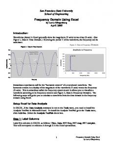
ABSTRACT In this paper a computational alternative to classify lung nodules inside CT thorax images in the frequency domain is presented. After image acquisition, a region of interest is manually selected. Then, the spectrums of the two dimensional Discrete Cosine Transform (2D-DCT) and the two dimensional Fast Fourier Transform (2D-FFT) were calculated. Later, two statistical texture features were extracted from the histogram computed from the spectrum of each CT image. Finally, a support vector machine with a radial basis function as a kernel was used as the classifier. Seventy five tests with different diagnosis and number of images were used to validate the methodology presented. After experimentation and results, ten false negatives (FN) and two false positives (FP) were obtained, and a sensitivity and specificity of 96.15% and 52.17% respectively. The total preciseness obtained with the methodology proposed was 82.66%. Keywords: Lung nodule detection (LND), Support Vector Machine (SVM), Discrete Cosine Transform (DCT), Fast Fourier Transform (FFT), Computer Tomography (CT). 1. INTRODUCTION Lung cancer has become one of the leading causes of death worldwide. It is estimated that 85% of lung cancer cases are related to smoke. Smokers are about 10 times more exposed to get lung cancer than those who are not smokers [1]. The success of a treatment for cancer of any type depends on a opportune diagnosis, which in this case leads to the identification of lung nodules. This nodules are small lesions that may or may not calcified, usually spherical shaped or with irregular edges. In M´exico 8,255 cases of lung cancer are reported annually. Between 80% and 97% of all the patients diagnosed with lung cancer died in less than a year after the cancer was detected. The 95% of cases are diagnosed in stage III when the treatment depends on the location of lung cancer and stage IV when the cure is not possible. Due to this disease in M´exico every day 22 people died [2]. Unfortunately, lung cancer tends to be undetected at early stages. Typically, lung cancer is detected when it has evolved This project was partially supported by FOMIX CHIH-2009-C01117569.
978-1-4673-0382-8/12/$31.00 ©2012 IEEE
and reached a stage where it becomes more difficult to treat. So it is of highest importance to increase the possibility of an early detection. The detection of lung nodules can provide the help necessary for the patient to receive an opportune treatment. Therefore, this research focuses on the classification of lung nodules by transforming the CT images to frequency domain and classifying it using a support vector machine. This paper is organized as follows: in section 2 the works related to this research are mentioned. Section 3 explains the proposed methodology for lung nodules detection and classification. Test and experimental results are presented in section 4. The conclusions and further works are presented in section 5.
2. RELATED WORKS In recent years, researchers have been working to investigate the issue of cancer. The main interest is to provide new methods and techniques that can help the radiologists to offer a better diagnosis. The approach of this researches is to avoid invasive methods to detect cancer at early stages and consequently give a longer life expectancy to the patient with cancer. The work proposed by [3], presents a technique which consists of several steps, including lung segmentation, improvement of the candidates to be lung nodules, feature extraction of the voxels and the voxels classification using support vector machines (SVM). Two sets of data of lung nodules were used to evaluate the system performance. A database of 32 patients with lung nodules and a SVM with two kernels (polynomial and Gaussian) were implemented to compare the results. The kernel with better perform was the Gaussian also known as Radial Basis Function (RBF). The sensitivity obtained was 87.5% and the specificity of 92.83%. In the classification of lung nodules also exist hybrid classifiers as the proposed by [4]. To determine if there are lung nodules inside the images, an stage of feature extraction based on the form was implemented, with the disadvantage that some blood vessels were classified as lung nodules. At the second stage the texture features were calculated to discriminate the blood vessels. The classifier used was a SVM with Rule-Based System individually. In order to validate the methodology a comparison of the SVM and the Rules-Based System was made, by combining these two methods a specificity of 92% was obtained. In Table 1 some of the latest works related to the lung nodule detection, including its classifier and sensitivity, are shown.
870
Table 1. Chronology of the works developed in the last years in lung nodule detection. Author Yang Liu et al. [3] Zhenghao Shi et al. [5] Yang Liu et al. [6] Zhang Jing et al. [4] Farag A. et al. [7] Anand S.K.V. [8] S.Aravind Kumar et al. [9] Zinovev, Dmitriy at al. [10]
Classifier Support vector machine radial basis function Neural networks Support vector machine polinomial Support vector machine ruled based system Non-parametric template matching Neural network / inference and forecasting Fuzzy system Decision trees
Sensitivity 87.50% 60% 94% N/A
3.2. Region of interest The examinations files obtained at the image acquisition stage contain several differences between them, in some files the CT images contain the information in a circle while the others not. To eliminate the differences between the images a region of interest (ROI) was manually defined. Considering the limits of a circle the ROI were marked, leaving inside the circle the relevant information and making it black outside. After this stage, all the CT images used preserve the important information inside the circle area as it is shown in Figure 2.
85.22% 89.6% 90% 69%
3. MATERIALS AND METHODS The stages of the proposed methodology to solve the problem statement are: 1) Image acquisition, 2) Region of interest, 3) Frequency domain, 4) Statistical texture features extraction, 5) Attribute selection, 6) Classification and 7) Diagnostic. In Figure 1 a scheme of the methodology proposed is shown.
Image acquisition
Region of interest
Frequency domain
Attribute selection
Statistical texture features extraction
yes Classification
Presence of lung nodules
no Absence of lung nodules
Fig. 1. Scheme of the proposed methodology.
a)
b)
Fig. 2. Region of interest extraction: a) Original CT image and b) CT image after ROI extraction.
3.3. Frequency domain A transformation refers to the change of an image representation, (i.e.) from the spatial domain to the frequency domain. At this stage, two transformations which have good energy compaction abilities were used: a) The two dimensional Discrete Cosine Transform (2D-DCT) and b) the two dimensional Fast Fourier Transform (2D-FFT). The 2D-DCT is the key tool in the format compression JPEG and the 2D-FFT is an important tool that is used to decompose an image into sine and cosine components. Both transforms can compact the energy of an image to the the upper left corner. 3.3.1. Fast Fourier Transform The FFT was used to transform each CT image from spatial to frequency domain. For reasons of speed the 2D-FFT the algorithm was used. The Fourier transform of an image computes the frequency components, the position of each component reflects its frequency: Low frequencies are near to the origin and high frequencies are further away [11]. Equation 1 shows how to compute the 2D-FFT of a CT image and Equation 2 shows a way to compute the Fourier spectrum. In Figure 3 the Fourier spectrum of a CT image is shown.
F (p, q) =
3.1. Image acquisition
M −1 N −1 X X
f (m, n)e−j(2π/M ) e−j(2π/N )qm
(1)
m=0 n=0
The images analyzed were Computer Tomography (CT) of thorax. The dataset were acquired from the National Biomedical Imaging Archives (NBIA) and Early Lung Cancer Action Project (ELCAP). The grayscale images have a size of 512 × 512 pixels with the format Digital Imaging and Communications in Medicine (DICOM) which is the standard for medical image. The images were grouped in examination files which contain an average of 200 CT image slices. Each examination file of the data base was obtained by a different scanner.
1
|F (p, q)| = [R2 (p, q) + I 2 (p, q)] 2
(2)
where f (m, n) are the spatial components, M and N are the row and column size of f (m, n), F (p, q) are the spectral components , R(p, q) is the real part (cosine) and I(p, q) is the
871
imaginary part (sine) of F (p, q) and |F (p, q)| is the magnitude of 2D-FFT.
a) a)
b)
Fig. 4. Cosine spectrum. a) Original CT image and b) CT image after compute DCT spectrum.
b)
Fig. 3. Fourier spectrum. a) Original CT image and b) CT image after compute 2D-FFT spectrum. Six texture features that were defined in [13] such as average gray level (Equation 4), standard deviation, smoothness, third moment (Equation 5), uniformity and entropy were computed. Average gray level
3.3.2. Discrete Cosine Transform The two dimensional Discrete Cosine Transform (2D-DCT) is an important tool for data compression. Which makes it so useful is that it takes correlated input data and concentrates its energy in just the first few transform coefficients [11]. The position of each component reflects its frequency: Low frequency components are near the upper left corner and high frequency components are further away. Equation 3 shows how to compute the DCT. In Figure 4 the DCT spectrum of a CT image is shown.
F (u, v) = αu αv
PM −1 PN −1 m=0
n=0
f (m, n)cos
(3)
where
αu =
1 √ ,u = 0 M
r
L−1 X
zi p(zi )
(4)
(zi − m)3 p(zi )
(5)
i=0
Third moment µ3 =
L−1 X i=0
π(2m + 1)u π(2n + 1)v cos 2M 2N
0≤u≤M −1 0≤v ≤N −1
m=
where zi is a random variable which indicates intensity. P (z) is the histogram of the intensity levels on a region. L is the number of possible intensity levels. The 2D-FFT spectrum |F (p, q)| and the 2D-DCT spectrum F (u, v) of each image was divided in 4 frequency bands. The respective sizes were 512 × 512, 256 × 256, 128 × 128 and 64 × 64. Therefore, 6 features were extracted from each frequency band to get a total of 24 features. In Figures 5 and 6 the frequency bands that were analyzed as well as their sizes are shown. The frequency bands were built based on the area in which the 2D-DCT and 2D-FFT concentrates the energy.
2 ,1 ≤ u ≤ M − 1 M
y
y
0
0
256
256
and
αv =
1 √ ,v = 0 N
r
2 ,1 ≤ v ≤ N − 1 N
512
256
x 512
512
256
a) where f (m, n) are the spatial components, M and N are the row and column size of f (m, n) and F (u, v) are the spectral components.
Every one has their own interpretation as to the nature of texture; there is no mathematical definition of texture, it simple exists [11]. In an image the texture is characterized by the spatial distribution of gray levels in a neighborhood. Therefore, the texture can not be defined by a point. The histogram of an image allows at a glance, get a rough idea of the distribution of gray levels and contrast [12]. In this stage, statistical texture features were extracted from the histogram of each CT image.
b)
y
3.4. Statistical texture features extraction
y
0
0
256
256
512
x 512
256
c)
x 512
512
256
x 512
d)
Fig. 5. 2D-FFT frequency bands. a) Frequency band of 512 × 512, b) Frequency band of 256 × 256, c) Frequency band of 128 × 128 and d) Frequency band of 64 × 64.
872
y
y
0
0
256
256
512
x 512
256
many support vectors needs to be stored and and the algorithm overfits. If it is too small and underfitting is obtained [17]. K(xt , x) = C · exp[
512
256
a)
x 512
b)
y
y
0
0
256
256
512
x 512
256
512
256
−||xt − x||2 ] σ2
(6)
The SPIDER toolbox [18] was used to define the value of σ, it is an object-oriented environment for machine learning in Matlab. The centroids were calculated using WEKA with the algorithm k-means clustering which groups data according to the general average of each feature. In order to train the SVM-RBF a set of 61 CT images were use, 36 CT images with lung nodules and 25 CT images without lung nodules. In Figure 7 and 8 a graphic for the vectors of each transform are shown.
x 512 0.5
c)
d)
yes no
0 −0.5
Fig. 6. 2D-DCT frequency bands. a) Frequency band of 512 × 512, b) Frequency band of 256 × 256, c) Frequency band of 128 × 128 and d) Frequency band of 64 × 64.
−1 −1.5 −2 −2.5
3.5. Attribute selection
−3 −3.5
After the computation of 24 statistical texture features, different algorithms as BestFirst, GeneticSearch and GreedyStepwise was tested to measure the relevance of each feature and to reduce the feature set. The feature set of 24 statistical texture features were reduced to 2 statistical texture features: average gray level and third moment. This step was made using the Waikato Environment for Knowledge Analysis (WEKA) software [14]. Table 2 summarizes this stage, the most important features and the frequency band in which they are located for each transform are shown.
−4 −4.5 127
128
129
130
131
132
133
134
135
136
Fig. 7. Vectors: average gray level and third moment of 2D-DCT.
5 yes no
Table 2. Results after the selection of the best attributes. Transform DCT DCT FFT FFT
Feature Average Gray level Third moment Average Gray level Third moment
0
Frequency band 512 64 512 512
−5
−10
−15
−20
−25 120
130
140
150
160
170
180
3.6. Classification After attribute selection, the classification stage was made using a Support Vector Machine (SVM). SVM were developed by Vapnik in 1995 [15] for the classification problem, but the present form of SVM for regression was developed in the laboratories of AT&T by Vapnik in 1997 [16]. The theoretical characteristics of SVM are defined for classification problems with two classes. since typically, the features of interest can not be linearly separable, instead of fitting a nonlinear function, one trick is to use a kernel. The kernel used in this research was a Radial Basis Function (RBF). Equation 6 defines a spherical kernel. Where xt is the center, x is the input feature, σ is given by the user and C is the penalty factor. It is critical that a proper penalty factor value is chosen, if it is too large, then a high penalty for nonseparable points is obtained,
Fig. 8. Vectors: average gray level and third moment of 2D-FFT.
873
3.7. Diagnostic
Kernel Function: rbf_kernel 5
Diagnostic is the process by which a disease is identified, in this case to detect if there are lung nodules inside the CT images or not. For all the images 2 statistical texture features were computed to obtain the support vectors, the optimal hyperplane, the penalty factor and the centroids. The SVM-RBF training step was performed using these data. In Figure 9 a graphic with trained support vectors is shown. An image is classified into one of two groups: 1) Presence of lung nodules (red) and 2) Absence of lung nodules (green).
yes (training) yes (classified) no (training) no (classified) Support Vectors
0
−5
−10
−15
−20
−25 120
130
140
150
160
170
180
5 yes no Support Vectors 0
Fig. 11. Tested vectors: Gray level average and third moment of 2D-FFT.
−5
−10
−15
−20
−25 120
130
140
150
160
170
180
Fig. 9. Trained vectors: average gray level and third moment 2D-FFT.
When comparing the test results to evaluate and diagnosis reference there are four different posibilities: False Positive (FP) indicates a disease when in fact does not exist, False Negative (FN) indicates no disease when in fact does exist, True Positive (TP) indicates a disease and True Negative (TN) indicates no disease. These four possibilities can be summarized in a 2 x 2 contingency table in order to compare the results obtained with the proposed algorithm and the radiologist. In Tables 3 and 4 the contingency matrix using the 2D-DCT the 2D-FFT respectively are shown.
Table 3. 2D-DCT contingency table. Presence True positive True negative Total
4. EXPERIMENTS AND RESULTS The system was trained using a total of 61 CT images, 36 CT images with lung nodules and 25 CT images without lung nodules. The ability of the system to detect lung nodules inside an image was validated by the Professional Technical Radiology Antonio Estrada Barrientos, who works at the Center for Advanced Imaging SC. The methodology was tested and validated with a clinical data set of 75 thoracic CT examination files (involving 15,600 CT slices) which contains 52 CT scans with lung nodules. In Figures 10 and 11 the results of overall test performance are shown.
50 12 62
Absence False positive False negative
11 2 13
Total 61 14 75
Table 4. 2D-FFT contingency table. Presence True positive True negative Total
51 11 62
Absence False positive False negative
10 3 13
Total 61 14 75
Kernel Function: rbf_kernel 0.5 yes (training) yes (classified) no (training) no (classified) Support Vectors
0 −0.5
Diagnostic test should ideally have a sensitivity and specificity as close to 100% as possible [19]. The specificity (Equation 7) of a test indicates the probability of obtaining a negative result when the individual has the disease. The sensitivity (Equation 8) of a diagnostic test is the probability of obtaining a positive result when the individual has the disease. Preciseness (Equation 9) is the proportion of valid results from all tests performed.
−1 −1.5 −2 −2.5 −3 −3.5 −4 −4.5 127
128
129
130
131
132
133
134
135
specif icity =
TP TP + FN
(7)
sensitivity =
TN TN + FP
(8)
TP + TN TP + FP + TN + FN
(9)
136
Fig. 10. Tested vectors: Gray level average and third moment of 2D-DCT.
preciseness =
874
support vector machines,” IEEE International Conference on Computer Application and System Modeling (ICCASM), vol. 10, pp. 118 – 121, october 2010.
where TP are the true positive, TN are the true negative, FP are the false positive and FN are the false positive, all obtained from the contingency table. Finally, in Table 5 the results of sensitivity, specificity and preciseness of the proposed methodology using the 2D-DCT and 2D-FFT are shown.
[7] Farag A., Graham J., Elshazly S., and Farag A., “Statistical modeling of the lung nodules in low dose computed tomography scans of the chest,” 17th IEEE International Conference on Image Processing (ICIP), pp. 4281 – 4284, september 2010.
Table 5. Final results. Transform 2D-DCT 2D-FFT
Sensitivity 96.15% 94.44%
Specificity 52.17% 52.38%
Preciseness 82.66% 82.66%
[8] Anand S.K.V., “Segmentation coupled textural feature classification for lung tumor prediction,” IEEE International Conference on Communication Control and Computing Technologies (ICCCCT), pp. 518 – 524, october 2010. [9] Kumar S.A., Ramesh J., Vanathi P.T., and Gunavathi K., “Robust and automated lung nodule diagnosis from ct images based on fuzzy systems,” IEEE International Conference on Process Automation, Control and Computing (PACC), pp. 1 – 6, July 2011.
5. CONCLUSIONS In this paper a methodology for lung nodule classification was presented. The results were favorable, statistical texture feature extraction from 2D-DCT and 2D-FFT spectrum and SVM-RBF as a classifier indicate whether a CT image has lung nodules or not. The ability of the system to detect lung nodules inside an image was validated by the Professional Technical Radiology Antonio Estrada Barrientos, who works at the Center for Advanced Imaging SC. The methodology was validated on a clinical data set of 75 thoracic CT examination files (involving 15,000 CT slices) that contains 52 CT examination files with lung nodules. In the analysis of CT images in the frequency domain the most important features were the average gray level and the third moment. The SVM-RBF presented good results in the training and classification stages. The results show that the proposed methodology successfully detects nodules of 2 millimeters to 3 centimeters in diameter. The 2D-DCT showed better sensitivity compared with the 2D-FFT. In the future the algorithm will be tested using different classifiers and transforms such as neural networks or boosting and Discrete Wavelet Transform (DWT) or Contourlet Transform.
[10] Zinovev Dmitriy, Feigenbaum Jonathan, Furst Jacob, and Raicu Daniela, “Probabilistic lung nodule classification with belief decision trees,” Annual International Conference of the IEEE, Engineering in Medicine and Biology Society, EMBC, pp. 4493 – 4498, September 2011. [11] Mark Nixon and Alberto Aguado, Feature extraction and image processing, Academic Press, second edition, 2008. [12] Anil K. Jain, Fundamentals of Digital Image Processing, Prentice Hall Information and Systems Science Series, 1989. [13] Rafael C. Gonz´alez and Richard E. Woods, Digital Image Processing Using Matlab, Prentice Hall, first edition, 2004. [14] Mark Hall, Eibe Frank, Geoffrey Holmes, Bernhard Pfahringer, Perter Reutemann, and Ian H. Witten, “The weka data mining software,” SIGKDD Explorations Newsletter, vol. 11, no. 1, pp. 10–18, 2009.
6. REFERENCES
[15] Vladimir Vapnik, The nature of statistical learning theory, Springer, second edition, 1999.
[1] Mylene T. Truong, Badley S. Sabloff, and Jane P. Ko, “Multidetector ct of solitary pulmonary nodules,” Thoracic Surgery Clinics, vol. 20, no. 1, pp. 9–23, February 2010.
[16] Vapnik V N, Golowich S, and Smola A, “Support vector method for function approximation, regression, estimation and signal processing,” Advances in Neural Information Processing Systems, pp. 281–287, 1997.
[2] Instituto Nacional de Estad´ıstica y Geograf´ıa (INEGI), “Estad´ısticas a prop´osito del d´ıa mundial contra del c´ancer” datos nacionales,” pp. 1–3, February 2007.
[17] Ethem Alpaydin, Introduction to Machine Learning, The MIT Press, second edition, 2010.
[3] Yang Liu, Jinzhu Yang, Dazhe Zhao, and Jiren Liu, “Computer aided detection of lung nodules based on voxel analysis utilizing support vector machines,” International Conference on Future BioMedical Information Engineering, (FBIE), pp. 90 – 93, december 2009. [4] Zhang Jing, Li Bin, and Tian Lianfang, “Lung nodule classification combining rule-based and svm,” IEEE Fifth International Conference on Bio-Inspired Computing: Theories and Applications (BIC-TA), pp. 1033 – 1036, september 2010.
[18] Jason Weston, Andre Elisseeff, G¨okhan Bakir, and Fabian Sinz, “The spider,” . [19] M. J. Burgue˜no, J. L. Garc´ıa-Bastos, and J.M. Gonz´alezBuitrago, “Las curvas roc en la evaluaci´on de las pruebas diagn´osticas,” Med Clin, vol. 104, pp. 661–670, december 1993.
[5] Zhenghao Shi, Suzuki K., and Lifeng He, “Reducing fps in nodule detection using neural networks ensemble,” IEEE Second International Symposium on Information Science and Engineering (ISISE), pp. 331 – 333, december 2009. [6] Yang Liu, Jinzhu Yang, Dazhe Zhao, and Jiren Liu, “A method of pulmonary nodule detection utilizing multiple
875