M-9 Linear Programming in MATLAB

MCS 320

Introduction to Symbolic Computation

Spring 2003

9. Linear Programming in MATLAB One of the most widespread commercial applications of scientific computation is linear programming.

9.1 An optimization problem Suppose a farmer has 75 acres to plant and must decide how much farm land to devote to crop x or crop y. Crop x brings in more revenue than y, as can be seen from the profit function P (x, y): P (x, y) = 143x + 60y. In maximizing the profit P (x, y), all should be devoted to crop x, but farming is not that simple. There are additional constraints (other than x + y ≤ 75). For instance, crop x requires more storage space than crop y, and if the total storage is limited to 4,000, then we have to take the following constraint 110x + 30y ≤ 4, 000 into account. The crops just do not grow for free. As the farmer cannot spend more than 15,000 to grow the crops, the third constraint takes the form 120x + 210y ≤ 15, 000. In addition to the trivial constraints x ≥ 0 and y ≥ 0, our problem is summarized into: max 143x + 60y x,y  x+ y    110x + 30y subject to 120x + 210y    x ≥ 0, y ≥ 0

≤ 75 ≤ 4, 000 ≤ 15, 000

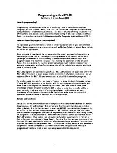
Since there are only two unknowns involved, we may graph all constraints: >> x = 0 : 80; % range for graph enter >> y1 = max(75 − x, 0); % x + y ≤ 75 farm land enter >> y2 = max((4000 − 110 ∗ x)/30, 0); % 110x + 30y ≤ 4000 storage enter >> y3 = max((15000 − 120 ∗ x)/210, 0); % 120x + 210y ≤ 15000 expenses enter >> ytop = min([y1; y2; y3]); % array of minima enter >> area(x, ytop); % filled area plot enter The shaded area enclosed by the constraints is called the feasible region, which is the set of points satisfying all the constraints. If this region is empty, then the problem is said to be infeasible, and it has no solution. The lines of equal profit p are given by p = 143x + 60y. If we fix p to, say 50, then all points (x, y) which satisfy 143x + 60y yield the same profit 50. >> hold on; >> [u v] = meshgrid(0 : 80, 0 : 80); >> contour(u, v, 143 ∗ u + 60 ∗ v); >> hold of f ;

enter enter enter enter

To find the optimal solution, we look at the lines of equal profit to find the corner of the feasible region which yields the highest profit. This corner can be found at the farthest line of equal profit which still touches the feasible region. Jan Verschelde, April 25, 2003

UIC, Dept of Math, Stat & CS

MATLAB Lecture 9, page 1

MCS 320

Introduction to Symbolic Computation

Spring 2003

9.2 The command linprog The command linprog from the optimization toolbox implements the simplex algorithm to solve a linear programming problem in the form min f ∗ x x

subject to A ∗ x ≤ b where f is any vector and the matrix A and vector b define the linear constraints. So our original problem is translated into the format min − 143x − 60y

max 143x + 60y

x,y

x,y

subject  to x+ y    110x + 30y  120x + 210y   x ≥ 0, y ≥ 0

≤ 75 ≤ 4, 000 ≤ 15, 000

subject  to    1 1 75  110 30  · ¸  4, 000       120 210  x ≤  15, 000    y    −1   0  0 0 −1 0

Observe the switching of signs to turn the max into a min and to deal with the ≥ constraints. Now we are ready to solve the problem. First we set up the vectors and matrices: >> f = [−143 − 60] >> A = [120 210; 110 30; 1 1; −1 0; 0 − 1] >> b = [15000; 4000; 75; 0; 0]

enter enter enter

The optimization toolbox has the command linprog: >> linprog(f, A, b) % optimize enter >> −f ∗ ans % compute profit enter The latest versions of MATLAB have the command simlp, which is very much like linprog.

9.3 Assignments 1. Suppose General Motors makes a profit of $100 on each Chevrolet, $200 on each Buick, and $400 on each Cadillac. These cars get 20, 17, and 14 miles a gallon respectively, and it takes respectively 1, 2, and 3 minutes to assemble one Chevrolet, one Buick, and one Cadillac. Assume the company is mandated by the government that the average car has a fuel efficiency of at least 18 miles a gallon. Under these constraints, determine the optimal number of cars, maximing the profit, which can be assembled in one 8-hour day. Give all MATLAB commands and the final result. 2. Consider the following optimization problem: min 2x + y x,y

subject  to x+ y    x + 3y x− y    x ≥ 0,

≥ 4 ≥ 12 ≥ 0 y≥0

(a) Use MATLAB to graph the constraints. (b) Use linprog to compute the solution.

Jan Verschelde, April 25, 2003

UIC, Dept of Math, Stat & CS

MATLAB Lecture 9, page 2