These notes cover a lot of the 2008-2009 Ma432 Classical Field Theory course
given by Dr Nigel ... 4.3.1 Stress-energy tensor for electromagnetic field .
Ma432 Classical Field Theory Notes by Chris Blair These notes cover a lot of the 2008-2009 Ma432 Classical Field Theory course given by Dr Nigel Buttimore (replaced by Ma3431 Classical Field Theory and Ma3432 Classical Electrodynamics, the former corresponding to at least the first four sections of these notes). The emphasis is mostly on the Lagrangian formulation of classical electrodynamics and the solution of Maxwell’s equations by Green’s function methods. They are probably slightly suspect, particularly with regard to indices and brackets (and no doubt contain other more unsettling errors). I am told that Dr Buttimore has changed his units from those in these notes, so use at your own discretion.
Contents 1 Simple field theory 1.1 Introduction to field theory . . . . . . . . . . . . . . . . . . . . . . . . . . . 1.2 Field theory as a continuum limit . . . . . . . . . . . . . . . . . . . . . . . . 1.3 Euler-Lagrange equations . . . . . . . . . . . . . . . . . . . . . . . . . . . . .
3 3 3 4
2 Special relativity 2.1 Rapidity . . . . . . . . . . . . . . . . . . . . . . . . . . . . . . . . . . . . . . 2.2 Tensor notation . . . . . . . . . . . . . . . . . . . . . . . . . . . . . . . . . .
6 6 7
3 Covariant field theory 3.1 Relativistic free particle action . . . . 3.2 Relativistic interactions . . . . . . . . 3.3 Electromagnetic field tensor . . . . . 3.4 Maxwell’s equations . . . . . . . . . . 3.5 Four-current and charge conservation
. . . . .
. . . . .
. . . . .
. . . . .
. . . . .
. . . . .
. . . . .
. . . . .
4 Noether’s theorem 4.1 Derivation . . . . . . . . . . . . . . . . . . . . . . . 4.2 Examples . . . . . . . . . . . . . . . . . . . . . . . 4.3 Stress-energy tensor . . . . . . . . . . . . . . . . . . 4.3.1 Stress-energy tensor for electromagnetic field 5 Solving Maxwell’s equations 5.1 Time-independent solutions . . . . . . . . . . . . 5.1.1 Green’s function . . . . . . . . . . . . . . 5.1.2 Magnetostatic and electrostatic potentials 5.2 Time-dependent solutions . . . . . . . . . . . . . 1
. . . .
. . . . .
. . . .
. . . .
. . . . .
. . . .
. . . .
. . . . .
. . . .
. . . .
. . . . .
. . . .
. . . .
. . . . .
. . . .
. . . .
. . . . .
. . . .
. . . .
. . . . .
. . . .
. . . .
. . . . .
. . . .
. . . .
. . . . .
. . . .
. . . .
. . . . .
. . . .
. . . .
. . . . .
. . . .
. . . .
. . . . .
. . . .
. . . .
. . . . .
. . . .
. . . .
. . . . .
10 10 11 12 13 15
. . . .
17 17 18 20 20
. . . .
22 22 22 23 23
5.2.1 5.2.2 5.2.3 5.2.4 5.2.5 5.2.6
Green’s function . . . . . . . . . . . . . . . . . . . . . . . . . . . . . Lienard-Wiechart potentials . . . . . . . . . . . . . . . . . . . . . . . Electromagnetic fields from Lienard-Wiechart potentials: method one Electromagnetic fields from Lienard-Wiechart potentials: method two Properties of the electromagnetic fields due to a moving charge . . . . Local form of the electromagnetic fields due to a moving charge . . .
24 26 28 29 30 31
6 Power radiated by accelerating charge
33
7 Bibliography
34
Notes for Classical Field Theory
1 1.1
Section 1: Simple field theory
Simple field theory Introduction to field theory
You are probably already familiar with the notion of electric and magnetic fields. Loosely speaking, a field in a physics is a physical quantity defined at every point of space and time, which can be valued as a single number (scalar field), a vector (vector field, such as electromagnetism and gravity), or as a tensor. We will restrict ourselves to the study of the electric and magnetic fields, and do so in a unified manner consistent with special relativity. The methods we use are based in the Lagrangian approach to classical mechanics. Recall that in classical mechanics the Lagrangian L was defined as L = T − V where T and V are the kinetic and potential energies of the R system in question. The action of the system was defined to be the quantity S = Ldt, and the equations of motion of the system were found from the principle of least action, which states that the true time evolution of the system is such that the action is an extremum. The equations of motion (known as the Euler-Lagrange equations) were thus derived from R the condition δS = δ Ldt = 0. In studying fields which take on different valuesRat different space points it is convenient to express the Lagrangian itself as an Rintegral, L = d3 x L, where L is called the Lagrangian density. The full action is then S = dtd3 x L. Note that when we approach this from the special relativistic point of view the separate time and space components will be unified into a single package.
1.2
Field theory as a continuum limit
To begin, let us show how a simple field theory may be derived by taking the continuum limit of a system of N particles on a spring with spring constant k. Let the particles have equilibrium positions a, 2a, . . . N a and denote the deviation of the ith particle from its equilibrium by φi . The force on the ith particle is ( +k(φ − φ ) i=1 2
Fi =
1
−k(φi − φi−1 ) + k(φi+1 − φi ) 1 < i < N −k(φN − φN −1 ) i=N
The Lagrangian is L=T −V =
N X 1 i=1
2
mφ˙ 2i −
N X 1 i=1
2
k(φi+1 − φi )2
and the equations of motion are mφ¨i = −k(φi − φi−1 ) + k(φi−1 − φi )
1 0. This condition is imposed as z 0 = x0 − x00 = c(t − t0 ), and so positive z 0 ensures that contributions to the Green’s function and hence to the potential Aµ only come from events that occur at times t0 < t, i.e. events in the past. Thus causality is ensured. Now, the poles of the integrand are ±k and so lie on the real axis. To avoid them, we displace our contour by an infinitesimal amount i� so that it lies just in the upper-half plane (formally we should let � → 0 at the end). Our contour of integration Γ then looks like: Im k0
Re k0 −k
k
Γ
R
We than have
0
e−ik0 z dk0 2 = k0 − k 2 Γ
I
0
R
e−ik0 z dk0 2 + k0 − k 2 −R
Z
−iϕ
Z semi-circle
0
e−ik0 z k02 − k 2
Now on the semicircle we can write k0 = Re = R cos ϕ − iR sin ϕ, so that the integral becomes an integral over ϕ from 0 to π. So we have Z Z π 0 e−ik0 z 1 0 0 = −i dϕ Reiϕ e−Rz sin ϕ−iRz cos ϕ 2 −2iϕ 2 2 R e − k2 semi-circle k0 − k 0 24
Notes for Classical Field Theory
Section 5: Solving Maxwell’s equations
and sin ϕ ≥ 0 for this range of ϕ, hence the integrand goes to zero as R → ∞, as required. The value of the k0 integral we are interested in will hence be given by the −2πi times the sum of the residues inside the contour. The residues are: 0
e−ikz e−ik0 z = lim (k0 − k) k0 →k (k0 − k)(k0 + k) 2k 0
0
eikz e−ik0 z =− lim (k0 + k) k0 →−k (k0 − k)(k0 + k) 2k hence
Z
∞
dk0 −∞
0
� 1 πi � ikz0 −ik0 z 0 −ikz 0 e = e − e Θ(z 0 ) 2 2 k0 − k k
where the Heaviside function
( 1 z0 > 0 Θ(z ) = 0 z0 < 0 0
is added as the residues only contribute for positive z 0 . So we now have Z � 0 � Θ(z 0 ) µ 3 i~k·~ z1 ikz −ikz 0 D(z ) = πi d k e e − e (2π)4 k Z � � Z 2π Z π ∞ Θ(z 0 ) 21 ikz 0 −ikz 0 i dk k e −e dφ dθ sin θ eikz cos θ = 16π 3 0 k 0 0 upon switching to polar coordinates and choosing the coordinate frame such that the k 3 axis makes an angle of θ with ~z, and letting z = |~z|. Integrating over the angles, we get Z ∞ � 0 � � eikz e−ikz � Θ(z 0 ) ikz µ −ikz 0 i dk k e − D(z ) = −e 8π 2 ikz ikz 0 � � 0 Z ∞ Θ(z ) ik(z 0 +z) −ik(z 0 +z) ik(z 0 −z) −ik(z 0 −z) dk e +e −e −e =− 2 8π z 0 but if we let k 7→ −k Z ∞ dk e
−ik(z 0 +z)
0
Z =
−∞
ik(z 0 +z)
d(−k)e
Z
0
=
dk eik(z
0 +z)
−∞
0
hence Θ(z 0 ) D(z ) = − 2 8π z µ
∞
� � Θ(z 0 ) � 0 0 dk eik(z+z ) − eik(z −z) = δ(z 0 − z) − δ(z 0 + z) 4πz −∞
Z
remembering the integral representation of the delta function. Owing to the Heaviside function only the first delta function will contribute, so Dret (z µ ) =
Θ(z 0 ) 0 δ(z − z) 4πz 25
Notes for Classical Field Theory
Section 5: Solving Maxwell’s equations
The subscript signifies that this is the retarded Green’s function (that is, the Green’s function resulting from the contribution of events in the past). We can put the Green’s function in covariant form using δ(zµ z µ ) = δ([z0 − z][z0 + z]) = as δ(ab) =
δ(a) |b|
+
δ(b) . |a|
δ(z0 − z) δ(z0 + z) + |z0 + z| |z0 − z|
Hence Θ(z 0 )δ(zµ z µ ) = Θ(z 0 )
δ(z0 − z) δ(z0 − z) = Θ(z 0 ) |z0 + z| |2z|
and so
Θ(z 0 ) δ(zµ z µ ) 2π Recalling that z µ = xµ − x0µ we can state our final results for the Green’s function as Dret (z µ ) =
Dret (xµ − x0µ ) =
Θ(x0 − x00 ) δ(x0 − x00 − |~x − x~0 |) 4πz
and in covariant form, Dret (xµ − x0µ ) =
Θ(x0 − x00 ) δ([xµ − x0µ ][xµ − x0µ ]) 2π
Note that if we had taken z 0 < 0 and closed our contour in the upper half-plane (with poles displaced upwards) we would have obtained the advanced Green’s function Dadv (xµ − x0µ ) =
5.2.2
Θ(x00 − x0 ) δ(x0 − x00 + |~x − x~0 |) 4πz
Lienard-Wiechart potentials Of night and light and the half-light. W.B. Yeats, “He Wishes For The Cloths Of Heaven”
We can now work out the potentials Aµ that solve the Maxwell equation ∂µ ∂ µ Aν = They are given by Z 4π µ σ A (x ) = d4 x0 Dret (x − x0 )J µ (x0σ ) c where dx0σ J µ (x0σ ) = e 0 δ 3 (~x0 − ~x0e (t)) dt or in covariant form Z dx0σ 4 0σ µ 0σ J (x ) = ec dτ δ (x − x0σ e (τ )) dτ 26
4π ν J . c
Notes for Classical Field Theory
Section 5: Solving Maxwell’s equations
as integrating over τ and using that δ(f (τ )) =
X δ(τ − τi ) |f 0 (τi )|
i:f (τi )=0
we have
dx0σ 3 0 J (x ) = ec δ (~x − ~x0e (t)) dτ τ 0 µ
0σ
�
dx00 dτ
00
00
�−1
0σ
τ0 0σ
dt dt dt |τ 0 = c dτ |τ 0 and dxdτ |τ 0 = dxdt dτ |τ 0 so this reduces where x00 − x0e (τ 0 ) = 0. Now, dxdτ |τ 0 = dxdt dτ to the local form. So substituting this in, we have Z 4π dx0σ 4 0σ Θ(x0 − x00 ) µ σ A (x ) = δ([xσ − x0σ ][xσ − x0σ ])ec δ (x − x0σ dτ d4 x0 e (τ )) c 2π dτ Z = 2e dτ Θ(x0 − x0e )δ([xσ − xeσ (τ )][xσ − xσe (τ )])V µ (τ ) µ
e . Now, we need the roots of the argument of the delta where we have written V µ ≡ dx dτ function: [xσ − xeσ (τ )][xσ − xσe (τ )] = 0 ⇒ (x0 − xe0 (τ ))2 − |~x − ~xe (τ )|2 = 0
There are two possibilities: x0 − xe0 (τ ) = ±|~x − ~xe (τ )| The Heaviside function constrains us to choose the positive option. We see that the unique root of [xσ − xeσ (τ )][xσ − xσe (τ )] = 0 which ensures causality is given by the retarded time τ0 : x0 − xe0 (τ0 ) = |~x − ~xe (τ0 )| Physically, the retarded time gives the unique time at which the charged particle intersects the past light-cone of the observation point. Now, as d d [xσ − xeσ (τ )][xσ − xσe (τ )] = −2[xσ − xeσ (τ )] xσe (τ ) dτ dτ We then have that Θ(x0 − x0e )δ([xσ − xeσ (τ )][xσ − xσe (τ )]) =
δ(τ − τ0 ) 2[xσ − xeσ (τ0 )]V σ (τ0 )
so, writing Rσ = xσ − xσe (τ0 ), we have µ V (τ ) Aµ (xσ ) = Rσ (τ )V σ (τ )
τ0
Note that the retarded time is in this notation defined by Rσ (τ0 )Rσ (τ0 ) = 0 and that then ~ = |~x − ~xµe (τ0 )|. R0 = R = |R| 27
Notes for Classical Field Theory 5.2.3
Section 5: Solving Maxwell’s equations
Electromagnetic fields from Lienard-Wiechart potentials: method one
We wish to evaluate the electromagnetic fields F µν = ∂ µ Aν − ∂ ν Aµ arising from the motion of a charged particle. Consider the integral expression for the potential Z ν σ A (x ) = 2e dτ Θ(x0 − x0e )δ([xσ − xeσ (τ )]2 )V ν (τ ) We will differentiate this with respect to xµ . First, note that ∂µ Θ(x0 − x0e ) = δ(x0 − x0e ) and this will give a term δ(−|~x − ~xe (τ )]2 ) which only contributes for ~x = ~xe (τ ) and can be neglected. Thus we have Z µ ν ∂ A = 2e dτ Θ(x0 − x0e )∂ µ δ([xσ − xeσ (τ )]2 )V ν (τ ) Let us now write ∂ µ δ([xσ − xeσ (τ )]2 ) = ∂ µ δ(Rσ (τ )Rσ (τ )) ∂ = δ(Rσ (τ )Rσ (τ ))∂ µ (Rσ Rσ ) ∂Rσ Rσ ∂τ d δ(Rσ (τ )Rσ (τ )) ∂ µ (Rσ Rσ ) = dτ ∂Rσ Rσ and as Rσ = xσ − xσe (τ ) we have
∂ µ (Rσ Rσ ) = 2Rµ
and
d dτ 1 (Rσ Rσ ) = −2Rσ V σ ⇒ =− σ dτ dRσ R 2Rσ V σ so (using ρ as our dummy variable in the denominator as σ is used in the numerator) ∂ µ δ([xσ − xeσ (τ )]2 ) = − Thus µ
ν
∂ A = −2e
Z
Rµ d δ(Rσ (τ )Rσ (τ )) Rρ V ρ dτ
dτ Θ(x0 − x0e )
Rµ V ν d δ(Rσ (τ )Rσ (τ )) Rρ V ρ dτ
and we can integrate this by parts to obtain � � Z d Rµ V ν µ ν 0 0 σ ∂ A = 2e dτ Θ(x − xe )δ(Rσ (τ )R (τ )) dτ Rρ V ρ Recalling from the derivation of the potentials that Θ(x0 − x0e )δ(Rσ (τ )Rσ (τ )) = 28
δ(τ − τ0 ) 2Rσ (τ0 )V σ (τ0 )
Notes for Classical Field Theory we find
Section 5: Solving Maxwell’s equations
e d ∂ A = Rσ V σ dτ µ
ν
�
Rµ V ν Rρ V ρ
�
with this evaluated at the retarded time. Carrying out the differentiation, with a dot denoting a derivative with respect to proper time, ! � µ ν µ ˙ν µ ν � −V V + R V R V e −Vλ V λ + Rλ V˙ λ − ∂ µ Aν = Rσ V σ Rρ V ρ (Rρ V ρ )2 and hence F µν =
� � � � eVρ V ρ � µ ν e eRρ V˙ ρ � µ ν ν µ µ ˙ν ν ˙µ ν µ + − R V − R V R V − R V R V − R V (Rσ V σ )3 (Rσ V σ )2 (Rσ V σ )3
Note that we can write F µν as a sum of two parts, one a velocity field containing terms depending on V µ and the other an acceleration or radiative field containing derivatives of the velocity, V˙ µ : µν µν F µν = Fvel + Frad where µν Fvel =
and µν Frad =
5.2.4
� eVρ V ρ � µ ν ν µ R V − R V (Rσ V σ )3
� � � e eRρ V˙ ρ � µ ν µ ˙ν ν ˙µ ν µ R V − R V − R V − R V (Rσ V σ )2 (Rσ V σ )3
Electromagnetic fields from Lienard-Wiechart potentials: method two
Consider the covariant form of the equation defining the retarded time: Rσ (τ0 )Rσ (τ0 ) = 0 This equation defines τ0 as a function of the observation point xµ . To find how τ0 changes with xµ we differentiate ∂µ (Rσ (τ0 )Rσ (τ0 )) = 0 ⇒ 2Rσ ∂µ Rσ = 0 Now, ∂µ Rσ = ∂µ xσ − ∂µ xe (τ ) = δµσ −
d σ x (τ )∂ µ τ = δµσ − V µ ∂µ τ dτ e
so at the retarded time Rσ (δµσ − V µ ∂µ τ0 ) = 0 and hence ∂µ τ 0 =
Rµ Rµ µ ⇒ ∂ τ = 0 Rσ V σ Rσ V σ 29
Notes for Classical Field Theory
Section 5: Solving Maxwell’s equations
with the expression on the right evaluated at the retarded time. We will use this to now evaluate the electromagnetic field tensor resulting from the fourpotential ν eV Aν (xρ ) = σ V Rσ τ0
In what follows we will denote differentiation with respect to proper time by a dot. Note that our expressions must all be evaluated at the retarded time - so in effect we will work out ∂ µ Aν treating Rσ and Vσ as functions of τ with the awareness that in reality everything we do is evaluated at τ0 . This allows us to substitute the above expression for ∂ µ τ0 for ∂ µ τ as we derive. So we have � eV ν � µ ρ ∂ µV ν ρ µ − σ (∂ V )R + V (∂ R ) ∂ µ Aν = e ρ ρ Vσ Rσ (V Rσ )2 � V˙ ν ∂ µ τ eV ν � ˙ ρ µ ρ µ µ =e V R ∂ τ + V (δ − V ∂ τ ) − σ ρ ρ ρ Vσ Rσ (V Rσ )2 ! ρ µ V˙ ν Rµ eV ν V˙ ρ Rρ Rµ V V R ρ =e − +Vµ− (Vσ Rσ )2 (V σ Rσ )2 V σ Rσ Rσ V σ =e
Rµ V ν V ρ Vρ eV µ V ν eRµ V˙ ν eRµ V ν V˙ ρ Rρ − + − (V σ Rσ )3 (V σ Rσ )2 (V σ Rσ )2 (V σ Rσ )3
Hence we again find we can write F µν = ∂ µ Aν − ∂ ν Aµ as a sum of two parts, one involving terms containing the four-velocity of the charge V µ and the other involving terms involving the acceleration V˙ µ , that is, µν µν F µν = Fvel + Frad where µν Fvel =
and µν Frad =
� ec2 � µ ν ν µ R V − R V (V σ Rσ )3
� � � e eV˙ ρ Rρ � µ ν µ ˙ν ν ˙µ ν µ R V − R V R V − R V − (V σ Rσ )2 (V σ Rσ )3
where we have used that V ρ Vρ = γ 2 c2 − γ 2 v 2 = γ 2 c2 (1 − v 2 /c2 ) = c2 . 5.2.5
Properties of the electromagnetic fields due to a moving charge
We can immediately work out some important properties of the velocity and radiative fields. Consider ec2 µν Rµ Fvel =− σ Rν V µ 6= 0 (V Rσ )3
30
Notes for Classical Field Theory
Section 5: Solving Maxwell’s equations
where we have used that Rµ Rµ = 0 at the retarded time (remember that all our expressions for the fields are evaluated at τ0 ), and µν =− Rµ Frad
eRµ Rν V˙ µ eV˙ ρ Rρ Rµ Rν V µ + =0 (V σ Rσ )2 (V σ Rσ )3
upon making a single fraction and switching some of the dummy variables to agree. Setting µν ν in Rµ Facc to zero and j successively we find µ0 i i0 ~ rad = 0 = 0 ⇒ ~n · E = 0 ⇒ Ri Erad Rµ Frad = 0 ⇒ Ri Frad
Ri k ~ = −~n × B ~ B ⇒E R ~ Note that this implies ~n, E ~ rad and B ~ rad are where ~n is a unit direction in the direction of R. mutually orthogonal and have the same magnitude (in Gaussian/Heaviside-Lorentz units). µν µν We can similarly consider the dual tensor, F˜ αβ = �αβµν Fµν . For both Fvel and Frad we see every term in Rα F˜ αβ = �αβµν Rα Fµν will contain �αβµν Rα Rµ or �αβµν Rα Rν and hence contract to zero. Thus, Rµ F˜ µν = 0 ij 0j µj = −RE j + Ri εijk B k = 0 ⇒ E j = −εjik + Ri Frad = R0 Frad Rµ Frad
and hence ~ =0 ~n · B 5.2.6
~ = ~n × E ~ B
Local form of the electromagnetic fields due to a moving charge
µν µν To transform our covariant expressions for Fvel and Frad to our local frame we recall that µ ~ ~ V = γ(c, ~v ) = γ(c, cβ), where ~v = cB. We need to work out V˙ µ = dτd V µ . Now, dτd = γ dtd , so we have d d β~ · α ~ 1 4~ γc = cγ q = cγ q ~ 3 = cγ β · α dτ dt 2 ~ 1 − β~ 2 1−β
where α ~=
d ~ β, dt
and
� � � � d d d d 3 ~ ~ ~ ~ γcβ = cγ γβ = cγ β γ + γ β = cγ βγ (β · α ~ ) + γ~ α = cγ 4 (β~ · α ~ )β~ + cγ 2 α ~ dτ dt dt dt ~ Hence we have ~ = γcR(1 − ~n · β). We also have that V σ Rσ = Rγc − γ V~ · R � ec2 � i 0 0 i R V − R V (V σ Rσ )3 � � ec2 = γcRi − Rγcβ i ~ 3 γ 3 c3 R3 (1 − ~n · β)
i0 i Evel = Fvel =
31
Notes for Classical Field Theory
Section 5: Solving Maxwell’s equations
so ~ vel E
= 2 2 3 ~ γ R (1 − ~n · β) t ~ e(~n − β)
0
~ vel = ~n × E ~ vel B Turning to the radiative fields, we have i Erad
=
i0 Frad
� � � eV˙ ρ Rρ � i 0 e i ˙0 0 ˙i 0 i R V −R V − σ R V −R V = (V σ Rσ )2 (V Rσ )3
~ = R~n, so, writing R � �� h i� ~ 3 γ 3 c3 R3 (1 − ~n · β) ~ rad = γcR 1 − ~n · β~ γ 4 cR~nβ~ · α E ~ − R cγ 4 (β~ · α ~ )β~ + cγ 2 α ~ e � �� � − γ 4 cRβ~ · α ~ − γ 4 cR(β~ · α ~ )~n · β~ − γ 2 cR~n · α ~ cγR~n − cγRβ~ " � � �� α ~ 5 2 2 ~ − =γ c R β~ · α ~ (~n − β) 1 − ~n · β~ γ2 # � �� � ~ n · α ~ ~ − ~ (1 − ~n · β) − β~ · α ~n − β~ γ2 " � 1 ~ + (~n − β) ~ β~ · α ~ ~ (1 − ~n · β) ~ (1 − ~n · β) = γ 5 c2 R 2 2 α γ # 1 ~ + ~n · α − β~ · α ~ (1 − ~n · β) ~ γ2 h i 3 2 2 ~ ~ = γ c R (~n − β)~n · α ~ −α ~ (1 − ~n · β) hence ~ rad E
~ −α ~ e ~n · α ~ (~n − β) ~ (1 − ~n · β) = ~ 3 cR (1 − ~n · β)
t0
~ rad = ~n × E ~ rad B We can use the vector identity ~a × (~b ×~c) = ~b(~a ·~c) −~c(~a · ~b) with ~a = ~n, ~b = ~n − β~ and ~c = α ~ to see that ~ ×α ~ −α ~ ~n × ([~n − β] ~ ) = ~n · α ~ (~n − β) ~ (1 − ~n · β) so we can write the radiative electric field as ~ rad E
~ ×α e ~n × ([~n − β] ~ ) = ~ 3 Rc (1 − ~n · β)
32
t0
Notes for Classical Field Theory
6
Section 6: Power radiated by accelerating charge
Power radiated by accelerating charge
The essential idea is that the energy flux per unit area in the direction ~n is given by ~= cE ~ ×B ~ rad is the Poynting vector. We have that E ~ rad is perpendicular to where S 4π rad ~ rad = ~n × E ~ rad , so and ~n is perpendicular to both with B ~ rad |2 ~ = c |E |~n · S| 4π Now the differential power radiated into a solid angle element dΩ in the direction ~n is ~ dP = R2 |~n · S|dΩ
~ · ~n S ~ rad B
This expression is in terms of the time t at the observation point; it is often more convenient to work with the time t0 in the charge’s own frames. We can write the energy radiated between times t1 and t2 as Z t2 Z t02 2 ~ ~ dt dt0 dΩR2 E= |~n · S|dt dΩR = |~n · S| dt0 t1 t01 so we see that we should define ~ dP (t0 ) = R2 |~n · S|dΩ
dt dt 2 c ~ 2 = R | E | dΩ rad dt0 4π dt0
To evaluate the derivative, we use that ct − ct0 = R ~ = |~x − ~xe (t0 ) we find from the definition of the retarded time. As R = |R| ~ · ~v dt R dt − 1 = − ⇒ 0 = 1 − ~n · β~ 0 dt Rc dt and hence dP (t0 ) c ~ 2 ~ = R2 |E n · β) rad | (1 − ~ dΩ 4π ~ rad evaluated in the preceding section we have and using the expression for E 2 ~ ×α n × ([~ n − β] ~ ) 0 2 ~ dP (t ) e = ~ 5 dΩ 4πc (1 − ~n · β) with this expression evaluated at the retarded time. An important consequence of the electromagnetic radiation of an accelerating charged particle is that classically an electron turning in circular motion will lose energy due to radiation, leading to a decay of its orbit. The remainder of this section of the course is not covered by these notes. Because I do not hope to turn again Because I do not hope Because I do not hope to turn T.S. Eliot, “Ash Wednesday”
33
Notes for Classical Field Theory
7
Section 7: Bibliography
Bibliography • Obviously most of the material above was taken from my notes from Dr Buttimore’s lectures and shamelessly LATEXed out under my own name. However I can claim full credit for any mistakes that have appeared, and would appreciate any corrections/suggestions to cblair[at]maths.tcd.ie. • The covariant derivation of the Lienard-Wiechart potentials was borrowed from Electrodynamics by Fulvio Melia and Classical Electrodynamics by Jackson (note that the first method for obtaining the electromagnetic fields from the potentials is taken from Jackson while the second was contributed to the 432 course by former students). • The Classical Theory of Fields by Landau and Lifshitz. • There are some good exam-oriented notes by Eoin Curran at http://peelmeagrape. net/eoin/notes/fields.pdf. • The quotations throughout these notes were all mentioned in lectures by Dr Buttimore; their precise relevance is left as an exercise for the reader. The text of Dracula by Bram Stoker is available online at http://classiclit.about.com/library/ bl-etexts/bstoker/bl-bsto-drac-1.htm. The poems by Yeats and Eliot can presumably also be found online, or in any major collection of their work.
34