This paper describes how parallel processing applies to finite-element ... are the Parallel Gaussian Elimination arid the Parallel Active Column Solver.
Machine Independent Algorithm for Concurrent FiniteElement Problems W.J. BUCHANAN & N.K. GUYTA. Department of Electrical, Electronic and Computer Engineering, Napier University, Edinburgh, UK.
ABSTRACT This paper describes how parallel processing applies to finite-element simulations. The methods discussed are the Parallel Gaussian Elimination arid the Parallel Active Column Solver. Both methods reduce the time taken to determine the global coefficient matrix. The paper discusses the suitability of row- and columnbased approaches when applying the Parallel Gaussian method to parallel processing. The Parallel Active Column Solver uses a skyline storage technique.
lntralduction
Finite element method
The finite-element method was initially developed for mechanical and civil engineering applications. Over the years it has since been applied to electromagnetics [l-31. One problem with it is that the simulation time becomes relatively long when applied to large complex problems. This paper discusses methods in reducing this time by applying parallel processing. A system may seem complex when viewed over a large region, but when split into smaller sections its behaviour can be easily approximated. In the finite-element method the total region divides into a number of non-overlappiing sub-regions, called finite elements. In two dimensions, simple polygons, such as triangles and/or squares, make-up the elements. Figure 1 shows a region divided into triangles.
The finite-element method uses :small sub-regions to simplify the solution. Each sub-region is an element of the global structure.
Figure 2: Triangular finite-elements The potential V, within an element, e, is the summation of the effect of each element on that element. As an approximation over the whole region, V(x,y) can be given by:
e=l
ent
9 Figure 1: Conversion of a structure into firiite-ellements Rt:gardless of the element shape, the field is approximated with a different expression for each element. Where (adjoining edges meet, the field representations must maintain field contirmity. Normally the equations to be solved are stated in terms not of the field variables but of an integral-type function such as energy. The field solution then makes this function stationary. The total function is thie surn of the integral over each element. This paper investigates two methods that solve finiteelement problems using parallel processing. The techniques used are Gaussian elimination using banded storage and active column equation solver using skyline storage. The banded storage is a row-oriented and the skyline method uses a column-oriented approach. Computation in Electromagnetics, 10-12 April 1996, Conference Publication No. 420, 0 IEE, 1996
where N is the number of triangular elements. The approximation of V for a triangular element can be expressed as :
v,(x,y ) = a + bx + cy It can be shown [l-31 that thie energy associated with an element e is
we = -1& [ V e - p ] [ v e ] T 2 where, regarding Figure 2, [V,] represents the voltage matrix:
18
and the element matrix is:
Matrix C has certain qualities that makes it easy to fill and some of the terms become zero, these are: Matrix [C] is the element coefficient matrix. The matrix element c;) of the coefficient matrix is the coupling between
1.
nodes i and j. Its value is obtained from the location of the points of the triangle, for example for a triangular element:
2.
that the matrix is symmetrical (Cij=Cji)just as the element matrix; the matrix is sparse and banded because Cij is zero when no coupling exists between nodes i and j.
3
5
1
2
4
Figure 3: Connection of finite-elements
The energy associated with the summation of all the mesh elements is: N
1 W = C W e =TE[V][C][V]T, e=l
where,
[VI=
w = -E[Vf 1 2
i
1-; 1Vn
J
-
cl,
‘12
cl,
‘14
‘15
c21
c22
c23
‘24
c25
‘31
‘32
‘33
‘34
c35
‘41
‘42
‘43
‘44
c4S
‘52
‘53
‘54
c55-
-‘5l
21
V J [ cff C ~ ] [ CPf C P P
The energy change with respect to the voltage potential will tend to zero and since the fixed potentials (V,) are constant then:
and n is the number of nodes, N is the number of elements, and [C] is the global coefficient matrix. This matrix contains the individual assemblage of element coefficients. The example in the Figure 3 has 5 points on the mesh. This leads to a 5x5 global coefficient matrix in the form:
[cl=
The solution of the voltage potentials can either be iterative or can use the band matrix method. With the band matrix method, a node has either a fixed potential ( f ) or a free potential (p). The applied electric field sets the fixed potentials. To solve for the potentials the energy is written in terms of the fixed potentials (V,) and the free potentials (V,), to give:
The Cij factor is the coupling between the nodes i and j. The first five coefficients of the global coefficient matrix are:
and thus
This is in the form of simultaneous equations, [ A ] [ V = [ B ] , and therefore can be solved using a Gaussian elimination both be technique. The global coefficient matrices will symmetrical, as illustrated in Figure 4. A solution could also be found by determining the inverse of the matrix Cffand using
19
This method may be impractical if the global coefficient matrix Cffis large.
concurrently, using the appropriate multiplier.
Parallel Active Column Solver
uplper-h#alf of global coeficient matrix
This algorithm is based on work carried out by Farhat [4]and uses the upper triangular part of the global coefficient matrix to store columns using a skyline storage scheme. The columns are distributed in round-robin fashion among the processors. The solution takes the form:
is the same for the solution the jth column of [A] is
Figure 4: Symmetrical coefficient matrix
Paraillel Gaussian Elimination Technique The Gaussian elimination technique allows the use of parallelism with row- or column-oriented algorithms. For the row-oriented approach, each processor holds al set of rows. In the column-oriented approach each processor holds a set of colurnns. For both methods a round-robin assignment alloc,ates each processor with either a row or column. This helps to equalize the computational load on them.
I Processo
The factorization process starts with the first row and calculates the rows of the mlatrix [ A ] using the above equation. This continues until the final row. The calculation of the elements of row i requires column j=i which, at that time, is called the active column. All processors access the elements of the active column and calculate the elements of row i concurrently. The solution of can then be found using forward substitution. The algorithm given next shows the steps for determining the free voltage point [Ufor an equation in the form [ A ] [ V I = [ B ] .
[v
for i=l to n do begin for j=1 to i-1 do begin scalar[jl=A[j][il/A[il [il end mult=B[i]/A[i] [i]
Figure 4: Allocation of rows to processors Tlhe row-oriented approach uses a pivot row. This row contains the pivot diagonal entry of the global coefficient matrix and is used to reduce the rows below it. Processors are arssigned the rows below the pivot row and perform arithmetic operations concurrently on their respective rows, as illustrated in Figure 4. The column entries below the pivot diagcml entry become zero simultaneously at the enld of each step of forward reduction. The forward reduction is performed from left to right until the global coefficient matrix reduces to an upper triangular form. Unknowns are then deterimined using back substitution. In1 the column-oriented approach the vector of multipliers is cakulated for each forward reduction step. Then all processors access this vector and their respective pivotal row element to perform arithmetic operations, column-wise
for k=i to n do begin sum=0 f o r j=1 to i-1 do begin sum=sum+scalar[ j 1 *A [ j1 [ kl end
if (k>i) B[kl=B[k]-mult*A[i] [k] end end for k=n downto 2 do begin mult=B[kl /A[kl [kl f o r j=k-1 downto 1 do begin B[jl=B[jl-A[jl [kl *mult end end
20
f o r i=l to n do begin V[il=B[il /Aril [i] end
Conclusion The paper shows the application of parallel processing in finite-element simulations. Parallel processing reduces the time taken to determine the global coefficient matrix. For the Parallel Gaussian technique, the column-oriented approach works well on shared memory systems but may cause problems on local memory systems. As only the upper half of the global coefficient matrix is usually stored and operated upon, the vector of multipliers cannot be computed by one processor without inter-processor communication. Thus for portability across shared and local memory system the row-oriented approach is preferable. In initial tests it has been found that the parallel roworiented technique is slightly faster than the active column solver.
Reference [l] P.P Silverster and R.L. Ferrari “Finite Elements for Electrical Engineers”, Cambridge University Press, New York, 1983. [2] C.W. Steele, “Numerical Computation of Electric and Magnetic Fields”, Van Nostrand Rienhold, New York, 1987.
[3] A.J Davies, “A First Course in the First Element Method”, Oxford University Press, Oxford, 1980.
[4] C Farhat, E Wilson, “A parallel active column equation solver”, Computers and Structures, Vol. 28, No. 2, 1988.