Spencer. Namely, he used the right of changing his name while becoming a United ... citizen and adopted it after the well-known philosopher Herbert Spencer.
Machine Learning Algorithms Inspired by the Work of Ryszard Spencer* Michalski 1
Krzysztof J. Cios and Łukasz A. Kurgan 1
2
Virginia Commonwealth University, Richmond, USA, and IITiS, Polish Academy of Sciences, Poland 2 University of Alberta, Edmonton, Canada
Abstract. In this chapter we first define the field of inductive machine learning and then describe Michalski’s basic AQ algorithm. Next, we describe two of our machine learning algorithms, the CLIP4: a hybrid of rule and decision tree algorithms, and the DataSqeezer: a rule algorithm. The development of the latter two algorithms was inspired to a large degree by Michalski’s seminal paper on inductive machine learning (1969). To many researchers, including the authors, Michalski is a “father” of inductive machine learning, as Łukasiewicz is of multivalued logic (extended much later to fuzzy logic) (Łukasiewicz, 1920), and Pawlak of rough sets (1991). Michalski was the first to work on inductive machine learning algorithms that generate rules, which will be explained via describing his AQ algorithm (1986).
1 Introduction Machine learning (ML) is meant that machines/computers perform the learning instead of humans. The broadest definition of ML algorithms concerns the ability of a computer program to improve its own performance, in some domain, based on the past experience. Another, more specific, definition of ML is an ability of a program to generate a new data structure, different from the structure of the original data, such as a (production) IF… THEN… rule generated from numerical and/or nominal data (Kodratoff, 1988; Langley, 1996; Mitchell, 1997, Cios et al., 2007). ML algorithms are one of many data mining tools used for building models of data. However, the advantage of inductive ML algorithms is that they are one of only a few tools capable of generating user-friendly models. Namely, they generate models of the data in terms of the IF…THEN… rules that can be easily analyzed, modified, and used for training/learning purposes. This is in contrast to “black box” methods, such as neural networks and support vector machines, which generate models that are virtually impossible to interpret. Therefore, inductive ML algorithms (and their equivalent: decision trees) are preferred over other methods in fields where a decision maker needs to understand/accept the generated rules (like in medical diagnostics). *
Professor Michalski, after delivering talk on artificial intelligence at the University of Toledo, Ohio, in 1986, at the invitation of the first author, explained the origin of his second name: Spencer. Namely, he used the right of changing his name while becoming a United States citizen and adopted it after the well-known philosopher Herbert Spencer.
J. Koronacki et al. (Eds.): Advances in Machine Learning I, SCI 262, pp. 49–74. © Springer-Verlag Berlin Heidelberg 2010 springerlink.com
50
K.J. Cios and Ł.A. Kurgan
Michalski was involved in the development of algorithms that address both the supervised and unsupervised learning. Here we are concerned mainly with the supervised learning, although we also briefly comment on his work on clustering (the key unsupervised method). The supervised learning, also known as learning from examples, happens when the user/teacher provides examples (labeled data points) that describe concepts/classes. Thus, any supervised learning algorithm needs to be provided with a training data set, S, that consists of M training data pairs, belonging to C classes: S = {(xi, cj) | i = 1,...,M; j = 1,...,C} where xi is an n-dimensional pattern vector, whose components are called features/attributes, and cj is a known class. The mapping function f: c = f(x), is not known and a learning algorithm aims at finding/approximating this function. The training set represents information about some domain with the frequently used assumption that the features represent only properties of the examples but not relationships between the examples. A supervised ML algorithm searches the space of possible hypotheses, H, for the hypothesis (one or more) that best estimates the function f. The resulting hypotheses, or concept descriptions, are often written in the form of IF… THEN… rules. The key concept in inductive ML is that of a hypothesis that approximates some concept. An example of a concept is, say, the concept of a hybrid car. We assume that only a teacher knows the true meaning of a concept and describes it by means of examples given to a learner (in our case a ML algorithm) whose task is to generate hypotheses that best approximate the concept. The concept of a hybrid car can be provided in terms of input-output pairs such as (gas&electric engine, hybridcar), (very low gas consumption, hybridcar), etc. We often assume that the terms concept and hypothesis are equivalent (which is not quite correct since the learner receives from a teacher only a finite set of examples that describe the concept so the generated hypotheses can only approximate it). Since hypotheses are often described in terms of rules we also use the term rule (and Michalski’s notion of a cover, defined later) to denote the hypothesis. Any supervised inductive ML process has two phases: − −
Learning phase, where the algorithm analyzes training data and recognizes similarities among data objects to build a model that approximates f, Testing phase, when the generated model (say, a set of rules) is verified by computing some performance criterion on a new data set, drawn from the same domain.
Two basic techniques for inferring information from data are deduction and induction. Deduction infers information that is a logical consequence of the information present in the data. It is provably correct if the data/examples describing some domain are correct. Induction, on the other hand, infers generalized information/knowledge from the data by searching for some regularities among the data. It is correct for the data but only plausible outside of the given data. A vast majority of the existing ML algorithms are inductive. Learning by induction is a search for a correct rule, or a set of rules, guided by training examples. The task of the search is to find hypotheses that best describe the concept. We usually start with some initial hypothesis and then search for one that covers as many input data points (examples) as possible. We say
Machine Learning Algorithms Inspired by the Work of Ryszard Spencer Michalski
51
that an example is covered by a rule when it satisfies all conditions of the IF… part of the rule. Still another view of inductive ML is one of designing a classifier, i.e., finding boundaries that encompass only examples belonging to a given class. Those boundaries can either partition the entire sample space into parts containing examples from one class only, and sometimes leave parts of the space unassigned to either of the classes (a frequent outcome). A desirable characteristic of inductive ML algorithms is their ability (or inability) to deal with incomplete data. The majority of real datasets have records that include missing values due to a variety of reasons, such as manual data entry errors, incorrect measurements, equipment errors, etc. It is common to encounter datasets that have up to half of the examples missing some of their values (Farhanghfar et al., 2007). Thus, a good ML algorithm should be robust to missing values as well as to data containing errors, as they often have adverse effect on the quality of the models generated by the ML algorithms (Farhanghfar et al., 2008). The rest of the chapter contains a review of Michalski’s work in supervised learning and a review of our algorithms, which were inspired by his work, but first we briefly comment on Michalski’s work in unsupervised learning. A prime example of unsupervised learning is clustering. However, there is a significant difference between the classical clustering and clustering performed within the framework of ML. The classical clustering is best suited for handling numerical data. Thus Michalski introduced the concept of conceptual clustering to differentiate it from classical clustering since conceptual clustering can deal with nominal data (Michalski, 1980; Fisher and Langley, 1986; Fisher, 1987). Conceptual clustering consists of two tasks: clustering itself which finds clusters in a given data set, and characterization (which is supervised learning) which generates a concept description for each cluster found by clustering. Conceptual clustering can be then thought of as a hybrid combining unsupervised and supervised approaches to learning; CLUSTER/2 by Michalski (1980) was the first well-known conceptual clustering system. Table 1. Set of ten examples described by three features (F1-F3) drawn from two categories (F4)
S
F1
F2
F3
e1 e2 e3 e4 e5 e6 e7 e8 e9 e10
1 1 1 1 1 3 2 3 2 2
1 1 2 2 3 4 5 1 2 3
2 1 2 1 2 3 3 3 3 3
F4 decision attribute 1 1 1 1 1 2 2 2 2 2
52
K.J. Cios and Ł.A. Kurgan
2 Generation of Hypotheses The process of generating hypotheses is instrumental for understanding how inductive ML algorithms work. We first illustrate this concept by means of a simple example from which we will (by visual inspection) generate some hypotheses and later describe ML algorithms that do the same in an automated way. Let us define an information system (IS):
IS =< S , Q, V , f > where - S is a finite set of examples, S = {e1 , e2 ,..., eM } and M is the number of examples - Q is a finite set of features, Q = {F1 , F2 ,..., Fn } and n is the number of features
- V = ∪V F j is a set of feature values where VF j is the domain of feature F j ∈ Q - vi ∈ VF j is a value of feature F j - f = S × Q → V is an information function satisfying f (ei , Fi ) ∈VF j for every
ei ∈ S and F j ∈ Q The set S is known as the learning/training data, which is a subset of the universe (that is known only to the teacher/oracle); the latter is defined as the Cartesian product of all feature domains V F j (j=1,2…n). Now we analyze the data shown in Table 1 and generate a rule/hypothesis that describes class1 (defined by attribute F4): IF F1=1 AND F2=1 THEN class1 (or F4=1) This rule covers two (e1 and e2) out of five positive examples. So we generate another rule: IF F1=1 AND F3=2 THEN class1 This rule covers three out of five positive examples, so it is better than the first rule; rules like this one are called strong since they cover a majority (large number) of positive (in our case class1) training examples. To cover all five positive examples we need to generate one more rule (to cover e4): IF F1=1 AND F3=1 THEN class1 While generating the above rules we paid attention so that none of the rules describing class1 covered any of the examples from class2. In fact, for the data shown in Table 1, this made it more difficult to generate the rules because we could have generated just one simple rule:
IF F1=1 THEN class1 that would perfectly cover all class1 examples while not covering the class2 examples. The generation of such a rule is highly unlikely to describe any real data where hundreds of features may describe thousands of examples; that was why we have generated more rules to illustrate typical process of hypotheses generation.
Machine Learning Algorithms Inspired by the Work of Ryszard Spencer Michalski
53
As mentioned above, the goal of inductive ML algorithms is to automatically (without a human intervention) generate rules (hypotheses). After learning, the generated rules must be tested on unseen examples to assess their predictive power. If the rules fail to correctly classify (to calculate the error we assume that we know their “true” classes) a majority of the test examples the learning phase is repeated by using procedures like cross-validation. The common disadvantage of inductive machine learning algorithms is their ability to, often almost perfectly, cover/classify training examples, which may lead to the overfitting of data. A trivial example of overfitting would be to generate five rules to describe the five positive examples; the rules would be the positive examples themselves. Obviously, if the rules were that specific they would probably perform very poorly on new examples. As stated, the goodness of the generated rules needs to be evaluated by testing the rules on new data. It is important to establish a balance between the rules’ generalization and specialization in order to generate a set of rules that have good predictive power. A more general rule (strong rule) is one that covers more positive training examples. A specialized rule, on the other hand, may cover, in an extreme case, only one example. In the next section we describe rule algorithms also referred to as rule learners. Rule induction/generation is distinct from the generation of decision trees. While it is trivial to write a set of rules given a decision tree it is more complex to generate rules directly from data. However, the rules have many advantages over decision trees. Namely, they are easy to comprehend; their output can be easily written in the first-order logic format, or directly used as a knowledge base in knowledge-based systems; the background knowledge can be easily added into a set of rules; and they are modular and independent, i.e., a single rule can be understood without reference to other rules. Independence means that, in contrast to rules written out from decision trees, they do not share any common attributes (partial paths in a decision tree). Their disadvantage is that they do not show relationships between the rules as decision trees do.
3 Rule Algorithms As already said, Michalski was the first one to introduce an inductive rule-based ML algorithm that generated rules from data. In his seminal paper (Michalski, 1969) he framed the problem of generating the rules as a set-covering problem. We illustrate one of early Michalski’s algorithms, the AQ15, in which IF…THEN…rules are expressed in terms of variable-value logic (VL1) calculus (Michalski, 1974; Michalski et al. 1986). The basic notions of VL1 are that of a selector, complex, and cover. A selector is a relational statement: (Fi # vi ) where # stands for any relational operator and vi is one or more values from domi of attribute Fi. A complex L is a logical product of selectors: L = ∩ (Fi # vi) The cover, C, is defined as a disjunction of complexes: C = ∪ Li and forms the conditional part of a production rule covering a given data set.
54
K.J. Cios and Ł.A. Kurgan
Two key operations in the AQ algorithms are the generation of a star G( ei | E2 ) and the generation of a cover G( E1| E2 ), where ei ∈ E1 is an element of a set E1, and E2 is another set such that E1 ∪ E2 = S, where S is the entire training data set. We use data shown in Table 1 to illustrate operation of the family of AQ algorithms. First, let us give examples of information functions for data shown in Table1: F1 = 1 F3 = 1 OR 2 OR 3. The full form of the first information function is: (F1 = 1) AND (F2 = 2 OR 3 OR 4 OR 5 OR 1) AND (F3 = 1 OR 2 OR 3) Similarly the second information function can be rewritten as: (F1 = 1 OR 2 OR 3) AND (F2 = 2 OR 3 OR 4 OR 5 OR 1) AND (F3 = 1OR 2 OR 3) A function covers an example if it matches all the attributes of a given example, or, in other words, it evaluates to TRUE for this example. Thus, the information function (F1 = 1) covers the subset {e1, e2, e3, e4, e5}, while the function (F3= 1 OR 2 OR 3) covers all examples shown in Table 1. The goal of inductive machine learning, in Michalski’s setting, is to generate information functions while taking advantage of a decision attribute (feature F4 in Table 1). The question is whether the information function, IFB, generated from a set of training examples will be the same as a true information function, IFA (Kodratoff, 1988). In other words, the question is whether the ML algorithm (B) can learn what only the teacher (A) knows. To answer the question let us consider the function: IFA : (F1 = 3 OR 2) AND (F2 = 1 OR 2) that covers subset {e8, e9}. Next, we generate, via induction, the following information function: IFB : (F1 = 3 OR 2) AND (F2 = 1 OR 2) AND (F3 = 3) which covers the same two examples, but IFB is different from IFA. IFB can be rewritten as: IFB = IFA AND (F3 = 3) We say that IFB is a specialization of IFA (it is less general). So in this case the learner learned what the teacher knew (although in a slightly different form). Note that frequently this is not the case. In order to evaluate the goodness of the generated information functions we use criteria such as the sparseness function, which is defined as the total number of examples it can potentially cover minus the number of examples it actually covers. The smaller the value of the sparseness function the more compact the description of examples. Let us assume that we have two particular information functions IF1 and IF2, such that IF1 covers subset E1 and the other covers the remaining part of the training data, indicated by subset E2. If the intersection of sets E1 and E2 is empty then we say that these two functions partition the training data. The goal of AQ algorithms, as well as all ML algorithms, is to find such partitions. Assuming that one part of the training data represents positive examples, and the remaining part represents negative
Machine Learning Algorithms Inspired by the Work of Ryszard Spencer Michalski
55
examples, then IF1 becomes the rule (hypothesis) covering all positive examples. To calculate the sparseness of a partition the two corresponding information sparsenesses can be added together and used for choosing among several generated alternative partitions (if they exist). Usually we start with the initial partition in which subsets E1 and E2 intersect and the goal is then to come up with information functions that result in the partition of training data. The task of the learner is to modify this initial partition so that all intersecting elements are incorporated into “final” subsets, say E11 and E22, which form a partition: E11 ∩ E22 = ∅ and E11 ∪ E22 = S Michalski et al. (1986) proposed the following algorithm. Given: Two disjoint sets of examples
1. 2.
Start with two disjoint sets E01 and E02. Generate information functions, IF1 and IF2 from them and generate subsets, E1 and E2, which they cover. If sets E1 and E2 intersect then calculate differences between sets E1 and E2 and the intersecting set Ep = E1 - E1 ∩ E2 En = E2 - E1 ∩ E2
3.
4.
and generate corresponding information functions, IFp and IFn; otherwise we have a partition; stop. For all examples ei from the intersection do: create sets Ep ∪ ei and En ∪ ei and generate information functions for each, IFpi and IFni Check if (IFp, IFni) and (IFn, IFpi) create partitions of S a) if they do, choose the better partition, say in terms of sparseness (they become new E1 and E2), go to step 1 and take the next example ei from the intersection b) if not, go to step 2 and check another example from the intersection
Result: Partition of the two sets of examples. This algorithm does not guarantee that all examples will be assigned to one of the two subsets if a partition is not found. We illustrate this algorithm using data from Table 1.
1. Assume that the initial subsets are {e1, e2, e3, e4, e5, e6} and {e7, e8, e9, e10}. Notice that we are not as yet using a decision attribute/feature F4. We will use it later for dividing the training data into subsets of positive and negative examples. We only try to illustrate how to move the intersecting examples so that the resulting subsets create a partition. The information functions generated from these two sets are: IF1 : (F1 = 1 OR 3) AND (F2 = 1 OR 2 OR 3 OR 4) AND (F3 = 1 OR 2 OR 3) IF2 : (F1 = 3 OR 2) AND (F2 = 5 OR 2 OR 1 OR 3) AND (F3 = 3) Function IF1 covers set E 1 = {e1, e2, e3, e4, e5, e6, e8 } and function IF2 covers set E2 = {e7, e8, e9, e10}.
56
K.J. Cios and Ł.A. Kurgan
2. Since E1 ∩ E2 = {e8}, which means that they intersect, hence we calculate: Ep = E1 – {e8} = {e1, e2, e3, e4, e5, e6} En = E2 - {e8} = {e7, e9, e10} and generate two corresponding information functions: IFp : (F1 = 1 OR 3) AND (F2 = 1 OR 2 OR 3 OR 4) AND (F3 = 1 OR 2 OR 3) IFn : (F1 = 2) AND (F2 = 5 OR 2 OR 3 AND (F3 = 3) Note that IFp is exactly the same as IF1 and thus covers E1, while IFn covers only En. 3. Create the sums Ep ∪ ei = E1 and En ∪ ei = E2 , where ei = e8, and generate the corresponding information functions. The result is IFpi = IF1 and IFni = IF2. 4. Check if pairs (IFp, IF2) and (IFn, IF1) create a partition. The first pair of information functions covers the subset {e1, e2, e3, e4, e5, e6, e8} and subset {e7, e8, e9, e10}. Since the two subsets still intersect, this is not a partition yet. The second pair covers the subsets {e7, e9, e10} and {e1, e2, e3, e4, e5, e6, e8 }; since they do not intersect, and sum up to S, this is a partition. Note that in this example we have chosen the initial subsets arbitrarily and our task was just to find a partition. In inductive supervised ML, however, we use the decision attribute to help us in this task. We observe that we have generated information functions not by using any algorithm, but by visual inspection of Table 1. The AQ search algorithm (as used in AQ15) is an irrevocable top-down search which generates a decision rule for each class in turn. In short, the algorithm at each step starts with selecting one positive example, called a seed, and generates all complexes (a star) that cover the seed but do not cover any negative examples. Then by using criteria such as the sparseness and the length of complexes (shortest complex first) it selects the best complex from the star, which is added to the current (partial) cover. The pseudocode, after Michalski et al. (1986), follows. Given: Sets of positive and negative training examples While partial cover does not cover all positive examples do:
1. 2. 3. 4.
Select an uncovered positive example (a seed) Generate a star, that is determine maximally general complexes covering the seed and no negative examples Select the best complex from the star, according to the user-defined criteria Add the complex to the partial cover
While partial star covers negative examples do: 1. 2. 3. 4.
Select a covered negative example Generate a partial star (all maximally general complexes) that covers the seed and excludes the negatie example Generate a new partial star by intersecting the current partial star with the partial star generated so far Trim the partial star if the number of disjoint complexes exceeds the predefined threshold, called maxstar (to avoid exhaustive search for covers which can grow out of control)
Result: Rule(s) covering all positive examples and no negative examples
Machine Learning Algorithms Inspired by the Work of Ryszard Spencer Michalski
57
Now we illustrate the generation of a cover using the decision attribute, F4. However, we will use only a small subset of the training data set consisting of four examples: two positive (e4 and e5) and two negative (e9 and e10), to be able to show all the calculations. The goal is to generate a cover that covers all positive (class 1) examples (e4 and e5) and excludes all negative examples (e9 and e10). Thus, we are interested in generating a cover properly identifying subset E1 = {e4, e5} and rejecting subset E2 = {e9, e10}; such a cover should create a partition of S = {e4, e5, e9, e10}. Generation of a cover involves three steps: For each positive example ei ∈ E1 , where E1 is a positive set: 1. 2. 3.
Find G( ei | ej ) for each ej ∈ E2 , where E2 is a negative set Find a star G(ei | E2). It is THE conjunction of G( ei | ej ) terms found in step 1. When there is more than one such term (after converting it into a disjunctive form) select the best one according to some criteria, like the sparseness. Finding a cover of all positive examples against all negative examples G( E1 | E2 ). It is the disjunction of stars found in step 2. The final cover covers all positive examples and no negative examples.
Let us start with finding G( e4 | e9 ). It is obtained by comparing the values of the features in both examples, skipping those which are the same, and making sure that the values of features in e9 are different from those of e4, and putting them in disjunction. Thus, G( e4 | e9 ) = (F1 ≠ black) OR (F3 ≠ large) Note that it is the most general information function describing e4 since it makes sure that only example e9 is not covered by this function. Next, we calculate the star G(ei | E2), for all ei ∈ E1, against all ej from E2. A star for ei is calculated as the conjunction of all G(.)s and constitutes a cover covering ei G(ei | E2) = ∩ G(ei | ej) for all ej ∈ E2 Since we started with ei = e4 we will obtain a cover of e4 against e10, and combine it using the conjunction with the previous cover; this results in G( e4 | E2 ) = ((F1 ≠ 2) OR (F3 ≠ 3)) AND ((F1 ≠ 2) OR (F2 ≠ 3) OR (F3 ≠ 3)) The expression is converted into the disjunctive form: G(e4 | E2) = ((F1 ≠ 2) AND (F1 ≠ 2) OR ((F1 ≠ 2) AND (F2 ≠ 3)) OR ((F1 ≠ 2) AND (F3 ≠ 3)) OR ((F3 ≠ 3) AND (F1 ≠ 2)) OR ((F3 ≠ 3) AND (F2 ≠ 3)) OR((F3 ≠ 3) AND (F3 ≠ 3)) Next, by using various laws of logic it is simplified into: G(e4 | E2) = (F1 ≠ 2) OR ((F1 ≠ 2) AND (F2 ≠ 3)) OR ((F1 ≠ 2) AND (F3 ≠ 3)) OR ((F3 ≠ 3) AND (F2 ≠ 3)) OR ((F3 ≠ 3)
(28) (23) (18) (23)
and after calculating the sparseness (shown in parentheses) the best is kept: G(e4 | E2) = (F1 ≠ 2) AND (F3 ≠ 3)
58
K.J. Cios and Ł.A. Kurgan
Then we repeat the same process for G( e5 | E2 ): G( e5 | E2 ) = ((F1 ≠ 2) OR (F2 ≠ 2) OR (F3 ≠ 3)) AND((F1 ≠ 2) OR (F3 ≠ 3)) which is next converted into the disjunctive form: G(e5 | E2) = ((F1 ≠ 2) AND (F1 ≠ 2) OR ((F1 ≠ 2) AND (F3 ≠ 3)) OR ((F2 ≠ 2) AND (F1 ≠ 2)) OR ((F2 ≠ 2) AND (F3 ≠ 3)) OR ((F3 ≠ 3) AND (F1 ≠ 2)) OR ((F3 ≠ 3) AND (F3 ≠ 3)) and simplified to: G(e5 | E2) = (F1 ≠ 2) AND (F3 ≠ 3) Finally in step 3 we need to combine the two stars (rules) into a cover: G(E1 | E2) = (F1 ≠ 2) AND (F3 ≠ 3) From the knowledge of the feature domains we can write the final cover, or rule, covering all positive examples as: G(E1 | E2) = (F1 = 1 OR 3) AND (F3 = 1 OR 2) The cover is actually written as: which reads IF (F1 = 1 OR 3) AND ( F3 = 1 OR 2) THEN class positive As one can see the generation of a cover is computationally very expensive. In terms of a general set covering problem creating a cover G( E1 | E2), while using the ≥ operators in the description of selectors, means that we are dividing the entire space, into subspaces in such a way that in one subspace we will have all the positive examples while all the negative examples will be included in another, nonintersecting subspace. A substantial disadvantage of AQ algorithms is that they handle noise outside of the algorithm itself, by rule truncation.
4 Hybrid Algorithms After reviewing Michalski’s rule algorithms we concentrate on the description of our hybrid algorithm, the CLIP4 (Cover Learning (using) Integer Programming). The CLIP4 algorithm is a hybrid that combines ideas (like its predecessors the CLILP3 and CLIP2 algorithms) of Michalski’s rule algorithms and decision trees. More precisely, CLIP4 uses a rule-generation schema similar to Michalski’s AQ algorithms, as well as the tree-growing technique to divide training data into subsets at each level of a (virtual) decision tree similar to decision tree algorithms (Quinlan, 1993). The main difference between CLIP4 and the two families of algorithms is CLIP4’s extensive use of our own algorithm for set covering (SC), which constitutes its core operation. SC is performed several times to generate the rules. Specifically, the SC algorithm is used to select the most discriminating features, to grow new branches of the tree, to select data subsets from which CLIP4 generates the least overlapping
Machine Learning Algorithms Inspired by the Work of Ryszard Spencer Michalski
59
rules, and to generate final rules from the (virtual) tree leaves, which store subsets of the data. An important characteristic that distinguishes CLIP4 from the vast majority of ML algorithms is that it generates production rules that involve inequalities. This results in generating a small number of compact rules, especially in domains where attributes have large number of values and where majority of them are associated with the target class. In contrast, other inductive ML algorithms that use equalities would generate a large number of complex rules for these domains. CLIP4 starts by splitting the training data in a decision-tree-like manner. However, it does so not by calculating any index of “good” splitting, like entropy, but it selects features and generates rules by solving an Integer Programming (IP) model. CLIP4 uses the training data to construct an IP model and then uses a standard IP program to solve it. CLIP4 differs from the decision tree algorithms is that it splits the data into subsets in several ways, not just in one “best” way. In addition, there is no need to store the entire decision tree in CLIP4. It keeps only the leaf nodes of the "tree" (the tree, in fact, does not exist). This results in the generation of simpler rules, a smaller number of rules, and a huge memory saving. Another advantage is that the solution of the IP model for splitting the data is relatively quick, as compared to the calculation of entropies. The solution returned from the IP model indicates the most important features to be used in the generation of rules. IP solutions may include preferences used in other machine learning algorithms (Michalski and Larson, 1978), like the largest complex first where IP solution can generate features that cover the largest number of positive examples. Or, the background knowledge first, where any background knowledge can be incorporated into the rules by including user-specified features, if it is known that they are crucial in describing the concept. 4.1 Our Set Covering Algorithm
As we mentioned above, several key operations performed by CLIP4 are modeled and solved by the set covering algorithm, which is a simplified version of integer programming (IP). IP is used for function optimization that is subject to a large number of constraints. Several simplifications are made to the IP model to transform it into the SC problem: the function that is the subject of optimization has all its coefficients set to one; their variables are binary, xi={0,1}; the constraint function coefficients are also binary; and all constraint functions are greater than or equal to one. The SC problem is NP-hard, and thus only an approximate solution can be found. First, we transform the IP problem into the binary matrix (BIN) representation that is obtained by using the variables and constraint coefficients. BIN’s columns correspond to variables (features/attributes) of the optimized function; its rows correspond to function constraints (examples), as illustrated in Figure 1. CLIP4 finds the solution of the SC problem in terms of selecting a minimal number of columns that have the smallest total number of 1’s. This outcome is obtained by minimizing the number of 1’s that overlap among the columns and within the same row. The solution consists of a binary vector composed of the selected columns. All rows for which there is a value of 1 in the matrix, in a particular column, are assumed to be “covered” by this column.
60
K.J. Cios and Ł.A. Kurgan
Minimize :
Minimize :
x1 + x 2 + x 3 + x 4 + x5 = Z
x1 + x2 + x3 + x4 + x5 = Z
Subject to :
Subject to :
x1 + x3 + x 4 ≥ 1 x 2 + x 3 + x5 ≥ 1 x3 + x4 + x5 ≥ 1 x1 + x 4 ≥ 1 Z = 2,
Solution : when x1 = 1, x 2 = 0, x 3 = 1, x4 = 0, x5 = 0
⎡ x1 ⎤ ⎡ 1,0,1,1,0 ⎤ ⎢ ⎥ ⎢ 0,1, 1,0,1⎥ ⎢ x2 ⎥ ⎥ ⋅ ⎢x ⎥ ≥ 1 ⎢ ⎢ 0,0,1,1,1⎥ ⎢ 3 ⎥ ⎥ ⎢ x4 ⎥ ⎢ ⎣ 1,0,0,1,0 ⎦ ⎢ ⎥ ⎣ x5 ⎦
Fig. 1. A simplified set-covering problem and its solution (on the left); in the BIN matrix form (on the right)
To obtain a solution we use our SC algorithm, which is summarized as follows. Given: BINary matrix. Initialize: Remove all empty (inactive) rows from the BINary matrix; if the matrix has no 1’s, then return error. 1. 2. 3.
4. 5. 6.
Select active rows that have the minimum number of 1’s in rows – min-rows Select columns that have the maximum number of 1’s within the min-rows – max-columns Within max-columns find columns that have the maximum number of 1’s in all active rows – max-max-columns. If there is more than one max-max-column, go to Step 4., otherwise go to Step 5. Within max-max-columns find the first column that has the lowest number of 1’s in the inactive rows Add the selected column to the solution Mark the inactive rows. If all the rows are inactive then terminate; otherwise go to Step 1.
Result: Solution to the SC problem. In the above pseudocode, an active row is a row not covered by a partial solution, and an inactive row is a row already covered by a partial solution. We illustrate how the SC algorithm works in Figure 2 using a slightly more complex BIN matrix that the one shown in Figure 1. The solution consists of the second and fourth columns, which have no overlapping 1’s in the same rows. Before we describe the CLIP4 algorithm in detail, let us first introduce a necessary notation. The set of all training examples is denoted by S. A subset of positive examples is denoted by SP and the subset of negative examples by SN. SP and SN are represented by matrices whose rows represent examples and whose columns correspond to attributes. The matrix of positive examples is denoted as POS and their number by NPOS. Similarly for the negative examples, we have matrix NEG and number NNEG. The following properties are satisfied for the subsets:
SP ∪ SN=S, SP ∩ SN=∅,
SN ≠ ∅, and
SP ≠ ∅
Machine Learning Algorithms Inspired by the Work of Ryszard Spencer Michalski
Fig. 2. Solution of the SC problem using the SC algorithm
61
62
K.J. Cios and Ł.A. Kurgan
The examples are described by a set of K attribute-value pairs:
e = ∧ Kj=1[a j # v j ] where aj denotes the j attribute with value vj ∈ dj, and # is a relation (≠, =,