Machine Learning Approaches for Control of Soft

Accademic Year 2015/2018 Phd Course INGEGNERIA - Biorobotics

Machine Learning Approaches for Control of Soft Robots

Author Thomas George Thuruthel

Supervisor Dr. Cecilia Laschi

Tutors Dr. Egidio Falotico Dr. Matteo Cianchetti

ISBN: XXXXXXXXXXXX D265ModTPhD/EN00

i

Declaration of Authorship I, Thomas George Thuruthel, declare that this thesis titled, “Machine learning approaches for control of soft robots” and the work presented in it are my own. I confirm that: • This work was done wholly or mainly while in candidature for a research degree at this University. • Where any part of this thesis has previously been submitted for a degree or any other qualification at this University or any other institution, this has been clearly stated. • Where I have consulted the published work of others, this is always clearly attributed. • Where I have quoted from the work of others, the source is always given. With the exception of such quotations, this thesis is entirely my own work. • I have acknowledged all main sources of help. • Where the thesis is based on work done by myself jointly with others, I have made clear exactly what was done by others and what I have contributed myself.

Signed: Thomas George Thuruthel Date:28th November 2018

ii

SCUOLA SUPERIORE SANT’ANNA

Abstract Soft Robotics Laboratory The Biorobotics Institute Doctor of Philosophy Machine learning approaches for control of soft robots by Thomas George Thuruthel This thesis presents the application of various machine learning techniques for control of soft robots. Simulation and experimental studies are described that show the feasibility of kinematic and dynamic controllers developed using learning techniques. The approaches are validated for both open loop and closed loop task space control. Subsequently, the role of morphology and its effect on control strategies are analyzed for two different cases; First, on a simulated octopus model and then experimentally on a soft manipulator for self stabilizing dynamic behavior. Finally, a short foray into embedded sensing is presented to eventually strive towards self sufficient embodied systems For the static case, global inverse kinematic solutions are directly learned, enabling us to develop computationally cheap controllers. The redundancy in the actuation system and hysteresis effects are the main factors to be considered while learning the static model. Using a learned network, equivalent in form to the traditional resolved motion rate controller, we develop accurate and easy-to-develop static controllers. Yet, this kind of controllers is energy inefficient and perform slow motions in order to maintain the statics assumption. Natural and fast motions can be derived using dynamic controllers. The problem is on obtaining the mapping from actuator forces to the time evolution of system states. A recurrent neural network was used to learn the forward dynamic model. Although the fundamental model is more intricate, the sampling and training time to obtain the model is still faster than the static case. With the new forward dynamic model, any numerical optimization method can be adopted to generate the control inputs. Consideration of the manipulator dynamics brings about fascinating motion behaviors. For instance, we were able to determine open loop trajectories that are globally stable and able to reach workspace regions that were not reachable statically. Later, we use a recent technique called model-based reinforcement learning for obtaining global closed loop control policies. These controllers were found ideal for controlling the soft manipulator dynamically when an unknown load is added, Finally, we perform behavioral studies on the reaching behavior of the biological Octopus using the same control approach and a simulated soft manipulator, which is morphologically similar to the animal. This provided us interesting insights into the role of morphology in shaping behavior. A short detour into modelling of soft resistive sensors is then presented. For this work, we adopt an approach similar to the human perceptive system for modelling embedded sensors. We demonstrate multi-modal sensing with randomly embedded strain sensors; all of the same kind. .

iii

List of PhD Publications [1] Thomas George Thuruthel, Benjamin Shih, Cecilia Laschi, and Michael Thomas Tolley. Soft robot perception using embedded soft sensors and recurrent neural networks. Science Robotics, 4(26):eaav1488, 2019. [2] Hari Teja Kalidindi, Thomas George Thuruthel, Cecilia Laschi, and Egidio Falotico. Modeling the encoding of saccade kinematic metrics in the purkinje cell layer of the cerebellar vermis. Frontiers in computational neuroscience, 12, 2018. [3] Thomas George Thuruthel, E. Falotico, F. Renda, and C. Laschi. Model-based reinforcement learning for closed-loop dynamic control of soft robotic manipulators. IEEE Transactions on Robotics, pages 1–11, 2018. [4] Thomas George Thuruthel, Mariangela Manti, Egidio Falotico, Matteo Cianchetti, and Cecilia Laschi. Induced vibrations of soft robotic manipulators for controller design and stiffness estimation. In 2018 7th IEEE International Conference on Biomedical Robotics and Biomechatronics (Biorob), pages 550–555. IEEE, 2018. [5] Thomas George Thuruthel, Egidio Falotico, Mariangela Manti, and Cecilia Laschi. Stable open loop control of soft robotic manipulators. IEEE Robotics and Automation Letters, 3(2):1292–1298, 2018. [6] Thomas George Thuruthel, Yasmin Ansari, Egidio Falotico, and Cecilia Laschi. control strategies for soft robotic manipulators: A survey. Soft robotics, 5(2):149–163, 2018. [7] Thomas George Thuruthel, Egidio Falotico, Federico Renda, and Cecilia Laschi. Learning dynamic models for open loop predictive control of soft robotic manipulators. Bioinspiration & biomimetics, 12(6):066003, 2017. [8] Mariangela Manti, Thomas George Thuruthel, Francesco Paolo Falotico, Andrea Pratesi, Egidio Falotico, Matteo Cianchetti, and Cecilia Laschi. Exploiting morphology of a soft manipulator for assistive tasks. In Conference on Biomimetic and Biohybrid Systems, pages 291–301. Springer, 2017. [9] Thomas George Thuruthel, Egidio Falotico, Mariangela Manti, Andrea Pratesi, Matteo Cianchetti, and Cecilia Laschi. Learning closed loop kinematic controllers for continuum manipulators in unstructured environments. Soft robotics, 4(3):285–296, 2017. [10] Thomas George Thuruthel, Egidio Falotico, Matteo Cianchetti, Federico Renda, and Cecilia Laschi. Learning global inverse statics solution for a redundant soft robot. In Proceedings of the 13th International Conference on Informatics in Control, Automation and Robotics, volume 2, pages 303–310, 2016.

iv [11] Thomas George Thuruthel, Egidio Falotico, Matteo Cianchetti, and Cecilia Laschi. Learning global inverse kinematics solutions for a continuum robot. In ROMANSY 21-Robot Design, Dynamics and Control, pages 47–54. Springer, 2016.

v

Contents Declaration of Authorship

i

Abstract

ii

1 Introduction 1.1 Soft Robotics . . . . . . . . . . . . . 1.2 Modeling and Control Challenges . 1.3 Machine Learning for Soft Robotics 1.4 Thesis Outline . . . . . . . . . . . .

. . . .

1 1 2 3 4

2 Preliminaries 2.1 Operating spaces of a soft robot . . . . . . . . . . . . . . . . . . . . . . 2.2 Experimental Setups . . . . . . . . . . . . . . . . . . . . . . . . . . . .

5 5 6

. . . .

. . . .

. . . .

. . . .

. . . .

. . . .

. . . .

. . . .

. . . .

. . . .

. . . .

. . . .

. . . .

. . . .

. . . .

. . . .

. . . .

. . . .

. . . .

3 Kinematics 3.1 Related Works . . . . . . . . . . . . . . . . . . . . . . . . . . . . . . . 3.1.1 Model-based approaches . . . . . . . . . . . . . . . . . . . . . 3.1.2 Model-free approaches . . . . . . . . . . . . . . . . . . . . . . 3.2 Our Solution . . . . . . . . . . . . . . . . . . . . . . . . . . . . . . . . 3.3 Simulation Results . . . . . . . . . . . . . . . . . . . . . . . . . . . . . 3.3.1 Open-Loop Kinematic Controller . . . . . . . . . . . . . . . . On the Bionic Handling Assistant(BHA) . . . . . . . . . . . . On a Steady State Model of an Octopus inspired manipulator 3.3.2 Closed-Loop Kinematic Controller . . . . . . . . . . . . . . . 3.4 Experimental Results . . . . . . . . . . . . . . . . . . . . . . . . . . . 3.4.1 Point to Point motion for pose control . . . . . . . . . . . . . 3.4.2 Trajectory following with IK solver for position and pose . . 3.4.3 Trajectory following in an unstructured environment . . . . 3.4.4 Disturbance rejection during position control . . . . . . . . . 4 Dynamics 4.1 Related Work . . . . . . . . . . . . . . . . . . . 4.1.1 Model-based approaches . . . . . . . . 4.1.2 Model-free approaches . . . . . . . . . 4.2 Theory . . . . . . . . . . . . . . . . . . . . . . 4.2.1 Learning the forward dynamic model 4.2.2 Trajectory optimization . . . . . . . . . 4.3 Open-loop dynamic control . . . . . . . . . . 4.3.1 Deciding task space dimension . . . . 4.3.2 Simulation results . . . . . . . . . . . . Dynamic Reaching . . . . . . . . . . . Obstacle Avoidance . . . . . . . . . . . Scalability . . . . . . . . . . . . . . . .

. . . . . . . . . . . .

. . . . . . . . . . . .

. . . . . . . . . . . .

. . . . . . . . . . . .

. . . . . . . . . . . .

. . . . . . . . . . . .

. . . . . . . . . . . .

. . . . . . . . . . . .

. . . . . . . . . . . .

. . . . . . . . . . . .

. . . . . . . . . . . .

. . . . . . . . . . . .

. . . . . . . . . . . .

. . . . . . . . . . . . . .

8 8 8 12 15 17 17 17 19 22 24 25 25 27 28

. . . . . . . . . . . .

31 31 31 34 35 35 37 38 39 41 41 43 43

vi 4.3.3

Experimental results . . . . . . . . . . . . . . . . Dynamic Reaching . . . . . . . . . . . . . . . . . Path Tracking . . . . . . . . . . . . . . . . . . . . 4.4 Stable open-loop control . . . . . . . . . . . . . . . . . . 4.4.1 Trajectory Generation . . . . . . . . . . . . . . . . 4.4.2 Experimental Results . . . . . . . . . . . . . . . . Controller Accuracy . . . . . . . . . . . . . . . . Stability Analysis . . . . . . . . . . . . . . . . . . 4.5 Closed-loop control . . . . . . . . . . . . . . . . . . . . . 4.5.1 Related Works . . . . . . . . . . . . . . . . . . . . 4.5.2 Theory . . . . . . . . . . . . . . . . . . . . . . . . 4.5.3 Simulation Results . . . . . . . . . . . . . . . . . Global Dynamic Reaching . . . . . . . . . . . . . Reaching with external disturbances . . . . . . . Multi-Point Reaching . . . . . . . . . . . . . . . . Variable control frequency . . . . . . . . . . . . . 4.5.4 Experimental Results . . . . . . . . . . . . . . . . Global Dynamic Reaching . . . . . . . . . . . . . Low Frequency reaching . . . . . . . . . . . . . . Reaching with load . . . . . . . . . . . . . . . . . 4.6 Emergence of behavior from Morphology: A Case Study 4.6.1 Methods . . . . . . . . . . . . . . . . . . . . . . . 4.6.2 Results . . . . . . . . . . . . . . . . . . . . . . . . 4.6.3 Discussions . . . . . . . . . . . . . . . . . . . . .

. . . . . . . . . . . . . . . . . . . . . . . .

. . . . . . . . . . . . . . . . . . . . . . . .

. . . . . . . . . . . . . . . . . . . . . . . .

. . . . . . . . . . . . . . . . . . . . . . . .

. . . . . . . . . . . . . . . . . . . . . . . .

. . . . . . . . . . . . . . . . . . . . . . . .

. . . . . . . . . . . . . . . . . . . . . . . .

. . . . . . . . . . . . . . . . . . . . . . . .

43 44 45 47 48 49 49 49 52 53 53 56 56 58 60 61 63 63 65 66 68 69 70 73 75 75 76 79 79 83 84 85 87 88 89 90 90 91

5 State Estimation 5.1 Related Work . . . . . . . . . . . . . . . 5.2 Our Approach . . . . . . . . . . . . . . 5.3 Results . . . . . . . . . . . . . . . . . . 5.3.1 Kinematic Modeling . . . . . . 5.3.2 Force Modeling . . . . . . . . . 5.3.3 Graceful Degradation . . . . . . 5.4 Stiffness Estimation using Visual Data 5.4.1 Theory . . . . . . . . . . . . . . Input Shaping . . . . . . . . . . Kinematic Controller . . . . . . 5.4.2 Experimental Results . . . . . . Variable Stiffness analysis . . . Point to Point Motion . . . . . .

. . . . . . . . . . . . .

. . . . . . . . . . . . .

. . . . . . . . . . . . .

. . . . . . . . . . . . .

. . . . . . . . . . . . .

. . . . . . . . . . . . .

. . . . . . . . . . . . .

. . . . . . . . . . . . .

. . . . . . . . . . . . .

. . . . . . . . . . . . .

. . . . . . . . . . . . .

. . . . . . . . . . . . .

. . . . . . . . . . . . .

. . . . . . . . . . . . .

. . . . . . . . . . . . .

. . . . . . . . . . . . .

. . . . . . . . . . . . .

. . . . . . . . . . . . .

6 Summary of the Thesis 6.1 Conclusions . . . . . . . . . . . . . 6.1.1 Kinematics . . . . . . . . . . 6.1.2 Dynamics . . . . . . . . . . Open Loop Control . . . . . Self-Stabilizing Trajectories Closed Loop Controller . . . Behavioral Studies . . . . . 6.1.3 State Estimation . . . . . . . Using Embedded Sensors . . Using Visual Data . . . . . .

. . . . . . . . . .

. . . . . . . . . .

. . . . . . . . . .

. . . . . . . . . .

. . . . . . . . . .

. . . . . . . . . .

. . . . . . . . . .

. . . . . . . . . .

. . . . . . . . . .

. . . . . . . . . .

. . . . . . . . . .

. . . . . . . . . .

. . . . . . . . . .

. . . . . . . . . .

. . . . . . . . . .

. . . . . . . . . .

. . . . . . . . . .

94 . 95 . 95 . 96 . 96 . 97 . 97 . 98 . 99 . 99 . 100

. . . . . . . . . .

. . . . . . . . . .

vii 6.2 Future Work . . . . . . . . . . . . . . . . . . . . . . . . . . . . . . . . . 100 Bibliography

103

viii

List of Figures 1.1 The embodied organization of behavior . . . . . . . . . . . . . . . . . .

2

2.1 Operating spaces of a soft manipulator. . . . . . . . . . . . . . . . . . . 2.2 (a) The soft manipulator used for the experiments. (b) CAD model of the design. . . . . . . . . . . . . . . . . . . . . . . . . . . . . . . . . . .

6

3.1 A closed loop task space controller implementation. A∗ represents the desired variable value, Ac represents the commanded variable value . 3.2 A closed loop task space controller implementation. . . . . . . . . . . 3.3 A task space controller implemented by closed loop control in the joint space. Ae represents the variable estimate. . . . . . . . . . . . . . 3.4 Closed loop tasks space control of position and force implementation. Av represents the first order derivative of the variable. . . . . . . . . . 3.5 First order resolved motion rate algorithm for closed loop task space control. Note the similarity to the first implementation in Figure 3.1. The additional feedforward component allows for faster convergence. 3.6 A general model free closed loop task space controller implementation. Am represents an auxiliary variable. . . . . . . . . . . . . . . . . 3.7 Model-less control strategy. . . . . . . . . . . . . . . . . . . . . . . . . 3.8 a Fifty randomly selected target points and their IK solutions, b Error values for each target point with their steps for convergence, c Trajectory tracking experiment and results, d Error values with mean and standard deviation for each rotation (100 steps), e Trajectory tracking experiment with last three joints fixed, f Error values with mean and standard deviation for each rotation (100 steps) . . . . . . . . . . . . . 3.9 Schematic of the simulated manipulator and its workspace . . . . . . 3.10 Simulation results for the fifty points experiment at the natural starting point. The thick lines represent the mean of the data and the dotted lines on either side of the mean represent the standard deviation. . . . . . . . . . . . . . . . . . . . . . . . . . . . . . . . . . . . . . . 3.11 Simulation results for the fifty points experiment for a starting point at one of the boundary extrema. . . . . . . . . . . . . . . . . . . . . . . 3.12 Continuous positional path following with fixed orientation. The target orientation is a vector perpendicular to the YZ plane . . . . . . . . 3.13 Continuous angular path following. . . . . . . . . . . . . . . . . . . . . 3.14 Performance of the closed loop kinematic controller with offset added to kinematic model for different values of . The target is a fixed point for all cases. . . . . . . . . . . . . . . . . . . . . . . . . . . . . . . . . . 3.15 Comparison of the performance of the closed loop kinematic controller and the open loop kinematic controller with non-linear changes in the forward kinematics. The target is a fixed point for all cases. . . 3.16 Overview of the closed loop kinematic controller. . . . . . . . . . . . . 3.17 Positional error in tracking for the two kinematic controllers. . . . . .

7 10 10 10 11

11 13 14

18 20

21 21 22 22

24

24 25 26

ix 3.18 Orientation error for the position kinematic controller given for evaluating the kinematic controller for pose. . . . . . . . . . . . . . . . . . 3.19 Orientation error while tracking using the kinematic controller for pose. 3.20 a)Configuration of the real manipulator at different time steps during the line following task.b) Configuration of the real manipulator for the same corresponding time steps during the line following task in the presence of an obstacle . . . . . . . . . . . . . . . . . . . . . . . . . 3.21 Path of the end-effector in the presence of an obstacle in a line following task. . . . . . . . . . . . . . . . . . . . . . . . . . . . . . . . . . . . . 3.22 Path of the end-effector in an uninterrupted line following task. . . . 3.23 Disturbance rejection using the kinematic controller. Four cases are shown in the experiment with configuration of the manipulator after disturbance shown first and the final configuration shown in the end. The complete tracking error is shown below. . . . . . . . . . . . . . . . 4.1 Trajectory optimization algorithm for open loop dynamic task space control. . . . . . . . . . . . . . . . . . . . . . . . . . . . . . . . . . . . . 4.2 Joint space dynamic controller by feedback linearization. . . . . . . . 4.3 Model-Free dynamic controller in the joint space. . . . . . . . . . . . . 4.4 The architecture of the dynamic model using the NARX network. . . 4.5 Workspace of the manipulator obtained by the random exploration. . 4.6 Mean multi-step prediction error using the NARX network for different manipulator characteristics. . . . . . . . . . . . . . . . . . . . . . . 4.7 Time evolution of the multistep prediction error for the recurrent network and open loop network. . . . . . . . . . . . . . . . . . . . . . . . 4.8 Time evolution of the multistep prediction error for the recurrent network and open loop network. . . . . . . . . . . . . . . . . . . . . . . . 4.9 (a). Static reachable boundaries of the manipulator and the reachability of the manipulator with a dynamic controller. (b). Illustration of the complex path the manipulator takes to reach one example target. 4.10 Dexterous motion achievable due to the manipulator properties and controller formulation. . . . . . . . . . . . . . . . . . . . . . . . . . . . 4.11 a. An example trajectory of the end effector for the reaching task. b. Average error for all twenty points during the reaching task over the control horizon. c. The input signal to the chambers for an example case. Note that this need not be the actual pressure inside the chambers. . . . . . . . . . . . . . . . . . . . . . . . . . . . . . . . . . . . . . 4.12 Trajectory of the end-effector for the circular path task. . . . . . . . . 4.13 Estimated and actual path of the end-effector in the tracking task. . . 4.14 Velocity and Acceleration of the end-effector in the circular path task. 4.15 The input signal to the chambers for the circular task. The initial pressure is high since the manipulator starts from a stationary configuration. . . . . . . . . . . . . . . . . . . . . . . . . . . . . . . . . . . 4.16 Frequency response of the manipulator. . . . . . . . . . . . . . . . . . 4.17 Chaotic motion of the manipulator observed in the planar task. . . . . 4.18 a. Long term behavior of the circular motion b. Return map obtained at a line draw at X=0. . . . . . . . . . . . . . . . . . . . . . . . . . . . . 4.19 a. Two observed limit cycles for the circular task b. velocity plots for the corresponding limit cycles. . . . . . . . . . . . . . . . . . . . . . . .

26 26

27 28 28

30 33 33 34 36 39 39 40 40

42 43

45 46 46 46

47 48 50 50 51

x 4.20 a.Undistured long term behavior in the figure-8 task b. Convergence to the periodic orbit under external disturbances for the figure-8 task c. Convergence to the periodic orbit under external disturbances for the hypotrochoid task . . . . . . . . . . . . . . . . . . . . . . . . . . . . 4.21 Block diagram describing the complete procedure for obtaining the closed loop control policy (top). The learned control policy is encoded by a feedforward neural network and provided the appropriate closed loop actions (bottom). . . . . . . . . . . . . . . . . . . . . . . . . . . . . 4.22 End effector position for twenty unique trajectories generated by the trajectory optimization algorithm for an example target point. . . . . 4.23 Reaching error versus external noise variance. Note that the variance value is of the normal distribution before taking its absolute value. . . 4.24 End- effector trajectory for varying external disturbances during the reaching task. External disturbances are added only for the initial 0.5s. . . . . . . . . . . . . . . . . . . . . . . . . . . . . . . . . . . . . . 4.25 Manipulator configurations in the multi-point reaching task for an example trial. The end-effector trajectory is shown in black. . . . . . . 4.26 The distance of the end-effector from the target with varying control frequency. . . . . . . . . . . . . . . . . . . . . . . . . . . . . . . . . . . 4.28 The dynamic workspace of the manipulator compared to the static boundaries. . . . . . . . . . . . . . . . . . . . . . . . . . . . . . . . . . . 4.29 The trajectory of the end-effector generated to reach two example targets using the proposed controller. . . . . . . . . . . . . . . . . . . . . 4.30 Variability of the trajectories in reaching the same target without any external disturbances. . . . . . . . . . . . . . . . . . . . . . . . . . . . . 4.31 Reaching error evolution with varying frequency for a target at the dynamic workspace boundary. For this case, timing becomes crucial and hence at low frequencies the target cannot be reached. . . . . . . 4.32 The trajectory of the end-effector with added load. Note the increase in reaching time and skewness in the trajectory. . . . . . . . . . . . . . 4.33 Velocity of the end-effector for an example case with the added load. . 4.34 Schematic of the soft manipulator used for the simulation. . . . . . . . 4.35 a. The observed arm motion derived from the control approach for the simulated robotic arm morphologically similar to the biological octopus in a medium equivalent to water. b. The tangential velocity of the arm along its length and time period. The propagation and amplification of the wave is clearly observed even with a largely passive arm. . . . . . . . . . . . . . . . . . . . . . . . . . . . . . . . . . . . . . 4.36 a. Tangential bend propagation velocity for the Octopus-like robot during reaching motions. b. The averaged velocity profile. c. Tangential bend propagation velocities for the Octopus-like robot for reaching a fixed point in multiple unique trajectories.d. The averaged velocity profile for reaching a fixed point in multiple unique trajectories. e. Tangential bend propagation velocities for a similar shaped model in air with higher material stiffness and viscosity. f. The averaged velocity profile for the stiffness arm in air. . . . . . . . . . . . . . . . . 4.37 Tangential bend propagation velocity profile for a. two section simulation of the octopus arm (similar to cutting the last two sections). b. two section real manipulator c. four section simulated arm with actuation only at the third section . . . . . . . . . . . . . . . . . . . . .

52

56 57 59

60 61 62 63 64 65

66 67 67 69

71

72

73

xi 5.1 Diagram showing how contact along the continuum of the actuator results in a deformation that propagates throughout the system. . . . 5.2 Diagram of how we obtain the force measurement at the tip of the actuator using a load cell. . . . . . . . . . . . . . . . . . . . . . . . . . 5.3 a) Difference in workspace, demonstrating how the sensor significantly affects the finger dynamics b) Drift effect prominent in the soft cPDMS sensor. The readings are shown for a cyclic activation of the actuator. . . . . . . . . . . . . . . . . . . . . . . . . . . . . . . . . . . . 5.4 a) Predicted motion of the tip of the finger with the cPDMS sensors. The case of applying contact around the center of the finger is shown. The tip was still free to move after the constrain was applied but the kinematics changed. b) Predicted motion of the tip of the finger with the cPDMS sensors. The case of applying contact around at the tip of the finger is shown. c) Predicted motion of the tip of the finger with the flex sensor. Both cases of contact, one at the tip and the other near the center of the finger is shown. The first constraint was at the tip and the second constraint was near the center of the finger. . . . . . . 5.5 a) Error plot for tracking with the soft cPDMS sensor b) Error plot for tracking with the commercial flex sensor. . . . . . . . . . . . . . . . . . 5.6 a) Response of one among the three cPDMS sensor embedded in the soft finger to tip contact. The tip contact blocks the finger stopped it from moving in the positive X-axis direction b) Corresponding response of the flex sensor to tip contact . . . . . . . . . . . . . . . . . . 5.7 a) Scatter plot matrix of the cPDMS sensor during a contact experiment with the diagonals showing histogram of resistance values and off-diagonals showing the scatter plots of two sensors for eac h discrete time period. Linearly uncorrelated information is observed from the three cPDMS sensors during the contact tasks. Note that if there are no contacts all the three sensors will be linearly correlated. b) Scatter plot matrix showing linearly correlated information from the three flex sensors during the contact tasks. . . . . . . . . . . . . . . . 5.8 Force prediction at the finger tip. The raw load cell readings are filtered with a simple moving average filter with a one second window. External hand contact without the load cell is also shown. . . . . . . . 5.9 a) Division of labor among the sensors. For the case without contact, all the sensors have equal contribution to the underlying model. Hence, removing any one of them affects the prediction error slightly but equally in the workspace. For this case, removing the pressure information drastically reduces the accuracy, showing how motor action information is also important for accurate proprioception. b) Division of labor among the sensors once in contact. Here we can see clear division of labor among the sensors as there are no redundant sensors. Each sensor is ’specialized’ to a particular kinematic case as can be seen from the error distribution in the workspace. . . . . . . . 5.10 The manipulator can be approximated as two 3D beams connected in series with stiffness matrices K1 and K2 . . . . . . . . . . . . . . . . . . 5.11 Step response of the manipulator with proximal section underactuated. 5.12 Vibration reduction in the end effector motion using input shaping. .

78 79

80

81 82

82

83

84

85 88 89 90

xii 5.13 End effector vibration magnitudes with error in damped natural time period estimation. Note that the vibrations are not completely suppressed with the current controller frequency and damping ratio estimate . . . . . . . . . . . . . . . . . . . . . . . . . . . . . . . . . . . . . 5.14 The mapping between damped natural time period and end effector position. . . . . . . . . . . . . . . . . . . . . . . . . . . . . . . . . . . . 5.15 Distribution of the damped natural time periods for different proximal module configurations. 1500 samples are collected for each configuration. . . . . . . . . . . . . . . . . . . . . . . . . . . . . . . . . . .

91 92

93

xiii

List of Tables 3.1 Continuous path results. . . . . . . . . . . . . . . . . . . . . . . . . . . 3.2 Point to Point Motion Performance. . . . . . . . . . . . . . . . . . . . .

22 25

4.1 4.2 4.3 4.4 4.5 4.6 4.7 4.8 4.9 4.10 4.11 4.12 4.13

Reaching error for 50 random targets. . . . . . . . . . . . . . . . . . . . Reaching error for the targets with limited actuation forces. . . . . . . Performance of the controller for the four-section manipulator. . . . . Trajectories used for experiments . . . . . . . . . . . . . . . . . . . . . Tracking and model accuracy . . . . . . . . . . . . . . . . . . . . . . . Global tracking performance. . . . . . . . . . . . . . . . . . . . . . . . Tracking performance for multi-point reaching task. . . . . . . . . . . Controller performance with changing control frequency . . . . . . . Tracking performance. . . . . . . . . . . . . . . . . . . . . . . . . . . . Variability in the home position. . . . . . . . . . . . . . . . . . . . . . . Tracking performance with reduced control frequency . . . . . . . . . Tracking performance with added load. . . . . . . . . . . . . . . . . . Default design parameters of the simulated octopus arm. The parameters are chosen to resemble the biological octopus. . . . . . . . . . . 4.14 Change in reaching behavior with morphological changes. . . . . . . .

41 42 43 48 49 58 61 62 65 65 66 66

5.1 5.2 5.3 5.4

80 81 85 92

Training performance. . . . . . . . . . . . . . . . . . . . . . Online performance. . . . . . . . . . . . . . . . . . . . . . . Test Accuracy with virtual sensor removal. . . . . . . . . . . Point to Point reaching performance for 100 random points

. . . .

. . . .

. . . .

. . . .

. . . .

. . . .

70 73

xiv

Dedicated to Amma, Appa, Unni, Kumini and Lia

1

Chapter 1

Introduction 1.1

Soft Robotics

Conventional robotics relied on rigid materials for accurate, precise and fast motion capabilities. As robots expand from assembly lines into our natural environment, they are prescribed to be adaptable, safe, resilient and multifunctional (Yang et al., 2018). Here, classic rigid robots turn out to be quite inflexible. Inspired from biological systems, soft robotics offer a new paradigm shift in terms of design, sensing and control (Rus and Tolley, 2015a; Kim, Laschi, and Trimmer, 2013; Majidi, 2014; Laschi, Mazzolai, and Cianchetti, 2016a). At the heart of this new revolution lies the concept of morphological computation or embodied intelligence (Pfeifer and Gómez, 2009; Pfeifer and Bongard, 2006a). Morphological computation refers to the ability of the body to computations that could simplify control and sensing requirements. Our notion of intelligent behavior arises from the evolution of a complex dynamical system comprising of the brain, body and environment (Figure 1.1) (Pfeifer, Lungarella, and Iida, 2007). Hence, design and control of versatile robots must follow a task and environment specific protocol. In well-structured task environments, a rigid morphology is better suited for a robot due to its ability to provide high precision, stability, and wider bandwidth for position-control. In fact, compliance in elements were considered as design flaws in traditional robotics until the seminal works on series elastic actuators (Pratt and Williamson, 1995). Incorporating compliant elements in the actuation drive mechanisms allowed for shock tolerance, lower reflected inertia, more accurate and stable force control, less damage to the environment, and ability to store energy (Pratt and Williamson, 1995). Also, there are intrinsic limitations to what the controller can do to alter the behavior of the robot depending on the task (Bicchi and Tonietti, 2004; Salisbury et al., 1988; Vanderborght et al., 2013). In highly unstructured task environments, compliance in the body has been found to be advantageous. Complex motor skills have emerged from simple control policies and a soft body schema (Brown et al., 2010; Christianson et al., 2018; Deimel and Brock, 2016; Katzschmann et al., 2018; Hawkes et al., 2017). Softness, by itself, is not the defining characteristics of these robots. Although, in this thesis, we often refer to these robots by the adjective soft, it must be kept in mind that the rich behavior arises from the combined interactions of the body kinematics, nonlinear stiffness and viscosity properties. Soft robotics is an emergent field with significant potential for growth in design (Laschi, Mazzolai, and Cianchetti, 2016a; Lipson, 2014), sensing (Yang et al., 2018) and control (George Thuruthel et al., 2018). The close interdependence among the three makes their study more challenging.

Chapter 1. Introduction

2

Brain /Controller Control Inputs

Morphology

Mechanical System Movement

Sensory Feedback

Sensory System

Mechanical Feedback

Environment Stimuli

Environment

Figure 1.1: The embodied organization of behavior

1.2

Modeling and Control Challenges

Paradoxically, as a high dimensional soft morphology promises to simplify the complexity of the control policy, deriving this rudimentary control policy is not trivial. Also it must be remembered that there are tasks/environments for which a certain morphology will be sub-optimal. A simple example is the Octopus arm, which is suited for underwater reaching motions. Outside water, gravitational forces overpower the delicate dynamics of the Octopus arm. There are numerous interrelated challenges involved with the control of soft robots; • Modelling Analytical models are valuable for formulating controllers. They also provide physical intuitions about the system and help in the design process. Traditional robotics relied on simplified models that could predict the robot dynamics with high accuracy and precision. Rigid robot designs were typically made keeping the modeling process in mind. However, for soft robots, nonlinear time varying material properties pose challenges to the traditional modelling process. Even if rudimental models are available, due to their ability to continuously deform in virtually every direction, the computational complexity of the model becomes intractable. • Underactuation Unlike biological systems, soft robots are actuated by few control inputs. This makes them more underactuated compared to their biological counterparts. Therefore, there will be states that are not controllable or are controllable only using coupling among states. In addition, while interacting with the external environment, some states can become uncontrollable or unobservable. Control of underactuated systems is an interesting and open problem in robotics with numerous advances in recent years. Yet, it must be kept in mind that due to rich passive dynamics of a soft system, the controller will always be bounded by the morphology and the environment. • Stochasticity Time varying material characteristics is one of the problems prevalent to soft artificial systems. Hysteresis, creep and friction are some of the common factors that makes the dynamics of a soft system stochastic. Adaptive control strategies, hence, become vital to compensate for these cases.


3

• Sensing Due to the high dimensionality of a soft robot, it becomes almost impossible to fully observe the robot state. Hence, feedback controllers have to be designed for partially observable systems. The long-term success for the practical application of soft systems depends upon the development of real-time kinematic and dynamic controllers that can facilitate fast, reliable, accurate, and energy efficient control. This requires advancements in modelling, design, sensing, and control strategies. This thesis presents approaches for modelling and control of soft robotic manipulators. Machine learning tools were used in these works, because of their generalizability and the ability to model highly complex models; given the right form and representation of data. Simulation and experimental results on how these controllers can be used for real-world applications are shown. Behavioral studies on biological organisms are detailed for studying the role of morphology in control. A brief digression into soft sensor modelling is also presented.

1.3

Machine Learning for Soft Robotics

Machine learning is a powerful tool for generating empirical models and control policies from scratch. Model learning refers to the development of forward kinematic and dynamic models (Nguyen-Tuong and Peters, 2011). This is relatively simpler compared to learning the control policies directly or the inverse models due to the supervised nature of learning. Directly learning control policies through reinforcement learning usually requires hand-tuning for choosing appropriate representations, reward functions, and prior knowledge about the problem (Kober, Bagnell, and Peters, 2013). However, recent growth in deep learning and computational power has brought forward exciting outcomes in the field of robotics (Amarjyoti, 2017; Mnih et al., 2015; Lillicrap et al., 2015). The underlying complexity and variability of continuum robots has prompted researchers to investigate the viability of model-free methodologies for control. Recognizing the fact that accurate analytical models are difficult to develop for any practical application, it is reasonable to lean towards model free methods for modelling and control. A ‘model-less’ controller for a continuum robot was formulated by Yip and Camarillo, 2014 using empirical estimates of the Jacobian for task space control. Although, these types of controllers are effective in unstructured environments, they require online estimation of the Jacobian and are hence slow. Model-free controllers based on machine learning are a promising alternative considering their potential to adapt to altering conditions and generalize well between observed data even in the presence of noise. Not only is it applicable to a much broader variety of robots, they can also be faster to deploy and provides the user the freedom to implicitly determine the underlying complexity of the model. The complexity of the represented model is emergent from the input/output representation, sampled data and the learning architecture used. The earliest usage of machine learning techniques in the field of continuum robots was for the compensation of unknown dynamics of systems (Braganza et al., 2007). Later, Giorelli et al., 2013 proposed the use of a feed forward neural network for learning the inverse statics of a soft cable driven three DoF manipulator. Their study indicated the effectiveness of machine learning based controllers over even a thoughtfully constructed analytical model for continuum robots. Even so,


4

their approach cannot be applied to redundant or high dimensional continuum manipulators. Rolf and Steil, 2014 presented a novel approach called goal babbling for bootstrapping inverse models in high dimensional systems. Another interesting approach for learning the inverse kinematics was proposed by Melingui et al., 2014. Their method involves learning the forward model and inverting it using distal supervised learning. Additionally, they have an adaptive subcontroller for compensating non-stationary kinetics. The advantage of machine learning over analytical modeling methods are : • General architecture applicable to a variety of soft robot designs • Requires no prior knowledge about the system in hand • Can be used to develop end-to-end models • Can be easily adapted to the available sensory system • Learned models are ’customized’ to the particular hardware and environment.

1.4

Thesis Outline

The next section of the thesis introduces the common terminologies used in this thesis and the experimental setup we are using for testing the control strategies. The subsequent chapter describes the developed kinematic controller and its related works. Chapter 4 presents the background and proposed approach for dynamic control of soft robots along with a behavioral study on a simulated soft arm that resembles the morphology of the biological octopus. Chapter 5 presents preliminary works on state estimation methods for soft robots. The summary of the thesis is finally presented in chapter 6 along with areas of interest for future works.

5

Chapter 2

Preliminaries Although a lot of classic terminologies used for rigid robots can be directly adapted to this field, special care must be given to understand the applicability and limitations of these terms. Consequently, we first state key terminologies and their corresponding definitions that will be used throughout the thesis to describe the controllers in a unified manner. All the definitions and terminologies are described for a soft manipulator, but they are applicable to all soft robots.

2.1

Operating spaces of a soft robot

In this thesis, the basic hierarchical levels involved in modeling and control are referred to as the operating space of the robot George Thuruthel et al., 2018. 1. Actuator Space The vector space defined by the actuator variables. For tendon driven manipulators this corresponds to the motor positions and for pneumatic manipulators it is commonly represented by chamber pressures, volume, or a function of both. 2. Joint Space The joint space for continuum robots is usually represented by cable lengths Webster III and Jones, 2010. For tendon-driven actuation, this would be proportional to the encoder motion. For pneumatic-based actuation, this would be proportional to the change in cable potentiometers along the length of the actuator. 3. Configuration Space The vector space defined by the minimum number of independent physical parameters that fully define the configuration/shape of the manipulator. It is important to note that the dimensions of configuration space parameters remain the same for uniform (Cylindrical) and non-uniform manipulators under the effect of gravitational loading, albeit represented differently. Devoid of variable external factors, the dimension of the configuration space will be less than or equal to the dimension of the actuator space in steady state. 4. Task Space The vector space defined by the minimum number of independent parameters required for executing the assigned task of the manipulator. It is usually represented by the pose and/or forces applied by the end-effector. When the dimension of the task space is lower than the dimension of the joint space, the system is said to be redundant.

Chapter 2. Preliminaries

6

Figure 2.1: Operating spaces of a soft manipulator.

2.2

Experimental Setups

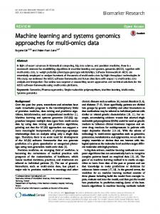
For experimentally testing and validating all the proposed controllers, we use a recently developed modular continuum manipulator designed for showering application (Manti et al., 2016) (Figure 2.2). Since the manipulator is developed for service applications, it is very important that the manipulator is inherently safe while the controller is reasonably accurate. The setup is composed of two hybrid modules, with each module having three pneumatic and three tendon-driven actuators. The McKibben-based flexible fluidic actuators are to be used in tandem with the inelastic cable driven actuators for extension, compression and stiffening. The actuators are supported externally by a flexible helicoidal structure that has been inserted along the entire module thus providing appropriate structural rigidity for our application while maintaining the dexterity of the arm. The unactuated length of the manipulator is 40.5 cm with a diameter of 6 cm. The cables are actuated by six HS-785HB Winch Servo Motors. An electronic proportional micro regulator Series K8P pressure regulator is used for the closed loop control of the chamber pressures. For tracking the position and orientation of the manipulator either the Aurora tracking system (Northern Digital Inc.) with a six DoF electromagnetic probe or the Vicon system is used. The probe is attached at the end of the manipulator. If the environment is free of electromagnetic disturbances, the Aurora system specifies an accuracy of 0.70 mm and 0.30 degrees (RMS). The Aurora system also specifies the uncertainty of each measurement which is useful during the learning step for removing outliers in the data. The Vicon system can reach an accuracy of 0.1mm, however the actual accuracy varies on the size and location of markers, camera and the calibration accuracy.

Chapter 2. Preliminaries

Figure 2.2: (a) The soft manipulator used for the experiments. (b) CAD model of the design.

7

8

Chapter 3

Kinematics Most robotic applications rely on task space controllers. The primary objective of such controllers is to guide the end-effector trajectory, in case of manipulators, or the center of mass trajectory for legged locomotion. However, since these controllers can only act directly on the actuator space, a causal mapping between the task space and actuator space is required. Inverse kinematic mappings are used to derive the configuration space coordinates given the task space coordinates. Inverse kinematic models have been extensively studied for rigid bodied robots by using analytical and machine learning methods. Soft robots present a formidable challenge to modelling due to their high dimensionality. Nonetheless, tractable kinematic models can be developed by adopting a steady-state assumption; i.e. under force equilibrium, the full configuration of the soft manipulator can be defined by a low dimensional state space representation (George Thuruthel et al., 2018). Throughout this thesis, we interchangeably use the term ‘statics’ and ‘kinematics’ even though this is not a common practice in traditional robotics.

3.1 3.1.1

Related Works Model-based approaches

The simplest and most commonly used kinematic/steady-state model assumes that the configuration space of a three dimensional soft module can be parametrized by three variables, more commonly referred to as the constant curvature (CC) approximation (Hannan and Walker, 2003). It reduces an infinite dimensional structure into just three dimensions, thereby ignoring a large portion of the manipulator dynamics. This has been found to be a very good approximation if: (i) the manipulator is uniform in shape and symmetric in actuation design, (ii) external loading effects are negligible, (iii) and torsional effects are minimal. It is important to realize that the CC model arises due to a constant strain approximation along the length of the manipulator and therefore is a model truly valid only in the steady-state condition (Gravagne, Rahn, and Walker, 2003). Gravagne and Walker, 2002a demonstrated that the variations in the kinematic manipulability ellipsoid is much less when going from a low dimension to a high dimension representation of the manipulator configuration. This could explain the relative success of the CC model. For multi-section continuum/soft manipulators, each constant curvature section can be stitched together to provide the Piecewise Constant Curvature (PCC) model (Jones and Walker, 2006a). Concurrently, more complex modelling approach was pursued using beam theory (Gravagne, Rahn, and Walker, 2003) and cosserat rod theory (Trivedi, Lotfi, and Rahn, 2008). However, the improvement in accuracy attained by this increased

Chapter 3. Kinematics

9

complexity was not significant compared to their computation and estimation costs and therefore their usage has been limited. Once a kinematic model is established, it is necessary to invert the kinematics to obtain the desired actuator or configuration space variables. This can be pretty straightforward and has been widely studied for rigid manipulators and can be done with differential inverse kinematics (Bailly and Amirat, 2005), by direct inversion (Camarillo, Carlson, and Salisbury, 2009a) or by optimization (Camarillo, Carlson, and Salisbury, 2009b). Further, a low level controller takes care of tracking in the actuator/joint space, usually using a simple linear closed loop controller. Additionally, actuator compensation techniques might have to be used because of the presence of friction, hysteresis (Xu and Simaan, 2006) or tendon coupling (Jones and Walker, 2006b) that can cause deviations from the forward steady-state model. The need to model and compensate for slackening, tendon load coupling and tendon path coupling for multi-section manipulators was first addressed by Camarillo, Carlson, and Salisbury, 2009a. A numerically estimated static model was used for the forward model and the inverse model was obtained by optimization. However, there still lacked an expression for friction effects and the approach was used only for configuration tracking. One of the fundamental modelling difficulties involved with cable driven actuators is the path coupling among sections. For independent actuation methods, only the load coupling needs to be considered. Further on researchers started investigating the importance of sensors for compensating modeling uncertainties without the necessity for formulating very complex compensation techniques (Bajo, Goldman, and Simaan, 2011). As an extension of (Camarillo, Carlson, and Salisbury, 2009a), a closed loop task space controller was proposed and experimentally validated for the first time in (Camarillo, Carlson, and Salisbury, 2009b) with a 5 DoF per section kinematic model. For this, the inverse kinematics (IK) problem is formulated as a constrained nonlinear optimization problem where the desired joint configuration that reduces the current tracking error is estimated while satisfying the forward kinematic model and cable tension constraints (to avoid slacking). By representing the kinematics in the velocity level, their approach gains leverage in terms of higher accuracy and robustness to model uncertainties, but would need to solve a high level path planner (Refer Figure 3.1). The downside of the direct task space controller is instability (can be solved by lower control frequency; 4Hz for Camarillo, Carlson, and Salisbury, 2009b) and slower convergence. In Bajo, Goldman, and Simaan, 2011, a configuration space controller is proposed which uses external sensory information about the configuration and internal sensory information about the joint variables to achieve asymptotic tracking of a stationary configuration target. By providing additional tracking information and framing a cascaded controller they were able to reduce coupling effects and decrease the phase lag while tracking a time varying trajectory. Being a configuration space feedback controller, the control loop was run faster at 150 Hz. Interestingly, significant phase lag was observed even for tasks at 2 Hz and this is highly undesirable at the low level. Similarly in Penning et al., 2012, two closed loop controllers in the task space (Figure 3.2) and joint space (Figure 3.3) were compared. The advantage of a direct closed loop task space controller is that it can provide asymptotic convergence of the error even with model uncertainties. On the other hand, a joint space controller can offer independent control of the joint variables, allowing for individual tuning and hence more stability, especially if the joint/actuator motions are discrete. Note that for all the above mentioned controllers there is also a closed loop actuator space controller, usually a servo controller, which is assumed to provide perfect tracking. All these methods rely on the


10

CC approximation for modelling.

Figure 3.1: A closed loop task space controller implementation. A∗ represents the desired variable value, Ac represents the commanded variable value

Figure 3.2: A closed loop task space controller implementation.

Figure 3.3: A task space controller implemented by closed loop control in the joint space. Ae represents the variable estimate.

Following the strong coupling between continuum manipulator’s kinematics and static force model, controllers foraying into compliance/force control started to emerge (Mahvash and Dupont, 2011; Goldman, Bajo, and Simaan, 2011; Bajo and Simaan, 2016). In Goldman, Bajo, and Simaan, 2011 it was demonstrated that by knowing the current internal actuation forces and the configuration space variables an estimate of the external generalized forces can be formed. Using the estimate of the external force and the compliance matrix (maps the change in actuator forces to the tip wrenches) a configuration space controller for reducing tip forces for surgical purposes was proposed. As an extension of Goldman, Bajo, and Simaan, 2011, a hybrid position/force controller in the configuration space was realized in Bajo and Simaan, 2016 (Figure 3.4). Desired twist and wrench vectors are projected orthogonally (for decoupling the control effort into feasible motions) and transformed to configuration space references using differential inverse kinematics and the configuration space compliance matrix (maps the change in configuration space variables to the tip wrenches) respectively. Hybrid position/force control was realized in Mahvash and Dupont, 2011 without the need of force sensors. This was done by numerically calculating the transformation matrix that maps the transformation from the tip of an unloaded continuum manipulator to the tip position when acted on by external forces using cosserat rod theory. With the transformation formulation, the desired joint position that attains a particular end effector force and orientation was estimated using fixed point iteration. Compensating model-deviations due to friction and other nonlinear material behavior remains an open research topic.


11

Figure 3.4: Closed loop tasks space control of position and force implementation. Av represents the first order derivative of the variable.

Further on, researchers started to focus on more complex kinematic formulations by extending the CC model, mostly due to the rise of biologically-similar tapering continuum robots. The first such method was the use of the Variable Constant Curvature (VCC) approximation which models a single module as n segments of constant curvature; where the curvature of each segment depends on the radius of the segment, thus creating a high dimensional configuration space (Wang et al., 2013; Mahl, Hildebrandt, and Sawodny, 2014; Mahl et al., 2013). The VCC model for a three section pneumatically actuated continuum robot, with the procedure for segmentation of the sections, was first elucidated in Mahl, Hildebrandt, and Sawodny, 2014; Mahl et al., 2013. A resolved motion rate algorithm was used for the closed loop control of the robot due to the double advantage of redundancy resolution and the robustness it provides to model uncertainties (Figure 3.5). Visual servo control of a two dimensional image feature point in three dimensional space using a cable driven soft conical manipulator was proposed using the VCC model in Wang et al., 2013. A differential kinematics based controller, similar to the one in Mahl, Hildebrandt, and Sawodny, 2014, with the control objective of reducing the feature point tracking error was proposed. An adaptive algorithm for depth estimation was also described. Similarly, efficient numerical techniques for solving in real time the complex cosserat models were detailed in Till et al., 2015, however no control experiments were demonstrated.

Figure 3.5: First order resolved motion rate algorithm for closed loop task space control. Note the similarity to the first implementation in Figure 3.1. The additional feedforward component allows for faster convergence.

Contrary to ongoing developments, use of simplified kinematic models for control was proposed in (Boushaki, Liu, and Poignet, 2014). The idea behind this is that the reduced accuracy due to the inaccurate kinematics can be compensated or even improved with the increased control cycle frequency gained due to the low computational cost. However, the method was validated only on simulations and would not be directly transferable to a real setup at the same frequency without considering the low level dynamics as observed in Bajo, Goldman, and Simaan, 2011. On


12

the other spectrum, a numerically exact approach for statics modelling using asynchronous Finite Element Analysis (FEM) was described in Largilliere et al., 2015. Optimization using quadratic programming (QP) algorithm was used to obtain the inverse solution which is used to control the actuators at high frequencies while a low frequency loop FEM simulation feeds the inputs to the QP solver. Recent developments in terms of model based static controllers are factored on the design aspects. A closed loop task space controller was applied on an interleaved continuumrigid manipulator in Conrad and Zinn, 2015. The main idea of the approach is to use the well behaved rigid links in tandem with the flexible elements to compensate for the errors obtained while tracking a desired tip position thereby obtaining much lower bound on the tracking error. However, the scalability of such designs for high dimensional systems is still a question mark. Currently the manipulator is designed with the rigid components set up at the base, but it will be tricky to add further components in serial. On the other hand, kinematic control of a pneumatically actuated soft manipulator entirely made from a low durometer elastomer was detailed in Marchese and Rus, 2016. The control architecture is similar to Bajo, Goldman, and Simaan, 2011 and tries to achieve tracking of configuration space variables using a cascaded PI-PID in the configuration space and actuator space (cylinder displacement, in this case) respectively. The task space to configuration space inverse kinematics is obtained by solving a nonlinear constrained optimization. Both the above mentioned approaches used the CC approximation for the configuration space model. Model-based static controllers are currently the most widely used and studied strategy for control of continuum/soft robots. A majority of the model-based controllers relies on the CC approximation since more complex models are computationally expensive and are design specific. However, with validation of the CC model for a completely soft robot Marchese and Rus, 2016 and its wide application for control of many continuum/soft robots it is still one of the most reliable and easily applicable method for static control of uniform, low mass manipulators. More complex methodologies have not achieved exceptional performance improvements because of their computational cost and numerous parameters that have to be estimated. This was also observed in recent comparisons among various modelling approaches on the same platform (Sadati et al., 2017). In light of this, model-free approaches provide an alternative means to develop more complex yet accurate, design specific models without any prior knowledge about the underlying structure. In terms of operating space, a closed loop configuration space controller or joint space controller would provide more stable and faster controllers, however cannot guarantee task space error convergence (Unless there is a perfect forward model available). Closed loop task space controllers can theoretically provide the best accuracy. In terms of actuation, tendon driven systems are more difficult to model, whereas pneumatic manipulators would need more sensors.

3.1.2

Model-free approaches

Model-free approaches for control of continuum/soft robots is a relatively new field and offers a wide range of possibilities. Although, these data dependent methods have been used effectively in the field of rigid manipulators (Nguyen-Tuong and Peters, 2011), the same cannot be said for continuum manipulators even though model-free approaches intuitively should fare better in this case. The first usage of a model-free approach for development of a static controller was proposed in


13

Giorelli et al., 2013. The approach was a straightforward direct learning of the inverse statics of a non-redundant (with respect to the actuator space and task space) soft robot using a neural network. Although the method was correctly able to predict the reference cable tensions for reaching a target in the task space in simulations, the approach cannot be scaled for redundant systems and does not consider the stochastic nature of real soft robots. An experimental validation of the same approach was done in Giorelli et al., 2015b for a two DoF and a three DoF (Giorelli et al., 2015a) cable driven soft manipulator and compared with an IK model derived from a numerically exact model. Interestingly, the simple neural network based approach performed significantly better than the computational complex analytical method. The final controller is similar to the diagram shown in Figure 3.6 without the feedback component.

Figure 3.6: A general model free closed loop task space controller implementation. Am represents an auxiliary variable.

An efficient exploration algorithm for generating samples for IK learning was proposed in Rolf and Steil, 2014. The main idea is to use goal babbling to generate samples from the task space to actuator space for high dimensional redundant systems. Since the exploration is goal oriented, it can allow for efficient exploration (by avoiding revisiting an explored task space/actuator space region) and in selecting a desired redundancy resolution scheme. Finally, self-organizing maps are used to learn the IK mapping with generated samples. A feedback scheme for reducing tracking error due to the stochasticity of the model is implemented by virtually shifting the target positions proportional to the error in tracking to generate modified reference positions (Figure 3.6). A highly robust, accurate and generic approach for closed loop task space control of continuum robots was proposed in Yip and Camarillo, 2014 (Figure 3.7). The paper proposes a control strategy based on empirical estimation of the kinematic Jacobian matrix online by incrementally moving each actuator. Optimization is done to minimize the control effort and to keep the cables taut. There is no internal model used for control and therefore the authors have called the approach a ‘model-less’ technique. Although such a strategy solves a lot of difficulties in the control of continuum robots, even allowing manipulation in an unstructured environment, the very low control frequency is of practical concern. The same principal was extended for hybrid force/position control in Yip and Camarillo, 2016, where the stiffness matrix is also computed empirically. Similar to other hybrid force/position controllers, the reference position and forces are projected orthogonally when the manipulator is in contact. Recent model-free approaches have mostly focused on learning the IK representation of continuum robots. In Melingui et al., 2014, an approach for learning the direct mapping between task space and joint space (potentiometer voltage, in this case) is proposed. This involves learning the forward kinematic model first using a neural network and then inverting this learned network using Distal Supervised


14

Figure 3.7: Model-less control strategy.

Learning. However, this approach did not consider the stochasticity of the manipulator and did not implement a feedback error correction scheme. As an improvement of the previous work, in Melingui et al., 2015, the authors try to address the stochasticity of the mapping between the joint space (potentiometer values) and actuator space (chamber pressures) by developing an adaptive sub-controller. This is because for the case of tendon-driven actuation, the actuator space and joint space are linearly related, whereas, for pneumatic actuation an additional non-linear mapping between the actuator space and the joint space must also be considered. The sub-controller comprises of a Modified Elman Neural Network which emulates the actuator kinematics and a Multilayer Perceptron controller that learns to control the actuator variables accordingly. However, the kinematic mapping between the joint space and task space is considered to be non-stochastic which is not necessarily the case. Another technique for learning the IK is proposed in this thesis, where the IK problem is formulated like a differential IK problem using local mappings. This allowed for redundancy resolution as well as reducing stochastic effects. The approach was validated by simulations on a continuum (Thuruthel et al., 2016b) and soft arm (Thuruthel et al., 2016a). Another advantage of such an approach is that it allows multiple solutions to the IK problem globally and can work even if some of the actuators are nonfunctional after the learning process. An extension of the modelling method strengthened with a feedback controller was also experimentally validated (George Thuruthel et al., 2017). It was also observed that even with a simple feedback controller, intelligent behaviors can be obtained in an unstructured environment. An attempt towards transfer learning has also been made, however, limited to simulation (Malekzadeh et al., 2014). The authors develop an algorithm to transfer the reaching skills from a simulated non-CC octopus arm to a simulated CC soft robotic manipulator. The idea is to design dynamic motion primitives through a weighted combination of Gaussian functions representing the joint distribution of the data. This is combined with a statistical regression approach making it robust to external perturbations in the environment. Although this approach seems promising, it requires more experimental work to demonstrate its potential. In a recent work (Ansari et al., 2018), the authors optimize multiple objectives within a reinforcement learning architecture to learn deterministic stationary policies for a soft robot arm module. Although it works in high-dimensions, it is sensitive to external disturbances. An attempt towards fuzzy logic based controllers was shown in (Qi et al., 2016). The idea was to develop numerical estimates of the kinematic Jacobian using prior knowledge based local approximations and interpolation functions. This allows for faster computation, but the advantage of such a method over data driven machine learning approaches is not apparent. Finally, hybrid controller combining both model based and model free approach was proposed in (Lakhal,


15

Melingui, and Merzouki, 2016; Jiang et al., 2017; Reinhart, Shareef, and Steil, 2017). In Lakhal, Melingui, and Merzouki, 2016, the manipulator is modelled as multiple sections with one translational and two rotational degrees of freedom. Then, multiple neural networks are used to resolve redundancy and to obtain the mapping from the task space to the high dimension configuration space. The configuration space to actuator space mapping is done analytically as it was found to be more straightforward. A noticeable limitation of such a method is the high sensory information required, which in the paper, the authors have synthesized from certain empirical data. A polar method was adopted in Jiang et al., 2017, with the configuration space to task space mapping being analytically modelled using the PCC approximation. The actuator space to configuration space mapping is learned also considering possible first order viscoelastic effects. A feedback strategy like in Rolf and Steil, 2014 was also employed to provide high tracking accuracy however only for a planar manipulator. In Reinhart, Shareef, and Steil, 2017, it was shown that by learning only the model error incurred by an analytical model (a CC model), better forward and inverse kinematic models could be obtained. In this way it is also possible to leverage the advantages of an analytical model (like null space motions) along with the generality of learning methods. One of the primary advantages of model-free approaches is to circumvent the need to define the parameters of the configuration space and/or joint space and is independent of the manipulator shape. Due to this, arbitrarily complex kinematic models can be developed depending upon the abundance of the sample data and sensory noise. This is probably why model-free approaches have fared better for systems that are highly nonlinear, non-uniform (Giorelli et al., 2015b), influenced by gravity (Rolf and Steil, 2014; George Thuruthel et al., 2017), or act within unstructured environments where modelling is almost impossible (Yip and Camarillo, 2014). However, for well-behaved compact manipulators in known environments, model-based controllers are still more accurate and reliable. Furthermore, due to their black box nature, stability analysis and convergence proofs are difficult to establish. Static/kinematic controllers assume little or no dynamic coupling between sections. As mentioned in the beginning, static/kinematic controllers rely on the steady state assumption, which hinders accurate and fast motion of soft manipulators. Hence, controllers that consider the dynamic behavior of these manipulators are important for faster, dexterous, efficient, smoother tracking and in situations where coupling effects cannot be ignored.

3.2

Our Solution

As with their rigid counterparts, learning the inverse kinematics model of soft bodies offers two major problems: First, the inverse kinematic/statics solution is not unique and the solution set forms a non-convex set (D’Souza, Vijayakumar, and Schaal, 2001). Furthermore, analytical or numerical methods are difficult to develop and can be computationally expensive. Our objective is to develop kinematic controllers by developing models for the IK solutions of the continuum robot. The forward kinematics can be represented as a mapping between the actuator space (encoder value/length of cables, cable tension, pneumatic pressure, etc.), q , to the end-effector coordinates, x . Assuming that there are no environmental constraints, the forward kinematics can be represented by:


16

x = f (q )

(3.1)

Where, x ∈ Rm is the position and orientation vector; q ∈ Rn is the vector containing the actuator variables; and f is some surjective function. The inverse kinematic model is a mapping between the end-effector coordinates to the actuator variables. Direct inversion of the forward function is not possible when m < n , i.e. when the manipulator is redundant and the solution set of all possible solutions do not form a convex set. To simplify the inversion problem, the forward kinematics can be linearized at a point (qo ), thereby obtaining the formulation; x˙ = J (qo )q˙

(3.2)

Here, J is the Jacobian matrix that transforms actuator velocities, q˙ to end-effector velocities, x. ˙ As was shown by D’Souza, Vijayakumar, and Schaal, 2001, by spatially localizing the actuator variable q, we can ensure convexity of the different IK problem and thereby making the learning problem tractable. By sacrificing slightly on the accuracy, the differential kinematics can be approximated as : ∆x ≈ J (qo )∆q

(3.3)

J ( qi ) qi + 1 ≈ x i + 1 − f ( qi ) + J ( qi ) qi

(3.4)

Where, qi +1 is the actuator configuration that archives the end-effector position xi +1 , while qi is the current actuator configuration. This not only allows us to learn the Inverse Kinematics on a position level but also facilitates spatially localizing q by the sampling method rather than the learning architecture. The spatial localization can be done by ensuring that | qi +1 − qi | is bounded. Note that this will indirectly constrain the end-effector motion spatially. From empirical data, it is recommended that: | qi +1 − qi |< , where is between 3 − 10% of the actuator range. For faster exploration, higher is better, however a lower value provides better accuracy. Much lower values of can theoretically provide better accuracy, but, in reality environmental noise will overpower the information present in the data. The exploration strategy for collecting sample data is done by continuous motor babbling (random actuator motion) whilst ensuring the spatial locality of the actuator variable. Now we can employ any universal function approximator to learn directly the mapping: (xi +1 , qi ) → qi +1 . In our case we are using a single hiddenlayer Multi-Layer Perceptron for this purpose. We are using tan-sigmoid transfer function in the hidden layer and a linear transfer function in the output layer. Since the data is naturally bounded by the actuator range and due to the tan-sigmoid transfer function and learning algorithm, the learned network will always output a valid joint configuration thus ensuring valid motions. Now an important concern is what the response of the learned network would be when the target positions xi +1 cannot be achieved from the current joint configuration by a local motion (Since, the network is trained with data that are obtained by local motions only). One can expect the learned network to be similar to the form given below: qi +1 = G [xi +1 − f (qi ) + Jqi ]

(3.5)

Where, G, is a generalized inverse of J (qi ). When the target inputted is not a local point, the network response just gets scaled as one would expect from equation 3.5, thereby bringing the end-effector position closer to the target. Repeating


17

the algorithm eventually leads to the network converging near the target position. Since neural networks have the ability to generalize well, global learning of the IK can be done without exploring the complete actuator space. This is also aided by the fact that there is always high correlation between local Jacobians. But, it is important that the exploration process obtains data from the boundaries of task space for maximal utilization of the workspace. Simple controllers which learn the mapping (xi +1 , qi ) → qi +1 will fail in the presence of environmental constraints, because for continuum robots, the forward kinematic model is also dependent on the environment. This is due to the numerous underactuated and compliant joints present in a continuum robot. It is a hard task to model all the contacts and get the subsequent kinematic model. Therefore, we propose a simpler way to incorporate feedback correction of errors occurring due to unstructured environmental factors and showcase that this simple strategy can perform well even without any modification of the learned network. Consider a controller which learns the mapping regulated by a different formulation of equation 3.5 shown below: qi + 1 = G [ x i + 1 − x i ] + qi

(3.6)

We can expect a network which learns the mapping: (xi +1 , qi , xi ) → qi +1 to always move along the direction of the Jacobian scaled by the error in tracking: [xi +1 − xi ]. For the case of rigid robots, the information obtained from the endeffector position xi is redundant, however, that is not the case for continuum robots. As the estimate of the Jacobian by the learned network is based only on the current joint configuration it will not be same as the actual Jacobian. However, we argue that even this inaccurate estimate of the Jacobian is enough to force the motion of the end-effector in following a path of minimum possible error under external constraints. In other words, we claim that in the presence of obstacles a decent strategy is to try to reach the target towards the current estimate of the Jacobian and the high dimensionality and compliance of the body will guide the manipulator in the best path; as long as the controller tries to reduce the tracking error with the current estimate of the Jacobian. In addition, adding the end effector position as an input makes the learning more tolerant to noise incurred due to the stochasticity of the system, which greatly improves the learning process.

3.3 3.3.1

Simulation Results Open-Loop Kinematic Controller

On the Bionic Handling Assistant(BHA) The training data is obtained from a kinematic model of the BHA (Rolf and Steil, 2012). The model uses a constant curvature approximation for modelling the continuum kinematics of the manipulator. The robot is composed of three segments; each segment is actuated by the three pneumatic actuators. The kinematic model takes in as input the length of each actuator and outputs the three dimensional coordinates of the end-effector with respect to a reference frame fixed at the origin. Figure 3.8a shows the schematic of the BHA. The model is a very good representation of the real BHA with a relative error of 1%.


18

Figure 3.8: a Fifty randomly selected target points and their IK solutions, b Error values for each target point with their steps for convergence, c Trajectory tracking experiment and results, d Error values with mean and standard deviation for each rotation (100 steps), e Trajectory tracking experiment with last three joints fixed, f Error values with mean and standard deviation for each rotation (100 steps)

Three types of experiments are conducted on the learned open-loop IK model to validate and analyze the proposed approach. The first one is a simple ‘reaching a point’ simulation. Fifty points are randomly chosen (Figure 3.8a) and the IK solver gives its estimate of the joint configurations. The forward model is used to compare the desired positions and the IK estimates. The errors along with the mean and standard deviation are shown in Figure 3.8b. Since the points are not near to the starting point, the solver takes an average of 5.68 steps to converge to a value within a range of 1mm with a standard deviation of 1.504mm. The second experiment is a circular trajectory tracking simulation. The target


19

trajectory is a circle centered at [0, 0, 0.7m] with a radius of 0.2 meters and the endeffector starting at the home position [0, 0, 0.9m]. The same path is followed twice. The path is discretized into 200 individual points, 100 points for one rotation. Figure 3.8c shows a comparison of the path derived from the IK solver with the target path. Figure 3.8d shows the magnitude of error in following the path along with the mean and standard deviation for each rotation. The large error in the beginning is because the manipulator starts from the home position which is away from the target path. The final simulation has the same circular target trajectory, but with the last three joints locked at a fixed value. The IK solver is given no knowledge about the freezing of the three joints. Therefore, the IK solver still outputs the next configuration for all the joints in each iteration, however, only the first six joints will be modified accordingly and the last three joints will maintain their initial configuration. The trajectory followed in this new setting is shown in Figure 3.8e. The corresponding absolute errors with mean and standard deviation for each rotation are shown in Figure 3.8f. Note that for the last two experiments only one step is needed to get the appropriate IK solution as the target points are nearby. The results show that solutions provided by the IK solver are still good despite losing three degrees of actuation. This shows that the IK solver is able to provide a meaningful solution at any joint configuration. However, note that this is only possible because of the redundancy present in the system. Interestingly, this means that we could exploit the redundancy of the system for executing secondary tasks, by compromising correspondingly on the primary task. On a Steady State Model of an Octopus inspired manipulator For testing the steady state controller, we have used a steady state model of a tendon driven soft continuum robot (Renda et al., 2012). The sample data for learning the inverse static (IS) model is obtained from this steady state model. The orientation data is also recorded and learned. The soft continuum robot is modelled as a cosserat beam. A cosserat beam can be visualized as a continuum body which is composed of infinitesimally small rigid bodies that can rotate independently from the neighbouring element. We are ignoring the effects of shear stresses in our formulation (Euler-Bernoulli hypothesis). This restricts the DoF of each element to four. The total length of our manipulator is 31 centimetres, divided into a section per centimetre. There are three anchorage planes along the length of the manipulator. Each anchorage plane has four cables attached to it; each spaced apart by an angle of 90 degrees. Figure 3.9 shows the reachable workspace of the robot obtained by random exploration in the actuator space.


Figure 3.9:

20

Schematic of the simulated manipulator and its workspace

The main advantage of the proposed method is its ability to provide global solutions to the IS problem without the need to plan a path from the starting point. So, the first tests were to evaluate if the IS solver can provide accurate actuator configuration for random target points in the workspace. Fifty points (x∈(-0.05,0.35), y∈(-0.25,0.25), z∈(-0.2,0.2)) were randomly selected from the sample data along with their corresponding orientation. Since the target points are not close to the home position (0.31[m], 0[m], 0[m]), the solver needs more than one iteration for converging to the right solution. Figure 3.10 shows the test results for this experiment. The proposed method is able to generate results with a mean positional error of 0.012 meters and mean orientation error of 7.4 degrees. The method converges with an average of 3.56 steps for convergence within a range of 1mm. The same fifty target points were again used in the IS solver for a starting point at one of the extreme boundary points (-0.02m,-0.16m,-0.01m). The corresponding results are shown in Figure 3.11. The average errors increase in this case. The average positional error goes to 0.015 meters and the average orientation error goes to 9.92 degrees. The convergence speed remains the same with each target taking an average of 3.68 iterations for convergence. Note that even though the magnitude of error increases, the error pattern remains relatively similar. We suggest that these points are under-represented in the sample data and therefore the learning system does not have an adequate representation around that region. One possible work-around is to develop algorithms that perform motor babbling initially and then later switch to a more goal oriented exploration strategy.


21

Figure 3.10: Simulation results for the fifty points experiment at the natural starting point. The thick lines represent the mean of the data and the dotted lines on either side of the mean represent the standard deviation.

Figure 3.11: Simulation results for the fifty points experiment for a starting point at one of the boundary extrema.

The next set of simulations were conducted for continuous targets, i.e. the target points are locally adjacent and therefore form a continuous path. As the target points are close by, the IS solver can output a solution in one iteration. Two such paths were used for evaluation. The first one is a circular path of radius 0.1 meters, centered at (0.25[m], 0[m], 0[m]), with a fixed orientation parallel to the X axis (Figure 3.12). The other path is a fixed point with a continuous change in elevation (0→90→0 degrees) and azimuth (0→180 degrees). Figure 3.13 shows the target orientation vectors for this simulation and the corresponding solutions from the IS solver. For both tests, the manipulator starts from the home position (Zero force position). The results of both tests are shown in Table 1.


22

Figure 3.12: Continuous positional path following with fixed orientation. The target orientation is a vector perpendicular to the YZ plane

Figure 3.13: Continuous angular path following.

Table 3.1: Continuous path results.

Test Circular Path Angular Path

3.3.2

Position Error (Mean ± S.D.)[m] 0.0085 ± 0.0028 0.0118 ± 0.0059

Orientation Error (Mean ± S.D.)[degrees] 7.33 ± 3.98 3.21 ± 1.71

Closed-Loop Kinematic Controller

In this section the results of two simulation experiments performed to test and validate the scheme for integrating the end-effector feedback to the learning scheme are described. Through these simulations we try to demonstrate that the proposed controller can accommodate changes in kinematics of the robot without retraining the network. The simulations are conducted on a kinematic model of the same bionic handling assistant. The continuum kinematics is modelled by a constant curvature approximation and the manipulator has nine DoFs.


23

To begin with data samples are generated by continuous motor babbling as mentioned in the previous section and the mapping (xi +1 , qi , xi ) → qi +1 is learned. During the learning phase, no external disturbances are applied to the system and therefore information about the current end-effector position (xi ) is actually redundant. Our interest lies in studying the effects of external factors on the manipulator and the subsequent response of the learned system. Since the simulation model is purely kinematic, it is not possible to apply external forces directly. Therefore the only way to model external factors is to modify the forward kinematics of the model itself. Firstly, we set an offset to the end-effector position outputted by the simulator and observe the performance of the solver. This is equivalent to adding a constant value to the forward kinematic model. Note that the offset is added after learning and the IK solver does not have any information about the offset other than what is observed from the end-effector position. The target position is fixed in all cases. Therefore, the solver has to output different actuator configurations for reaching the same target because of the offset. Figure 3.14 shows the error in tracking by the solver with the change in offset value added in the X direction. value is shown in percentage of the actuator range to showcase its effect on efficient learning. The number of samples collected is the same for all experiments. We can observe that for optimum value of , the error in tracking can be reduced by the proposed feedback scheme. If there were to be no end-effector feedback in the IK solver, the tracking error will be directly proportional to the offset distance as the end-effector will always go the same actuator configuration, since the inputs (target) remain the same. Furthermore, we can realize more nonlinear variations in the forward model by modifying the cable lengths after learning the IK model. Figure 3.15 shows the performance of the IK solver with end-effector feedback and the IK solver without feedback when the initial length of one of the nine cables is reduced. For more clarity, if the current cable length is qo , the modified forward model always calculates the end effector position with the new cable length qo − K(K is a constant and denoted with respect to the initial cable length in Figure 3.15), while for the learned IK solver, the input still remains as qo . For the case of the IK solver with end-effector feedback, the position of the end-effector along with the information learned from the initial kinematic model is enough for accurate tracking of the target. It must be brought to the attention of the reader that network is never explicitly directed to reduce the tracking error; the underlying error correction system is arising purely from the data and the learning formulation.


24

Figure 3.14: Performance of the closed loop kinematic controller with offset added to kinematic model for different values of . The target is a fixed point for all cases.

Figure 3.15: Comparison of the performance of the closed loop kinematic controller and the open loop kinematic controller with nonlinear changes in the forward kinematics. The target is a fixed point for all cases.

3.4

Experimental Results

In order to test and validate the performance of the solver four sets of experiments are conducted for real-time kinematic control of the manipulator with the learned closed-loop IK solver. The experiments are conducted for evaluating the performance of the solver for global point to point motion, local path following, local path following in an unstructured environment and disturbance rejection while maintaining a particular position. For all the experiments the manipulator starts from the home position, which is the configuration with all the actuators at the zero position. Figure 3.16 shows an overview of the IK solver based control system. The weights of the neural network are also not updated during any of the experiments.


25

Figure 3.16: Overview of the closed loop kinematic controller.

3.4.1

Point to Point motion for pose control

For the first experiment, twenty-five random points are selected from the manipulator workspace and the manipulator is commanded to reach each pose in succession using the solution provided by the IK solver. The points are selected from the workspace to ensure that the target is reachable as it is difficult to know beforehand whether a particular position and orientation is reachable. Since the targets are not local points, the solver will require few steps to converge. This makes the solutions fundamentally different from the training outputs and dependent on the initial conditions. Therefore it is possible to obtain multiple solutions for the same target in case the manipulator is redundant for that case. The IK solver converges near the target within ten steps for all the targets. There is a delay of 1sec between each step, during execution to ensure that the static state is reached. Table 3.2 shows the average and standard deviations of the absolute errors incurred while tracking the targets. Table 3.2: Point to Point Motion Performance.

Position (mm) X (mm) Y (mm) Z (mm) Yaw (degrees) Pitch (degrees) Roll (degrees)

3.4.2

Mean Error 9.67 5.53 5.04 4.03 2.76 1.84 3.85

Standard Deviation 5.33 4.08 4.59 3.56 5.42 1.83 7.02

Trajectory following with IK solver for position and pose

The next experiment is to test the performance of the solver in following a continuous path in the task space. Although the targets are local points, the difficulty lies in the fact that the corresponding actuator configurations need not be continuous in the actuator space. There are two trials conducted for this experiment. The first trial is conducted with the IK solver for position with the target path being a straight line of length 20 centimeters from starting to end divided into 40 waypoints. The IK solver is given only one step to provide the solution for each waypoint with each step given 1 sec to settle. The second trial is conducted with the IK solver for pose with the same target positions and a fixed orientation of [90, 0, 180]. Figure 3.17 shows the errors in position and Figure 3.18,3.19 shows the errors in orientation of the manipulator in following the trajectory. The tracking difference shown in Figure 3.18 is just for comparison purpose with the controller for pose. The average positional


26

error for line following using the kinematic controller for position is 23mm and the same for the pose controller is 37mm. Since the target is updated every step, the IK solver would not be able to converge to the best solution for each target and consequently the errors are higher for this experiment. In case of trajectory following with a fixed orientation it must be mentioned that some of the targets are statically unreachable. It is in our interest to analyze the IK solver even if the targets are not reachable.

Figure 3.17: Positional error in tracking for the two kinematic controllers.

Figure 3.18: Orientation error for the position kinematic controller given for evaluating the kinematic controller for pose.

Figure 3.19: Orientation error while tracking using the kinematic controller for pose.


27

Since the IK model is constructed by a neural network, the behaviour of the solver when the target is an outliers (For the case when the target is not reachable) is difficult to be foreseen. The underlying algorithm is majorly dependent on the training data. Figure 3.20a shows the configurations of the manipulator during the path following task using the IK solver for position. Due to the manipulator constraints it is impossible for the IK solver for pose to reach the desired target during the beginning of the task and towards the end. The higher errors in position as shown in Figure 3.17 can be attributed to this. This can be inferred from the workspace of the manipulator obtained during the sampling process. We can see that there is a tradeoff between tracking the position and orientation of the robot. However, presently, it is difficult to quantify how the solver prioritizes for reducing the orientation and position tracking errors or even if there is such a trade-off internally.

Figure 3.20: a)Configuration of the real manipulator at different time steps during the line following task.b) Configuration of the real manipulator for the same corresponding time steps during the line following task in the presence of an obstacle

3.4.3

Trajectory following in an unstructured environment

The next test is to see the effect of an unstructured environment while executing a task. The trajectory is the same straight line position path mentioned in the previous section but with just 20 points instead of 40. Each step is updated at 0.25 sec. This is to ensure that some of the momentum is still conserved between each step. A cylindrical obstacle of diameter 8cm is placed in between the path such that the centre of the cylinder lies around [10cm ,-30 cm] (Figure 3.21). We are only analysing the performance of the IK solver for position as the manipulator is only redundant for this task. Figure 3.20b shows the configurations of the manipulator while performing the task. The numerous DoFs and compliance in the body aid the controller in tracking the best possible path under the circumstances. By a quick comparison with task shown in Figure 3.20a we can see the various kinematic configurations that the manipulator is able to achieve with the help of the environment, which are otherwise unattainable. This is one of the key characteristics of continuum robots. The ability of continuum robots to have modified kinematics in the presence of external forces makes it almost impossible to get accurate formulation of the kinematics, on the contrary, it opens up the possibility of using the environment to guide the manipulator and facilitate the control objective. Through this experiment we demonstrate that approximate IK models with end-effector feedback can work in collaboration with the morphological properties of the robot to accomplish tasks even in an unstructured environment. Also noteworthy is the importance of friction in this task. We noticed that very low friction can lead to slippage and cause the manipulator to overshoot from its desired target. Figure 3.21 shows the top view of the path that


28

the end effector traces in the presence of the obstacle and Figure 3.22 shows the path without the obstacle. The rigidity of the helicoidal structure does prevent the manipulator from fully conforming to the shape of the obstacle and the tracking error experienced due to that is visible towards the end of the path in Figure 3.20a and Figure 3.20b. The forces on the manipulator due to the height of the obstacle also affect the tracking performance.

Figure 3.21: Path of the end-effector in the presence of an obstacle in a line following task.

Figure 3.22: Path of the end-effector in an uninterrupted line following task.

3.4.4

Disturbance rejection during position control

The final test is for showcasing the importance of the end-effector feedback for compensating external disturbances. Under external disturbances, the kinematics of the manipulator will get modified as pointed out in the simulations section. Therefore the IK solver needs to provide new solutions for reaching the same target. For this experiment the external forces are applied by hand after the manipulator has converged to the desired target. Due to the compliance of the body, the manipulator


29

can deform without disturbing the servo position. Consequently, the only change in the input to the IK solver is the change in the end-effector position. We are not concerned with the exact forces or deformations applied to the manipulator as the experiments are aimed to see if the IK solver can output different solutions just by the change in end-effector position and if the solutions can decrease the error in tracking. Clearly there would not be any reaction from an IK solver without the feedback about the end-effector position as the actuator configuration remains the same under the disturbance. Besides that, due to the change in kinematics induced by the disturbance, the new inputs provided to the neural network are outliers when compared to the training data. Thus, it is essential to verify that the network can provide decent solutions and more importantly to see that the network does not get saturated. Figure 3.23 shows the configuration of the manipulator after disturbance and the final configuration derived from the IK solver for 4 different cases. The four trials are conducted in sequence and the solver is updated every 0.5 sec. From the figures we can observe that controller is able to respond exceedingly well to the external disturbances. The error in tracking is reduced even with the change in kinematics and from the images we can observe that the manipulator can reach the same target with different configurations. Again, it must be emphasized that the IK solver is never explicitly commanded to reduce the tracking error and also that the mechanical constraints of the manipulator hamper further reduction of the tracking error. The perceived controller is arising purely from the IK representation and the sample data.


Figure 3.23: Disturbance rejection using the kinematic controller. Four cases are shown in the experiment with configuration of the manipulator after disturbance shown first and the final configuration shown in the end. The complete tracking error is shown below.

30

31

Chapter 4

Dynamics 4.1 4.1.1

Related Work Model-based approaches

Probably the most challenging field in the control of continuum/soft robots is the development of non-static controllers that consider the complete dynamics of the whole manipulator. Development of dynamic controllers would require the formulation of the kinematic model and an associated dynamic formulation. Kinematic models are difficult to develop themselves and a dynamic formulation based on these imprecise models aggravates the model uncertainties (Trivedi, Lotfi, and Rahn, 2007). On the other hand, even if exact kinematic and dynamic models are available, an appropriate controller would then require high dimensional sensory feedback (Renda et al., 2014). Moreover, some dynamic properties/disturbances are inherently uncontrollable due to their under-actuated nature (Gravagne, Rahn, and Walker, 2003). Development of reliable parameter estimation algorithms and accurate sensory information is also crucial. One of the first theoretical studies on the dynamic control of continuum robots was done in Gravagne and Walker, 2002b. In Gravagne and Walker, 2002b, it was validated through simulations of a planar single multi-section continuum robot that a simple feedforward and feedback PD controller can achieve exponential tracking of a set point. The feedforward component inputs the actuator torques that satisfies the static holding torques and the feedback component ensures the convergence of the set point position. A similar experimental study showed that a simple proportional controller can regulate the orientation of a planar continuum robot and a PD controller with coupling compensation can damp out manipulator vibrations (Gravagne, Rahn, and Walker, 2003). Nonetheless, these studies were conducted on simplified models which do not capture the true nonlinearities of continuum/soft robots. The first closed loop task space dynamic controller for continuum robots was demonstrated in Kapadia and Walker, 2011, although, only by simulations. The kinematic for the two dimensional multi-section robot was formulated using the CC model and the corresponding dynamic model in the configuration was presented in the Euler-Lagrangian form using lumped dynamic parameters. One main difference of such a model from the dynamic model of a rigid robot is the addition of the potential energy due to bending and extension (dependent only on the kinematic configuration). In this dynamic equation, the task space state variables can be substituted in place of the configuration state variables using the kinematic model. Note that this way small errors in the kinematic model will exponentially build-up when computing the higher order states and thereby affect the accuracy of dynamic

Chapter 4. Dynamics

32

model. The implemented controller can be described as a PD computed torque controller where the auxiliary control signal is represented in terms of the task space variables. An additional term for controlling the configuration space in the null space is also added. Although the robustness of the controller is shown by adding Gaussian white noise, the performance of such a controller can only be validated experimentally since it hinges on the CC approximation. However, the validity of the CC model for the same model was concurrently questioned in Trivedi, Lotfi, and Rahn, 2007. Furthermore, it must be bought to the attention of the reader that the stability proof was derived assuming that the kinematic and dynamic model is perfect. A different control approach for the same kinematic and dynamic model, in simulation, was done using a sliding mode controller in Kapadia et al., 2010, however, only for closed loop configuration space control. A first order (assuming that the input output relative degree is two) sliding surface is defined as the filtered tracking error for this purpose. The advantage of a sliding mode controller over a simple inverse dynamics based PD controller is the higher robustness to model uncertainties; the downside being the slower error convergence, chattering and higher gain requirements. An experimental evaluation of this method was conducted with a planar three section continuum arm in Kapadia, Fry, and Walker, 2014, along with comparisons to a simple feedback linearization based PD controller in the configuration space. It was observed that the sliding mode controller performed better in terms of accuracy and speed indicating that model uncertainties were significant. Additionally, a task space controller for teleoperation was demonstrated using the controller mentioned in Kapadia and Walker, 2011, which showed good tracking performance for a low frequency reference. Considering the fact that the actuator dynamics of pneumatic actuators are slower and more nonlinear than tendon driven actuators, works focusing on optimal dynamic controllers for pneumatically actuated manipulators started to emerge. One such approach for trajectory optimization was demonstrated using simulations in Falkenhahn, Hildebrandt, and Sawodny, 2014, where the objective was to estimate the optimal trajectory that reduces the transition time and actuator jerk. The nonlinear optimization problem is formulated with kinematic constraints (CC model), actuator dynamic constraints and boundary constraints with the mass flow as the trajectory variable. Along the same lines, a trajectory optimization scheme for a comprehensive dynamic model of a soft planar manipulator was described in Marchese, Tedrake, and Rus, 2016 (Figure 4.1). Using the CC model for expressing the kinematics of the manipulator, a dynamic model was derived in the configuration space. A detailed derivation for calculating the generalized torques from the cylinder displacement and reference input is described in the paper. A direct collocation approach is employed to simultaneously identify the optimal generalized torques and corresponding manipulator state with the systems kinematics, dynamics, boundary conditions and tracking objective as constraints. The objective function is to reduce the final end-effector velocity. An optimization problem is used for obtaining the optimal reference inputs to the actuator to realize the initial trajectory. Another advantage of a solving the control problem as an optimization problem is that it alleviates the need for a high level path planner. The open loop policy was successfully able to reach statically unreachable target points with high probability; the first demonstration in the field of continuum/soft manipulators. Even then an iterative learning control scheme to re-identify the system parameters was required in between trials for best performance.

Chapter 4. Dynamics

33

Figure 4.1: Trajectory optimization algorithm for open loop dynamic task space control.

Another comprehensive model-based controller, seemingly a variation of Kapadia and Walker, 2011, based on the dynamics of the joint space was proposed in Falkenhahn et al., 2015. The kinematics is based on the CC model and the dynamic model is represented in the joint space. A PD computed torque controller in the joint space is proposed. In order to transform the generalized torques used in the dynamic model to the desired actuator pressures’, an inversion scheme is proposed. Experiments even without the PD term showed decent results, validating the dynamic model. An extension of Falkenhahn et al., 2015, which also considers the dynamics of the pneumatic chambers, was proposed in Falkenhahn et al., 2017 (Figure 4.2). With this, an inner loop decoupled PD computed torque controller is cascaded to the existing controller. Consideration of the pneumatic dynamics is important because its response is slower and more nonlinear compared to the dynamics of electromagnetic actuators. Since the controller does not consider the actuator and kinematic constraints, the performance is currently limited.

Figure 4.2: Joint space dynamic controller by feedback linearization.

A recent interesting approach in the field of soft robotic manipulators in terms of design and control was stated in Best et al., 2016. This soft humanoid robot was constructed such that the joints are similar to traditional rotational joints. Therefore, the kinematics of the manipulator can be modeled like traditional rigid robots allowing for much simpler dynamics models, which are identified empirically. The authors have ignored gravitational and cross coupling effects and the relationship between joint torques and pressure is derived. Due to the simplified model and design, a model predictive controller (MPC) in the joint space could be implemented at high frequency (300 Hz). Dynamic controllers are important for industrial applications where time and cost is also important along with the accuracy. Model based dynamic controllers for continuum/soft manipulators are still in their nascent stage, and consequently, there are a multitude of gaps that should be addressed in design, modelling, and control. Dynamic models directly mapping the control inputs (voltage, pressure or encoder values) to the task space variables should provide the ideal performance

Chapter 4. Dynamics

34

for any model based control approach. Currently, most of the dynamic control approaches are focused on the joint space control with an exception of few (Marchese, Tedrake, and Rus, 2016). Even in this case, due to the computational complexity, the controller had to be designed in open-loop for a planar uniform manipulator. However, if the feedforward controller is perfect, this would be the most ideal choice. MPCs are ideal candidates for control of these continuum/soft manipulators, allowing for low gain accurate control. Their application is currently limited only because of the computational complexity of the current dynamic models. With the increase in computational power, sensing capabilities and intelligent controllers, we can expect better developments in model based dynamic controllers. Alternatively, another route to consider is machine learning based approaches, either for learning open loop controllers, for dynamic compensation or for learning black box dynamic models.

4.1.2

Model-free approaches

Model-free approaches for dynamic control of continuum/soft manipulators are still a relatively unexplored area. Nonetheless, the earliest usage of machine learning techniques for control of continuum robots was implemented for compensating for dynamic uncertainties in Braganza et al., 2007 (Figure 4.3). However, the methodology was described only for closed loop dynamic control of the joint variables. The control architecture is composed of a feedback component which is based on a continuous asymptotic tracking control strategy for uncertain nonlinear systems (similar to a second order sliding mode controller) (Xian et al., 2004) and a feedforward component made using neural networks. The objective of the neural network is to compensate for the dynamic uncertainties and thereby reducing the uncertainty bound that improves the performance of the feedback controller.

Figure 4.3: Model-Free dynamic controller in the joint space.

To sum up, although model-free approaches offer a relatively simpler path for developing dynamic controllers, practical applications are limited either due to training time or stability concerns (Venkatraman, Hebert, and Bagnell, 2015). Nonetheless, it is a possibility that should be looked upon, especially with the growth of more robust algorithms for training recurrent dynamic network (Bengio et al., 2015). That being said, hybrid controllers that merge model-based and model-free approaches could also be a viable approach to consider. This chapter presents work on model-free development of dynamic models for dynamic control of soft robotic manipulators. We present the development of a direct direct actuator space to task space dynamic model and its application for openloop dynamic control (Thuruthel et al., 2017a) and behavioral studies on the Octopus Vulgaris. The approach involved learning the forward dynamic model using a class

Chapter 4. Dynamics

35

of recurrent neural network and employing trajectory optimization on the learned model. Such types of controllers reveal a different region of dynamic behavior that a soft manipulator can attain in terms of speed, workspace volume and efficiency. The advantages of a model free approach are clearly evident in terms of the ease of modelling, accuracy and low sensory requirements. Finally, we show how this learned forward dynamic model can be used further to evaluate self stabilizing open-loop trajectories and for closed-loop dynamic control using model-based reinforcement learning.

4.2 4.2.1

Theory Learning the forward dynamic model

In this section we describe how our learned dynamic model is formulated and developed. This learned model will be verified on the simulated model described above and on an real soft robotic platform for validation. Assume that the infinite dimensional configuration space can be approximated using an n-dimensional vector space. The kinematics of the manipulator can now be represented as: x = F (q )

(4.1)

Where, x is the task space (here we are referring to the observable output space) variable and q ∈ Rn is the configuration space variable. In order to obtain this inverse kinematics, a sufficient condition is that the dimension of the task space variable is also n. Consequently all instances of the configuration space variable q can be replaced by the task space variable x. Note that the approximation of the inverse kinematics (consequently the forward dynamics) becomes more accurate with a higher dimensional task space representation. Using these assumptions, it is possible to transform the forward dynamics of the manipulator from the usual form given in 4.2 to a form using only the task space variables as shown in 4.3: M (q )q¨ + V (q )q˙ + P (q ) = τ

(4.2)

¯ (q )q¨ + V¯ (q )q˙ + P¯ (q ) = τ M

(4.3)

Here, τ ∈ Rm are the control inputs. M, V , P represents the inertia matrix, Centripetal - Coriolis forces and potential energy stored due to gravity/deformation ¯ V¯ , P¯ are the corresponding matrices obtained after the transformarespectively. M, tion. This implies that, under these assumptions, it is always possible to learn a direct mapping between the states of the task space variables and the control inputs: (τ, x, x˙ ) → x¨ Consequently, by varying the dimension of the task space (number of sensory inputs), the user can arbitrarily increase or decrease the complexity and accuracy of the dynamic/kinematic model. This is a huge advantage that machine learning provides for learning the dynamics of a soft manipulator. On the contrary, for model-based approaches, the analytical dynamic model determines the sensory requirements (not just the dimensionality but also the type). For instance, models that are based on the CC approximation rely on cable potentiometers for measuring the length of modules (at least in the case of pneumatically actuated manipulators). For rigid robots, the dimension of the joint space (equivalently to the configuration space) is finite and therefore the number of sensors required is fixed.

Chapter 4. Dynamics

36

Taking cue from the previous works on learned kinematic controllers, we modify the mapping in terms of absolute values, there obtaining the new mapping: (τ c , xp , xc ) → xn , where the superscript p represents the previous value of the variable, c represents the current value and n represents the next value. The new mapping is an approximation of the continuous dynamic model using a finite difference approximation. This would restrict the learned dynamic model to have a fixed step size. But by representing the variables only in absolute terms, we gain three main advantages; primarily, such a mapping allows us to represent the dynamic model using a recurrent neural network (see figure 4.4). The advantages of a nonlinear autoregressive network with exogenous inputs (NARX), for long-term time series prediction, have been widely discussed (Menezes Jr and Barreto, 2008; Diaconescu, 2008). Additionally, representing the dynamic model using only absolute terms also helps in encoding the boundary conditions in the data which, in turn, helps in the stability of the network. Finally, in this way we can avoid taking first order and second order derivatives of the position term which would increase the variance of any existing noise. This would further deteriorate the prediction performance. For developing a multi-step prediction model for the forward dynamics we are using a nonlinear autoregressive network with exogenous inputs (NARX). The advantage of using a recurrent-dynamic network over a recursive feedforward-dynamic network is that such networks are more accurate as the training is done to reduce the cumulative error over the whole continuous training set (feedforward networks try to only reduce the prediction error for each step and thereby prone to overfitting and instability). Note that the inputs are normalized inside the network.

Figure 4.4: The architecture of the dynamic model using the NARX network.

The training of the network is done in two steps. Initially, the network is trained in open loop by unfolding the recurrent network and training by Bayesian Regularization. However, this trained network is prone to over fitting and therefore the network is closed and further trained using the same network weights (closing the loop does not change the size of the network). The performance function for the open network is calculated as: MSE =

T 1X kXt − f (Xt−1 , Ut )k2 T t =0

(4.4)

Chapter 4. Dynamics

37

Where, X is the input vector and U is the exogenous input vector. The function f represents the mapping formed by the neural network. For training the recurrent network Levenberg-Marquardt backpropagation is used and a validation set is used to avoid overfitting. Directly training the closed loop network from randomly initialized weights is not desirable as the training would be highly susceptible to the gradient exploding problem. Also, the training and testing sets are divided into continuous (to keep time correlations intact) blocks in the ratio 70:30 for the first step (open loop network) then the training, testing and validation set are divided in the ratio 70:15:15 for the final step (closed loop network). The performance function is now represented as: T 1X ˆ MSE = kXt − f (Xt−1 , Ut )k2 T

(4.5)

t =0

Here, Xˆ t is the prediction of the NARX network in the previous iteration. Now the learning algorithm is not trying to reduce the single-step error, but the whole multi-step prediction error (the performance function is the only difference between the open loop network and the closed loop network).

4.2.2

Trajectory optimization

Once we obtain the learned dynamic model of the manipulator, trajectory optimization can be performed for developing an open loop predictive controller. For this purpose, we are employing a single shooting technique for obtaining the optimal control policies. Let the fixed control horizon be tf , it is discretised by a fixed step size of dt. Given the control policy, the trajectory of the dynamic system can be simulated using the recurrent neural network. xi +1 = f (xi , xi−1 , τi )∀i = 1 . . .

tf

(4.6) dt Where, xi , xi−1 and xi +1 represent the current, previous and next state positions of the manipulator, respectively. τi is the forces applied on all the cables at each time step and f represents the learned mapping. To simplify the optimization problem and for computational reasons we reduce the number of variables by expanding the control frequency to t1 (ts is 50 milliseconds in our case). The control inputs for each s time step dt can now be written as:  t  m  τi−1 mod (i, dts ) , 0 τim ≡  ∀m = 1 . . . M (4.7) ts  τ¯ m )=0 mod (i, dt k t dt $ % t k= ts

i=

∀ t = 0 .. tf ∀ t = 0 .. tf

Here, M is the number of actuators and t is the current time. The time dependent ¯ control policy is represented by the low dimensional vector τ: Π (t ) =τ¯im

∀ m = 1 .. M

(4.8)

The optimal policy can be estimated by minimizing the objective function given below:

Chapter 4. Dynamics

38

 

2 X 



task des T Π (t ) = min 

x tf − x

+ τi R τi  τ ∗

dt

(4.9)

i

t subject to 0 ∀ m = 1 .. M and i = dt The input weighting coefficient R is an identity matrix in our case. The control objective is formulated to reach a desired position at the end of the control horizon while simultaneously optimizing the control effort. No constraint on the final velocity is given since it difficult to estimate if a point is statically and dynamically reachable using only the learned model. For solving this nonlinear optimization problem, we use the iterative sequential quadratic programming (SQP) algorithm (Fletcher, 2013). Since the dynamic model is represented by neural networks with continuous and smooth transfer functions, the objective function is always twice continuously differentiable. The derivatives and double derivatives are estimated by numerical methods for the objective function. MATLAB fmincon function is used for optimization. After optimization we obtain an optimal policy that controls the manipulator to the desired position in the commanded time period. Using parallel processing on 4 cores, a 10 step iteration for a control horizon of 1 second (60 variables) takes 6.2 seconds in average. This is not fast enough for implementing a closed loop Model Predictive controller, therefore the developed controller is fully open loop with no feedback. m ≤τim ≤τmax

4.3

Open-loop dynamic control

The simulation studies are conducted on a simulated cable driven two-section soft manipulator (Renda et al., 2016a). The second section is un-actuated and the first section is actuated by three radially arranged cables. The exploration is done by inputting pseudorandom variable-amplitude square wave sequences, with a 50 percent probability of the actuator being idle. The exploration signals are decided based on empirical data. The maximum force applicable by the cables is fixed to 3 Newtons. Sampling is done at a fixed frequency of 100 Hz and consists of 7000 samples, amounting to a duration of 70 seconds. The corresponding explored workspace is shown in Figure 4.5. Additionally, more goal directed explorations can be performed after learning the forward dynamics with the initial sample, for more efficient and complete exploration.

Chapter 4. Dynamics

39

Figure 4.5: Workspace of the manipulator obtained by the random exploration.

4.3.1

Deciding task space dimension

As previously mentioned, it is up to the user to decide the dimension of the task variables that determines the underlying dynamic model. Clearly, providing more information about the state of the manipulator leads to a better prediction. The mean prediction error for different number of task space parameters is shown in Figure 4.6. The prediction is computed by the recurrent network for the whole sample data by a single multi-step ahead simulation (a 70 seconds simulation). Note that this is only the prediction error of the forward dynamic model. For the three dimensional case, only the Cartesian position of the end-effector is used for prediction. For the six dimensional case two scenarios are compared; the first one uses the Cartesian position of the tip of both sections and the second case uses only Cartesian positions of the tip (end-effector) and the midpoint of the second section. For the twelve dimensional case, Cartesian positions of the tip and the mid-point of each section are used. For all the cases, the network size is fixed (35 neurons).

Figure 4.6: Mean multi-step prediction error using the NARX network for different manipulator characteristics.

Furthermore, we also try to investigate how the prediction accuracy is affected by material properties and force limits (Figure 4.6). As expected, varying these parameters increases the chaoticity of the manipulator dynamics and thereby deteriorates

Chapter 4. Dynamics

40

the prediction accuracy. For all cases a better accuracy can be obtained by increasing the task space dimension. Changing the environment from water to air makes the manipulator dynamics highly chaotic and therefore not learnable. This is because significantly larger actuation forces are required to compensate for the effects of gravity on the soft body. Numerical instabilities in the analytical model are also a problem with high forces. The time evolution of prediction error for the single 70-second simulation of the manipulator is shown in Figure 4.7. Slight overfitting of the data can be seen from the apparent increase in error near the test set. However, more importantly the errors are bounded even for such a long simulation. The corresponding error plot for the open loop network obtained after the first training is also shown in Figure 4.7. Both the plots are obtained for the twelve dimensional case. The stability advantages of the NARX network over the open loop network obtained from the first learning can be seen in Figure 4.8, where the inputs forces are all set to zero. The error accumulation problem causes the open loop network to become highly unstable even for this simple case.

Figure 4.7: Time evolution of the multistep prediction error for the recurrent network and open loop network.

Figure 4.8: Time evolution of the multistep prediction error for the recurrent network and open loop network.

Although the learned dynamic model may not be as accurate as a detailed analytical formulation, the recurrent neural network runs much faster. A two second simulation of the forward model takes 63 milliseconds using the recurrent neural network, whereas, the same simulation using the piecewise constant strain (PCS) model takes 523 seconds. Both the models are evaluated on an Intel(R) Core(TM) i7-3630QM CPU @ 2.40 GHz with 8 Gb RAM.

Chapter 4. Dynamics

4.3.2

41

Simulation results

First, we present the tracking error incurred by the open loop predictive control policy using the described learned dynamic model and trajectory optimization algorithm for the two section soft manipulator. Fifty points are randomly selected from the end-effector workspace and the objective function is designed so that the endeffector reaches the target at the end of the control horizon (2 seconds) with minimal control effort. The actuator forces are limited to 2.5 Newtons and the optimization algorithm is run for 20 iterations. The results are summarized in Table 4.1. The error is calculated at the end of the control horizon between the position of the end effector and the target. The optimization on average takes 25 seconds. Note that the optimization algorithm is run on the forward model (RNN) and hence has lower errors (Can even reach zero error with more iterations) and the same control policy is executed on the simulation model, which in our case becomes the real-world equivalent. Table 4.1: Reaching error for 50 random targets.

Predicted by RNN From Simulation Difference between Prediction and simulation

Mean Error (m) 0.001 0.007 0.007

Standard Deviation (m) 0.001 0.002 0.002

The simulations conducted next are done to showcase three important characteristics that we consider important. The first simulation is to showcase the need for dynamic controllers when actuator forces are limited or scenarios where energy conservation is vital. The second simulation is performed to highlight the high dexterity and manipulability that a soft manipulator can achieve with the help of dynamic controllers. The final simulation is to exhibit the scalability of the proposed approach to higher dimensional nonlinear soft manipulators. Dynamic Reaching The advantage of using a dynamic controller is not only limited to energy and time considerations. Furthermore, they can expand the workspace of manipulators with fixed actuator forces. To exhibit this and to validate the trajectory optimization approach with the learned model, a dynamic reaching simulation is conducted. The tests are conducted using the two section soft manipulator with three cables. The distal section is underactuated. The maximum force applicable by the cables is also limited to 1 Newton. The reachability of the manipulator, if it only relied on a static controller is shown in Figure 4.9a. This is achieved by giving constant forces to each cable (shown in brackets in the Figure 4.9) and letting the manipulator stabilize for 10 seconds. For showing the dynamic boundaries, a set of targets are set circumferentially around the home position. The trajectory optimization algorithm is run on the learned dynamic model for 10 iterations. The time period is set at 5 seconds. The control horizon is loner than required to showcase that the prediction error does not rise exponentially even for such a long prediction horizon. The predicted boundaries of the manipulator are shown in Figure 4.9a with the actual end-effector position obtained using the numerical simulation using the obtained open loop policy. The predicted path generated by the optimization algorithm in conjunction with

Chapter 4. Dynamics

42

the learned model for one case is shown in Figure 4.9b. The corresponding trajectory for the same policy for the numerical simulation is shown in blue.

Figure 4.9: (a). Static reachable boundaries of the manipulator and the reachability of the manipulator with a dynamic controller. (b). Illustration of the complex path the manipulator takes to reach one example target.

The average error and standard deviation of the controller in the reaching task are shown in Table 4.2 for the eight reaching targets. The validity of the learned model can be seen from the difference between the prediction and simulation positions. Table 4.2: Reaching error for the targets with limited actuation forces.


Mean Error (m) 0.033 0.026 0.007


Chapter 4. Dynamics

43

Obstacle Avoidance Another advantage of a high dimensional robot coupled with a dynamic controller is that it can provide highly dexterous redundant and fast motion while being inherently safe with using only few actuators. To demonstrate this, we devise a scenario where the manipulator aims to reach a target position while avoiding obstacles in the path. The obstacles are shown in Figure 4.10. The objective function is modified such that the end-effector tries to stay as far away as possible from the obstacles while ensuring that the target is reached.

Figure 4.10: Dexterous motion achievable due to the manipulator properties and controller formulation.

Scalability Another aspect of interest is the scalability of this approach to higher dimensional systems. For this the same approach is tested on a four-section manipulator. The samples collected are for the same 70 second duration with the task space dimension summing to 24 (6 for each section). Three actuators arranged in the same configuration as the previous case, are the only inputs. After learning the forward dynamics, same experiments of reaching static target using the end-effector are performed for 10 randomly selected points. The control horizon is for 2 seconds, the forces are constrained to 2 Newtons and the optimization algorithm is run for 10 iterations. The results are summarized in Table 4.3. The error is calculated at the end of the control horizon between the position of the end-effector and the target. Table 4.3: Performance of the controller for the four-section manipulator.


4.3.3

Mean Error (m) 0.005 0.018 0.016


Experimental results

For preliminary validation of the developed control approach we perform tests on a single section pneumatically actuated manipulator. The experimental model is different from the simulations in terms of morphology, actuation and environment and therefore showcases the wide applicability of our proposed method. Since our

Chapter 4. Dynamics

44

method is a data driven approach and due to the high linearity between the commanded signal and the pressure output (≤ ±1 Full Span), it is not necessary to derive our dynamic model in terms of the actual pressure in the chamber. Instead, our dynamic equation becomes a function of the commanded signal rather than the actual forces (pressure) inside the chamber. This is a huge advantage of learning based methods over analytical methods, since the learned model will automatically incorporate the actuator dynamics. Therefore, we can learn a direct end to end mapping between the commanded signals and manipulator states to the future manipulator states. The methodology of sampling and learning is same as performed for the simulations. The sampling rate is however reduced to 50 Hz while the sampling period is increased to 240 seconds. The chamber pressure is limited to 1.1 bar (relative to the atmospheric pressure). Using the learned model and the trajectory optimization procedure described before, we conduct three experiments to validate the methodology. The first experiment is reaching a single static target at the end of the control horizon and the second task involves following a continuous path. For all the tests the open loop controller works at 50 Hz with ts set at 40 milliseconds. Lower bounds on pressure inputs are kept non zero to reduce the effects of friction. This is because it was observed that the maximum prediction error occurred at the starting of the control cycle and it increased when the initial applied pressures were less. Dynamic Reaching The first task involves reaching a target in the 3D Cartesian space picked randomly from the sampled workspace. The optimization is performed to reach the target at exactly 2 seconds. The open loop controller works at 50 Hz. The average reaching error at the end of the control horizon was on average 0.046 m. With reference to the workspace dimensions this corresponds to an error of 4.8% in the X axis, 3.2% in the Y axis and 6.8% in the Z axis. It was observed that maximum deviations from the predictions occurred during the starting of the task (when the manipulator is at rest). This was also observed during the learning phase. We believe this is primarily because of the static friction effects which are not easy to model and learn. Also, in the sampled data the effects of static friction are only present in the initial step. Nonetheless, these estimation biases can be compensated by iterative learning techniques like the one used in Marchese, Tedrake, and Rus, 2016 or with closed loop controllers. An example trajectory for reaching the target is shown in Figure 4.11a. The average tracking error for the whole time period is shown in Figure 4.11b. The average errors for all the reaching moments seem to show a smooth pattern in it. This indicates that there are some unmodeled effects which uniformly affect the motion of all the reaching movements and therefore can be easily compensated. A simple example would be to delay the control actions by 0.20 seconds which would on average improve the reaching performance to 0.032 m. The input pressures on the chambers for an example case are given in Figure 4.11c.

Chapter 4. Dynamics

45

Figure 4.11: a. An example trajectory of the end effector for the reaching task. b. Average error for all twenty points during the reaching task over the control horizon. c. The input signal to the chambers for an example case. Note that this need not be the actual pressure inside the chambers.

Path Tracking The second task involves following a continuous path. For this we define a circular trajectory of 0.15m radius and with a frequency of 1.25 Hz and for duration of 4 seconds. The optimization algorithm is formulated only to reduce the error in the X and Y coordinates. This is because we do not have an analytical model to calculate the dynamically reachable points. The target path for the end-effector, the estimated path obtained from the optimization algorithm and the actual path is shown in Figure 4.12. The effects of static friction can be observed in apparent biasing between the estimated path and the observed path. However, this error does not accumulate over time and cause instability in tracking even though we use an open loop controller. The desired and actual paths in the X and Y axis are shown in Figure 4.13 for comparison. The observed lag between the peaks of the predicted and observed paths is within 40-80 ms (2-4 timesteps) for the whole duration. The observed velocities and acceleration of the tip during the task is shown in Figure 4.14 and the input signals to the chamber are shown in Figure 4.15. Note that the manipulator reaches a velocity of 1-1.5 m/s which corresponds to 2-3 cm/control step. Therefore, even a phase lag/lead of 1 time step (0.02 s) can lead to large tracking errors.

Chapter 4. Dynamics

Figure 4.12: Trajectory of the end-effector for the circular path task.

Figure 4.13: Estimated and actual path of the end-effector in the tracking task.

Figure 4.14: Velocity and Acceleration of the end-effector in the circular path task.

46

Chapter 4. Dynamics

47

Figure 4.15: The input signal to the chambers for the circular task. The initial pressure is high since the manipulator starts from a stationary configuration.

4.4

Stable open-loop control

This section is an investigation into the capabilities of a soft manipulator in a dynamic motion task. More specifically we are concerned with the existence of the stable trajectories that can be used for stable open loop control, similar to finding limit cycles in locomotion tasks. Plooij et. al. were the first to investigate this possibility on a two DoF planar rigid manipulator (Plooij, Wolfslag, and Wisse, 2014). Their preliminary results showed that it was possible to obtain stable open loop trajectories for repetitive manipulation tasks. Further they were able to extend the approach to be more robust to model uncertainties in (Wolfslag et al., 2015). However, being a model based approach and being heavily sensitive to the dynamic model, it is not directly applicable for soft robotic manipulators. This is because of the difficulties involved with obtaining analytical dynamic models of these systems. More importantly, models that relate the mapping from the actuator space to task space without significant simplifications are still under investigation. The previous section described a learning based model and trajectory optimization was tested on a single module manipulator. But, it was demonstrated only for an open loop controller. Even if computationally tractable models are available, it is not straightforward to obtain reliable state information without affecting the manipulator dynamics and in unstructured environments. Therefore, our aim is to exploit the natural dynamics observed in a complex nonlinear systems and study the stability of these mechanically stabilized systems. A purely experimental approach is adopted to study the self-stabilizing behavior of some particular trajectories. This section shows that it is much easier to generate highly stable open loop trajectories with reasonable accuracy to the desired path. Since the manipulator motion does not depend on any sensory feedback, under unobstructed execution the motion is highly repeatable. Also the stability of the motion is independent on the accuracy of the dynamic model. Such an approach is ideal for repetitive industrial tasks where sensory information is scarce or expensive; for instance when the environment is cluttered. Due to the inherent compliance of the system, perfectly safe interactions between the robot and the user/environment can be performed without compromising on the accuracy.

Chapter 4. Dynamics

4.4.1

48

Trajectory Generation

The trajectories for manipulator are formulated based on certain insights from experiments on spherical pendula. Although dynamically and dimensionally very different from the soft manipulator, it was observed that some of the dynamic behaviors were similar for both cases. Forced oscillation experiments on a spherical pendulum showed that planar harmonic oscillations are highly unstable over a major portion of the resonant peak and nonplanar harmonic motions were observed to be stable in a spectral neighborhood above resonance (Miles, 1962). Hence, we try to derive the control policies for various planar and nonplanar trajectories (See table 4.4). The trajectories are defined only in the XY plane since it is difficult to define the Z coordinates without an analytical model. Therefore the Z coordinates and orientation of the manipulator are free variables. All the trajectories are roughly centered at the manipulator zero position. For deciding the period of the trajectories, a frequency response analysis of the soft manipulator is performed. Being a highly nonlinear system, the frequency response analysis is only performed to decide the angular frequency ω. Using the MATLAB tfestimate function the response of the manipulator to a chirp signal sweeping from 0 to 10 Hz is analyzed using one and two pneumatic chambers (Figure 4.16). The amplitude of oscillation of the input signal varies from 0 to 0.9 bars. The system output is defined as the displacement of the end-effector. For the multi actuation case, both the chambers are actuated in the same way making them coupled. For both the cases resonance occurred just below 1 Hz. Higher modes are also observable like in linear systems. The period of the trajectories generated are defined just above this resonance frequency by setting ω to 6.25rad/sec.

Figure 4.16: Frequency response of the manipulator.

Table 4.4: Trajectories used for experiments

Shape Line Circle Figure-8 Hypotrochoid

X Constant 150*Cos(ωt) 80*Cos(ωt/2) 40*cos(ωt) + 100*cos(2/3ωt)

Y 150*Sin(ωt) 150*Sin(ωt) 80*Sin(ωt) 40*sin(ωt) - 100*sin(2/3ωt)

For the optimization problem we do not set any additional constraints that help in stabilizing the trajectory like in Plooij, Wolfslag, and Wisse, 2014. It was not even needed to specify a long control horizon (tf ). For all the given trajectories the control horizon was set at 8 seconds. All the control policies are derived with the manipulator at the zero position. Therefore to obtain a periodic behavior, the distal portion of the control policy was repeated to sustain the periodic motion. The period

Chapter 4. Dynamics

49

of this repeating signal is 4 seconds for the figure-8 trajectory and 3 seconds for all the other trajectories.

4.4.2


The experimental results are divided into two parts. The first part gives the reader an idea about the advantages and drawbacks of the controller. The second section focuses on the stability of the above mentioned trajectories for the soft manipulator. Controller Accuracy Since we use an open loop controller, the accuracy of the forward model is vital for accurate motion tracking. Table 4.5 evaluates the accuracy of the forward model (as prediction error) and the accuracy of the task execution (as tracking error). The tracking error is heavily reliant on the dynamic constraints of the manipulator for the particular task and can therefore be reduced by careful selection of the target path. The prediction error is also partially dependent on the given task as apparent from the table. Tasks which have higher velocities and higher acceleration values tend to be more inaccurate. This could be due to learning biases occurred due to the low probability of visiting such state spaces during the random exploration process. Another source of error could be attributed to the errors in the tracking and discretization process. At high velocities this could contribute a lot to observed errors. For instance at equilibrium, the manipulator moves at an average speed of 1.3m/s. At a sampling frequency of 50 Hz, small delays and interpolation errors can therefore create large prediction errors. The tracking error at the end of the control horizon for static points is also mentioned. Table 4.5: Tracking and model accuracy

200 Static Point Line Circle Figure-8 Hypotrochoid

Tracking error [mm] 21.9±8.5 20.1±25 51±32 21.7±15.3 49.3±23.2

Prediction Error [mm] 22±8.2 11.8±6.2 35.1±14.8 11±4.9 28.5±13.6

Stability Analysis To examine the long term behavior of the soft manipulator to the derived periodic inputs we perform numerical and graphical analysis of the end effector position over time. For the planar trajectory, the observed motion is very similar to experimental observations on a spherical pendulum (Tritton, 1986) (See Figure 4.17). Non periodic and non-repeatable motion is observed even when devoid of external disturbances.

Chapter 4. Dynamics

50

Figure 4.17: Chaotic motion of the manipulator observed in the planar task.

The circular task on the other hand converges to a periodic orbit given enough time (See figure 4.18a). Observing the return map in the Y coordinate at a line passing through X=0 and moving in the positive X direction (Figure 4.18b), we can see that the period of the orbit is same as the period of the repeating signal indicating that the cycle is more complex. The repeatability of the motion is also high as observed from the return map. Similar return maps are observed for subsequent trajectories also.

Figure 4.18: a. Long term behavior of the circular motion b. Return map obtained at a line draw at X=0.

To study the stability of this periodic orbit random external disturbances are applied on the manipulator and the manipulator is allowed to stabilize again. For all the disturbances applied, the manipulator always showed a bi-stable periodic behavior as shown in figure 4.19a. It could be speculated that one of orbit has a basin of attraction around the low energy manipulator state and circular trajectory has a basin of attraction in the other region. The velocity plots of the two limit cycles are shown in figure 4.19b. This characteristic can be used as possible binary sensors in pick and place tasks, where a successful ‘place’ operation leads to energy drop/rise, which in turn will trigger a varied but stable response.

Chapter 4. Dynamics

51

Figure 4.19: a. Two observed limit cycles for the circular task b. velocity plots for the corresponding limit cycles.

For the other two trajectories a high stable periodic orbit is obtained for all the possible conditions that we manually performed (See figure 4.20 a,b,c). The time taken to return to the stable orbit is also faster compared to the circular task. Therefore it is likely that the apparent high stability of these trajectories could be because they are nonplanar and in a low energy state. Also worth noting is that the actual trajectories are not axially symmetric like in the case of the spherical pendulum. This could be because of asymmetries in manipulator itself or the control policy. Nevertheless, this implies that more complex trajectories can be generated by either modifying the control objective or by design modifications. The repeatability of the periodic orbit is also high and we obtained return maps with the same period as the control policy just like the circular task.

Chapter 4. Dynamics

52

Figure 4.20: a.Undistured long term behavior in the figure-8 task b. Convergence to the periodic orbit under external disturbances for the figure-8 task c. Convergence to the periodic orbit under external disturbances for the hypotrochoid task

Our findings advocate the potential application of soft robotic manipulators for repetitive tasks, where sensory feedback is expensive. They could be ideal in unstructured environments where sensing is difficult and safe interactions are essential. The development of the controller is fast and best suited for soft robots. Although the learning process requires a feedback system, this is done offline. Generation of stable trajectories is much simpler compared to rigid robots even though we do not have an analytical model. Nevertheless with accurate analytical models a more comprehensive study could be made. While we do not investigate the efficiency of the motion, since we operate in the dynamic regime of motions with zero feedback gains, the generated control policy can be argued to be highly efficient.

4.5

Closed-loop control

This section presents an application of model based reinforcement learning for closed loop dynamic control of soft robotic manipulators. The forward dynamic model is learned using the previously mentioned technique. Using the learned model and a single-shooting trajectory optimization algorithm, open loop control policies are sampled on the real platform. The newly obtained experimental trajectories are used to learn, in a supervised way, a closed loop predictive controller using a multilayer perceptron. We test and validate our controller on a simulated tendon driven

Chapter 4. Dynamics

53

soft manipulator and experimentally on a two section under-actuated pneumatically driven soft manipulator.

4.5.1

Related Works

Direct policy learning for robot control is an effective method for situations where the dynamic modeling is hard or when the environment is unstructured. Alternatively, this approach could be employed in high dimensional systems where traditional model based controllers are not fast enough (Peters and Schaal, 2008). The key limitations of policy learning are the high data requirement (for model-free reinforcement learning) or the model bias that deteriorates the performance of the policy (for model-based reinforcement learning) (Atkeson and Santamaria, 1997). Additionally for both methods, there are local minima and exploration issues especially for high dimensional policies. Our focus is on model-based reinforcement learning, since it can generate more sample efficient policy learning. In Deisenroth, Rasmussen, and Fox, 2011, an algorithm called probabilistic inference for learning control (PILCO) was used for model based policy search. It takes into account the model uncertainties of the learned dynamic model (provided by non-parametric Gaussian process) for long term planning. Recently there has been a substantial interest in using traditional trajectory optimization methods for generating samples for policy learning (Levine and Koltun, 2013). Furthermore it could be combined with the function approximation abilities of neural networks to learn and represent these policies (Levine and Abbeel, 2014; Mordatch and Todorov, 2014). The state of the art approaches using variations of this idea are concerned with using learned local models (Kumar, Todorov, and Levine, 2016), compound multi-step controllers (Han, Levine, and Abbeel, 2015) and deep representation of the control policies (Zhang et al., 2016). We employ a similar, but simplified, approach like the guided policy search for learning the closed loop control policies. A policy independent trajectory optimization process generates the required samples for policy learning. The samples are obtained from the real system. Finally an offline policy approximation is learned using a simple feedforward neural network.

4.5.2

Theory

In order to develop a closed loop optimal control policy, we would need the optimal control actions for each reachable state of the manipulator. Methods like guided policy search (Levine and Koltun, 2013) tries to learn the policies directly and uses trajectory optimization to generate samples for policy learning. The policies can then be represented using any function approximation methods. For this the optimization problem can be reformulated to obtain multiple trajectories to the same reaching task. This ensures that the manipulator state space is fairly explored and serves as samples for the policy learning. The trajectories provide samples for the appropriate control action for each region in the manipulator state space. To ensure that multiple solutions to the trajectory optimization problem exists, the control horizon has to be kept long enough. Setting the control horizon too long could result in obtaining redundant solutions for the same system state. For our case, we determine this period empirically.

Chapter 4. Dynamics

54

Given the number of trajectories to be generated N and number of targets to be reached P, the objective function can be modified as: Πn p ( t ) ∗ = !

2 tip

des n n min

x tf − x

− α min [dist (X , X ) . ∗ dist (X , X )] τ dt n o n X , x1n , x2n , . . . xnt −k , X , X 1 , X 2 , . . . X n−1 dt

∀ n = 1 .. N ∀ p = 1 .. P

(4.10)

The distance function calculates the Euclidean distance from each elements of X n to the corresponding elements in X. By maximizing the minimum distance (with −α), every new trajectory generated is unique and tries to span a larger state space. By increasing value of α, more varied trajectories can be obtained. The constant k specifies a temporal region where the uniqueness of the trajectory is measured .It is used to make sure that the target position is reached at the end of the control horizon. xtip is the end effector position coordinates and xdes is the desired end effector position. The generated open loop policies are executed on the real platform/simulation model to generate samples for training the policy. This would reduce model biases from transferring to the policy. Now with the N trajectories obtained, a simple supervised learning model can be employed to directly learn the appropriate control for each system state.We are using feedforward neural networks to represent the closed loop policies. An exhaustive search in the state space is not necessary due to the generalizing ability of neural networks. The predictive controller is represented using the mapping: (xi , xi−1 , xdes ) → τi . This discretized representation of the system state is important to make the control policy robust to the control frequency. It is even possible to reduce the dimensionality of the state space and get a computationally less complex policy but with lower accuracy. For this work, we reduce the dimension of our state space from twenty four (simulation/learned dynamic model) to twelve (for the policy) to generate faster solutions. No changes are made for the experimental case since the forward model itself is low dimensional. Adding multiple targets to the same policy not only provides us a global policy but can also serve as samples among targets. Subsequently we have a dynamic end-to-end policy directly relating the system states to the actuator inputs for a particular target. This is computationally faster since we do not need the optimization step after the offline policy learning. Note that this method does not explicitly take into account the control horizon. Therefore, in the presence of external disturbances it is not possible to predict when the manipulator would reach the desired target positions. It is important to keep the control horizon as short as possible to ensure that the policy mapping is unique.This condition is not valid in the origin, since the same manipulator state and target can have multiple ’correct’ actions. However, even a blind averaging of all the possible actions can lead to the desired motions as observed. The complete procedure for developing the closed loop predictive controller is described in Algorithm 1. The corresponding control architecture is shown in Figure 4.21 For the two section simulated manipulator, we generate 20 trajectories to reach 65 randomly selected targets from the workspace. The workspace is obtained from the previous motor babbling process. The control horizon is fixed to 1s for each target and the optimization is set to 30 iterations. An example of different trajectories

Chapter 4. Dynamics

55

Algorithm 1: Learning closed loop predictive control policies Generate samples (τ, xi−1 , xi , xi +1 ) for learning dynamic model Learn the mapping (τ, xi , xi−1 ) → xi +1 by a NARX network to generate the forward dynamic model for i ← 0 to P do Generate N different trajectories to reach the target ; Learn closed loop policy by learning the mapping: (xi , xi−1 , xd es ) → τi Result: policy π (xi , xi−1 , xdes ) generated for an α value of 0.01 is shown in Figure 4.22. The policy is represented using a multilayer perceptron with a hidden layer size of 30 units. For the real manipulator, single trajectories to reach 200 randomly selected targets were used.Since the forward model is less accurate than the simulated case, addition of the unique trajectory generation part led to significant accuracy depreciation. Therefore we opted to span the state space using varied targets instead. The control horizon is fixed to 4s for each target and the optimization is set to 30 iterations.The targets are picked randomly from the dynamic workspace obtained for the forward model. The multilayer perceptron had a hidden layer size of 40 units. The input layer has a tan-sigmoid transfer function and the output layer has a linear transfer function. Training is again done with Bayesian Regularization and early stopping method is employed. The generation of a new policy iteration takes 10.9±0.18 ms and 12.5±0.44 ms for the simulated and real model respectively. All the computation is performed on an Intel(R) Core(TM) i7-3630QM CPU @ 2.40 GHz and 8 Gb RAM.

Chapter 4. Dynamics

56

𝐶𝑢𝑟𝑟𝑒𝑛𝑡 𝑆𝑡𝑎𝑡𝑒 𝑥 , 𝑥

Figure 4.21: Block diagram describing the complete procedure for obtaining the closed loop control policy (top). The learned control policy is encoded by a feedforward neural network and provided the appropriate closed loop actions (bottom).

4.5.3

Simulation Results

Since our objective is to develop a global closed loop predictive controller, we conduct four simulation studies to investigate the validity of the learned control policy. For all the tests the control policy is first executed on the learned dynamic model and the derived control actions are transferred to the simulation model. Global Dynamic Reaching In order to validate the ability of the controller to dynamically reach static targets in the workspace, a tracking task is performed to assess the accuracy of the controller. Fifty random targets, different from the set used for learning the policy, have been selected for testing. The reaching performance of the controller is then evaluated in closed loop using the learned dynamic model. Each tasks last 2 seconds. After obtaining the control actions for a single task, the same control inputs are provided to the simulation. Note that the policies are derived from the learned model and therefore, we can expect some variations from the simulated model. The error in the reaching task at the expected reaching time (1 second) is shown in Table 4.6 for both the learned and simulated model. Since the controller is run without any external disturbances and starting from the home state, the reaching time is consistent. In the presence of external disturbances or different initial states, the

Chapter 4. Dynamics

Figure 4.22: End effector position for twenty unique trajectories generated by the trajectory optimization algorithm for an example target point.

57

Chapter 4. Dynamics

58

reaching time cannot be estimated before hand. It must also brought to the attention of the reader that the target points are not reachable statically and hence the manipulator cannot stop once it has reached its desired location. Therefore the control policy will continue to drive the motion of the manipulator towards the target repeatedly and not necessarily in the same trajectory. Table 4.6: Global tracking performance.

Model NARX Simulation

Tracking Error[m] 0.012±0.010 0.013±0.010

Reaching with external disturbances The need for a closed loop policy is more important in the presence of heavy external disturbances which would be considerable in the environments where soft robots are meant to be deployed. To demonstrate that our proposed policy learning approach is robust to heavy external disturbances, we formulate a reaching task with varying initial external disturbances. Fifty random targets are selected at random for the reaching task and varying simulated disturbances are added during the initial 0.5s of the task. A folded normal distribution noise is added to the inputs with the variance of the normal distribution increasing from 0 to 9N 2 , amounting to a total of 10 trials. Note that the learned dynamic model is obtained by motor babbling with actuators inputs constrained to 3N . Since the disturbance is for a short period, this error does not accumulate to adversely affect the controller. For each trial, the controller is run for 2s and the time to reach the closest position near the target is recorded along with the error. The trajectory taken by the end-effector for a single target is shown in Figure 4.24. Due to the generalization abilities of the neural network and the global coverage of the control policy the controller is highly robust to disturbances and can even generate policies that are unique from the initial samples generated in the policy learning phase. The reaching time is also not adversely affected, considering the fact that during the initial 0.5s, the underlying control strategy is affected. The effect of varying noise on the performance of the controller can be seen in Figure 4.23. It can be observed that the simulated model has similar accuracy compared to the learned model, even though the control policy is derived using the learned model.

Chapter 4. Dynamics

59

0.025

1.7 Error (Narx) Error (Simulation) Time (Narx) Time (Simulation)

1.5 1.4

0.015 1.3 1.2

0.01

Time to Reach[s]

Error [m]

0.02

1.6

1.1 0.005

1 0

2

4

6

2

8

Added Disturbance Variance [N ]

Figure 4.23: Reaching error versus external noise variance. Note that the variance value is of the normal distribution before taking its absolute value.

Chapter 4. Dynamics

60

Figure 4.24: End- effector trajectory for varying external disturbances during the reaching task. External disturbances are added only for the initial 0.5s.

Multi-Point Reaching Although, the trajectory optimization procedure for generating samples for learning the policy is always initiated from the starting point, the controller is not specifically tuned to this initial condition. Since the control policy is dependent only on the current state of the manipulator and not on the previous states, it is possible to reach any desired stationary target in the workspace from any given manipulator state as long as the controller has sufficient time. This is of course based on the assumption that we have obtained adequately spaced samples during the trajectory optimization step.

Chapter 4. Dynamics

61

To demonstrate this we setup a simulation where the manipulator is asked to track two target points successively. The two targets are selected randomly and 50 trials have been conducted using new targets each trial. The first target is provided as input to the policy for only 1s and the second target is given for the next 2s. The tracking performance is summarized in Table 4.7 and an example trial is shown in Figure 4.25. The tracking error for the first target is slightly lower than the first reaching task since we are now evaluating the lowest distance from target and the average reaching time. The second target needs more time to reach, with a small increase in error. This performance is consistent with the reaching-with-disturbance task.

Figure 4.25: Manipulator configurations in the multi-point reaching task for an example trial. The end-effector trajectory is shown in black.

Table 4.7: Tracking performance for multi-point reaching task.

Model

Narx Sim.

Performance Target 1 Error[m] Time[s] 0.011±0.011 0.98±0.07 0.011±0.011 0.96±0.07

Target 2 Error[m] Time[s] 0.012±0.015 2.46±0.29 0.014±0.014 2.39±0.20

Variable control frequency An interesting property of the learned closed loop policy was the observed robustness to the control frequency. Although the control policy is learned from samples collected at 100Hz, the same policy can be run even at lower frequency. This was

Chapter 4. Dynamics

62

observed even for the experimental results. This means that underlying control policy must be requiring only sparse state space information. This is aided by the fact that soft systems are low bandwidth systems with slow system response. Later it will also be show that this can be extended to case where additional load is attached to the end-effector. To see how the change in control frequency affects the learned policy we do some preliminary tests on the learned forward model. The forward model is always run at 100Hz, while the controller frequency is varied from 100Hz-5Hz. This means that the inputs to the policy are also delayed by the same amount as the control frequency. The change in tracking error and reaching time with the control frequency is shown in Table 4.8, for fifty random targets. There is no added noise to the system and therefore, we can see the original policy reaching the desired targets at the expected time. The distance from the target with time for an example case is shown in Figure 4.26. The corresponding input signals are shown in Figure ??.At lower frequencies it can be seen that the control policy approximates to a bang-bang controller. The simulation results indicate that the varying the control frequency does not adversely affect the performance of the controller. Although the tracking error and reaching time is not significantly affected by changing the control frequency, the obtained control inputs loose their smoothness, which would have more significance in the real world. Table 4.8: Controller performance with changing control frequency

Frequency 100 Hz 50 Hz 33.3 Hz 20 Hz 10 Hz 5 Hz

Performance Tracking Error[m] Reaching Time[s] 0.0085±0.007 0.995±0.094 0.0080±0.005 1.040±0.117 0.0097±0.008 1.135±0.130 0.0134±0.010 1.387±0.270 0.0254±0.017 1.559±0.321 0.0226±0.011 1.85±0.252

0.25 100Hz 50Hz 33.3Hz 20Hz 10Hz 5Hz

Distance from Target [m]

0.2

0.15

0.1

0.05

0 0

0.5

1

1.5

Time[s]

Figure 4.26: The distance of the end-effector from the target with varying control frequency.

Chapter 4. Dynamics

4.5.4

63


The experiments are conducted on the two section pneumatic manipulator with the passive distal section. The closed loop policy is learned from samples collected at 50 Hz. However due to the overhead computational cost for acquiring sensors values and the communication between arduino and the MATLAB environment the highest control frequency we would achieve was at 20 Hz. The dynamic workspace of the soft manipulator obtained by motor babbling is shown in Figure 4.28 along with the static workspace boundaries. The static workspace is obtained by actuating each chambers to the maximum pressure and letting the manipulator settle. The static workspace becomes almost negligible with the addition of load to the end effector. We show how the learned policy is robust to even such drastic changes. All the experimental plots are shown only in the XY plane. This is because we observed that the motion of the end effector largely progresses along the surface of the ellipsoid. Therefore the manipulator can only reach a particular position in XY plane within a small range in the Z axis coordinate. All the quantitative results are given in three dimensional space. 350 300

380

250

360

Z Axis [mm]

Y Axis[mm]

200 150 100

340 320 300

50 280

0

-100 -200

260

Static Boundaries

-50

240

-150

-100

-50

0

50

100

150

200

250

X Axis[mm]

Figure 4.28: The dynamic workspace of the manipulator compared to the static boundaries.

Global Dynamic Reaching The reaching performance of the controller is summarized in table 4.9. An example case of how the trajectories evolve for two different targets are shown in figure 4.29. Note that for targets that are along the direction of actuation, a more linear reaching behavior is observed while targets that are not along the direction of actuation adopts a circular trajectory to reach. These trajectories are dictated by the design and the actuation of the manipulator. The evaluation period is defined as the time period after the initialization of the control policy in which the reaching error is evaluated. It is clear that with a larger window of the evaluation period, the tracking error is lower but with higher variances in the reaching time. Without the presence of external disturbances, sensory losses and the appropriate control frequency the expected time of reaching is 4

Chapter 4. Dynamics

64

seconds for all points in the workspace. Due to the reduction in control frequency (20Hz) with respect from the prescribed value (50Hz), there is a shift in the average reaching time. This behavior is similar to what we observed for the simulation case. However, the reaching time has more uncertainties than the simulation case. This could also indicate that there are significant stochastic factors in the dynamics of the system. A simple way to confirm this is to observe the behavior of the controller for reaching the same target from the same initial configuration as shown in Figure 4.30. Indeed, the variability in motion is very high even from the starting of the controller. A possible explanation could be highly nonlinear and stochastic friction effects that we incur due to the external braided structure. Hysteresis effects due to the soft chambers could be another factor. This is also reflected by the variability in the home (starting) position (Table 4.10). In the simulated model the trajectories would be exactly matching, since there is no source of variability.

6.5

200

5.5 4.5

Time[s]

Y Axis[mm]

150

100

3.5 2.5 1.5

50

0.5

0 -200

-100

0

100

200

X Axis[mm] Figure 4.29: The trajectory of the end-effector generated to reach two example targets using the proposed controller.

Chapter 4. Dynamics

65

250

Y Axis[mm]

200 150 100 50

Trial 1 Target Trial 2

0 -50 -150

-100

-50

0

50

100

150

200

250

X Axis[mm] Figure 4.30: Variability of the trajectories in reaching the same target without any external disturbances.

Table 4.9: Tracking performance.

Evaluation Period 3-6 seconds 3-8 seconds

Performance Tracking Error[m] Reaching Time[s] 0.017±0.014 4.3±0.77 0.009±0.008 5.1±1.46

Table 4.10: Variability in the home position.

X Y Z

Range[mm] 6.8 8.3 2.2

Std.[mm] 1.1 1.7 0.3

Low Frequency reaching The derived closed loop policy also exhibited robustness to the control frequency for the experimental tests. For this we add fixed delays to the control loop to reduce the control frequency. The controller performance for a 10 Hz controller is shown in table 4.11. Similar to the simulation results we observe an increase in the tracking error with a shifted expected reaching time. There are also instances where the targets are not reachable at lower control frequencies (Figure 4.31).

Chapter 4. Dynamics

66

Distance From Target [mm]

400 20Hz 15Hz 10Hz

300

200

100

0 0

2

4

6

8

10

12

Time [s]

Figure 4.31: Reaching error evolution with varying frequency for a target at the dynamic workspace boundary. For this case, timing becomes crucial and hence at low frequencies the target cannot be reached.

Table 4.11: Tracking performance with reduced control frequency .

Evaluation Period 3-8 seconds

Performance Tracking Error[m] Reaching Time[s] 0.026±0.032 5.9±1.28

Reaching with load Another advantage we obtain with our proposed direct policy learning method is the ability to accommodate changes in manipulator dynamics itself. We demonstrate this by attaching a 105 grams load to the tip of the manipulator. Even without any adaptation phase the initial closed loop policy is able to perform the reaching task. The tracking error and reaching time is given in table 4.12. The reaching time is significantly increased as expected. This is because the controller needs several ’energy pumping’ phases to provide enough kinetic energy to the system (See Figure 4.32 for an example). It is also noteworthy that the added mass is not symmetric. This ensures a disproportionate modification of the manipulator dynamics. Therefore the ensuing reaching motion has a skewness associated with its motion. Although soft robots have intrinsic compliance that cannot be emulated through control approaches (Bicchi and Tonietti, 2002), it does not necessarily make them safe. Given sufficient time, our experiments show that soft robotic manipulators can build up significant momentum by storing energy in their complaint elements. Due to the absence of powerful internal actuators, sudden changes in the direction of motion is not achievable. Gravitational forces play the major role for changing the momentum of the load in our case. The velocity of the end-effector during the reaching task with the added load is shown in Figure 4.33 for reference. Table 4.12: Tracking performance with added load.

Evaluation Period 10-20 seconds

Performance Tracking Error[m] Reaching Time[s] 0.022±0.022 15.5±3

Chapter 4. Dynamics

67

21.5

350

19.5

300

17.5

250

15.5 13.5

Time[s]

Y Axis[mm]

200 150 100

11.5 9.5 7.5

50 5.5

0

3.5

-50

1.5

-100 -150

-100

-50

0

50

100

150

200

X Axis[mm]

Figure 4.32: The trajectory of the end-effector with added load. Note the increase in reaching time and skewness in the trajectory.

Speed [m/s]

2

1

0 0

2

4

6

8

10

12

14

16

Time [s] Figure 4.33: Velocity of the end-effector for an example case with the added load.

This section presents a direct policy method for closed loop dynamic control of a soft robotic manipulator. This purely data driven approach consists of a three stages; learning the forward dynamic model, generating trajectories as samples for the policy and the final policy learning phase. This way it is possible to directly learn closed loop control policies without the need of an analytical model while being data efficient. For the experiments, the forward model required a sampling period of 240 seconds while the closed loop policy required an additional 8000 seconds. Hence the approach only requires real-world data for approximately 2 hours to develop a closed loop controller from scratch. Moreover, due to the representation of the policy architecture, the derived controller can accommodate changes in control frequency, sensory noise and dynamic changes. For the simulation and experimental case, reasonable accuracy could be maintained up to a five fold decrease in control frequency. This is because the underlying policy is represented like a MPC framework making it more robust to unmodeled factors.

Chapter 4. Dynamics

4.6

68

Emergence of behavior from Morphology: A Case Study

The role of the body and the environment in shaping the mind and subsequently the behavior of a biological system has a significant impact in the development of bio-inspired robots (Pfeifer, Lungarella, and Iida, 2007; Pfeifer and Bongard, 2006b; Lungarella and Sporns, 2006). Advancements in soft technologies have prompted researchers to investigate novel design, fabrication and control techniques for developing biologically equivalent robots, aiming to replicate the adaptability, efficiency and simplicity of these systems (Rus and Tolley, 2015b; Laschi, Mazzolai, and Cianchetti, 2016b; George Thuruthel et al., 2018). Conversely, robotic systems and models can in turn be used to study behavioral aspects of biological organisms (Webb, 2001). This chapter quantitatively analyzes the role of the body and the environment in shaping the behavior of biological systems, using a purely robotic system. This study is based on a high-dimensional simulated octopus arm. The complex mechanical structure and its control is a fascinating research topic for roboticists, especially with the upsurge of the soft robotics field (Laschi, Mazzolai, and Cianchetti, 2016b). Neurophysiological studies on the Octopus vulgaris have provided several insights on the behavioral and control aspects of the highdimensional appendages. The majority of reaching tasks towards static targets using a soft arm were characterized by the invariant tangential velocity profile of the arm’s bend-point. This was attributed to a simplifying bend propagation strategy that directs the arm towards the goal (Gutfreund et al., 1996). Accompanying studies illustrated that the bend propagation was controlled by muscle activation (Hochner et al., 1995; Gutfreund et al., 1998) and the basic motor controller was embedded in the arm itself (Sumbre et al., 2001). These studies indicate that octopuses employ simple open loop control strategies and these were partially validated using simulated models (Gutfreund et al., 1998; Sumbre et al., 2001). A morphologically similar model with monotonously propagating forces (similar to the one observed in the biological animal) could partially replicate the invariant profile of the octopus arm. More complex computational models with similar activation patterns were not able to fully replicate the invariant motion pattern observed in the appendages of the Octopus vulgaris (Yekutieli et al., 2005; Hochner, 2012). Muscle activation must be terminated before reaching the tip in order to obtain behaviors consistent with biological counterparts (Gutfreund et al., 1998). This could be an indication of the importance of arm passive dynamics or that some sensory/mechanical feedback, either from the arm musculature, skin or suckers which could play a role in controlling the wave propagation. The current consensus is that an intelligent control scheme for the motor control problem emerged from the octopus’ embodied organization (Hochner, 2013). The embodied organization scheme attributes adaptive behavior to four processes: the controller (brain), the mechanical system (body), the sensory system and the environment (Pfeifer and Bongard, 2006b). This organization scheme is a product of the body’s continuous physical and informational interactions. However, each of these processes is not mutually independent. The processes can not only influence, but also overpower one another. We aim to empirically determine the role of each of the above described factors using a purely robotic approach. The reaching behavior of the Octopus vulgaris was the primary focus for this study. Due to the open loop nature of these motions, the sensory system may be ignored, reducing the problem to solely an interaction

Chapter 4. Dynamics

69

between the brain, body and environment. Hence we could investigate potential control strategies that the organism employs and their underlying optimality principles. The studies are conducted on a simulated cable driven soft robotic arm. The morphological properties of the arm and the environment physics are initially set to similar settings of the biological Octopus. Control policies are derived through a trajectory optimization method on a learned forward dynamic model. We then study the specific contributions of the morphology, the environment and the control strategy.

4.6.1

Methods

A simulated three dimensional dynamic model of a soft robot was used based on the piecewise constant strain model (Renda et al., 2016b). The model was composed of 4 independent sections, each having six degrees of freedom. The model was driven by tendons, which when attached to the base section behave exactly like longitudinal muscles. A 2D schematic of the manipulator is shown in Figure 4.34. The physical parameters of the soft manipulator is described in Table 4.13. Since open loop control was used for reaching tasks by the octopuses, the sensory system does not need to be modeled, other than for internal mechanical feedback between the body and the environment, which is already taken care of by the model. y 2

1

Rmin

Rmax L2

x

3

d1

L1

L3 L4

Figure 4.34: Schematic of the soft manipulator used for the simulation.

In order to maintain the generality of the controller, a numerical trajectory optimization method was applied to a learned model of the simulation (the detailed methodology can be found in (Thuruthel et al., 2017b)).The forward dynamic model is learned using a class of recurrent neural networks called nonlinear autoregressive network with exogenous inputs (NARX). The learning process is performed to obtain a computationally lighter model of the manipulator dynamics. It is indeed possible to directly perform direct trajectory optimization on the simulated model, however, this is significantly slower. Moreover, the learning process helps in identifying unstable and chaotic dynamics arising from changing the morphological properties of the arm. The data for learning the forward dynamic model was obtained by motor babbling. The learning was formulated such that the architecture minimized the prediction error for a long multi-step ahead prediction. This is advantageous as the learnability of the dynamic model aids in ascertaining whether the interactions between the body and the environment are chaotic or unstable. In other words, if the dynamics is chaotic or unstable, the gradient of the weights with respect to the loss function would blow up. It was assumed that this would be a prerequisite for biological systems as well. Hence all the configurations where the learning was not feasible were ignored and classified to be chaotic. With the forward dynamic model, trajectory optimization can be performed numerically to obtain open-loop control solutions to an optimal control problem. The

Chapter 4. Dynamics

70

Table 4.13: Default design parameters of the simulated octopus arm. The parameters are chosen to resemble the biological octopus.

Parameter Rmax Rmin d1 ,d2 ,d3 Gravitational acceleration L1 L2 L3 L4 Drag Coefficient X Drag Coefficient Y Drag Coefficient Z Added Mass Coefficient Y Added Mass Coefficient Z Young Modulus Shear Viscosity Modulus Water density Material density

Value 15 mm 4 mm 9 mm 9.81 m/s2 98 mm 203 mm 311 mm 418 mm 0.01 2.5 2.5 1.5 1.5 110 KP a 300 P asec 1.02 kg/dm3 1.08 kg/dm3

variable in the optimization will the control inputs to the manipulator and the constraints will be imposed by the learned forward model and bounds on the control variables. The objective function is decided by the user and it decides the underlying optimality criterion. For our simulations, we are solving a finite control horizon problem (2 seconds) with the forward model discretized at 50 Hz. For global reaching tasks, the objective function is defined as the L2 norm of the difference between the cartesian coordinates of the arm tip and the target coordinates at the end of the control horizon. When multiple trajectories are generated to reach the same target coordinates, the objective function is appended with another term that penalizes similar trajectories. Anytime the physical properties of the body or the environment is changed, the forward dynamic model has to be relearned.

4.6.2

Results

In order to determine the contribution of the morphology to the behavior of the robot reaching motion, the model was formulated with similar physical properties to an octopus arm and its environment. For the first tests, three cables were attached to the proximal module of the model. This was because previous studies suggested that at least three independent degrees of freedom were required for the wave propagation model. The actuators were only attached to the proximal module since it was the only method of providing localized longitudinal actuation while bringing about center of mass accelerations. Note that it is possible to model localized actuation in other modules, however, any localized longitudinal actuation to a distal section can only bring about bending with no center of mass acceleration, since the resultant forces will always be zero (The action and reaction will cancel each other). The assumption of a stationary base was reasonable considering the large inertial effects of the octopus main body. Hence, the need to actuate the arm from the base invariably arose from physical constraints. Additionally, the muscular structure of

Chapter 4. Dynamics

71

the octopus is concentrated near the base of the arm, leading to a more significant contribution in that location.

(b) (a)

Figure 4.35: a. The observed arm motion derived from the control approach for the simulated robotic arm morphologically similar to the biological octopus in a medium equivalent to water. b. The tangential velocity of the arm along its length and time period. The propagation and amplification of the wave is clearly observed even with a largely passive arm.

In the first tests, the optimization algorithm attempted to reduce the reaching error for 20 target points randomly selected from the arm’s dynamic reachable workspace. The only other constraint was that the arm had to reach the desired point exactly after a fixed time period. An example of the observed motion of the arm with derived control policy is shown in Figure 4.35. The same bend propagation strategy observed in the Octopus vulgaris was also observed in the simulated robotic arm. The tangential velocity profiles of the arm tip for all target points are shown in Figure 4.36 along with average velocity profile. The velocities were normalized and centered at the peaks for comparison to the profiles documented for the biological octopus (Sumbre et al., 2001). The data were clipped after the arm reached the desired target. Double peaks were observed for select targets due to the generation of multiple waves. This strategy was speculated to be uncommon, due to the high damping effects of the drag, which does not allow momentum conservation. The propagation of the wave originating from the base section (where the cable was attached) is shown in Figure 4.35. The importance of tapered arms in amplifying the wave was noteworthy. Since the density of octopus arms are very close to water density, the arms essentially operate in a zero gravity condition, so the reason for tapering the arms is to increase the reachable workspace without the need for longer and more powerful arms. Tapering also aided in avoiding buckling under torsional forces and reduced drag forces. For the first test other parameters (energy, jerk, speed, etc.) were not optimized while reaching and yet the velocity profiles closely matched those observed for the biological system. In order to investigate the effect of different optimization parameters on the tangential velocity profile, multiple unique trajectories can be generated to reach the same target position. Instead of optimizing particular physical

Chapter 4. Dynamics

72

variables, a larger set of velocity profiles was obtained that corresponded to optimizing different yet unknown physical parameters. The tangential velocity profiles are shown in Figure 4.36. The invariant velocity profile, or the bend propagation strategy, was still observed for all the examined open loop control strategies. Higher variability in motion was found mostly during the beginning of the movement, suggesting that the observed profile could be solely attributed to the morphology and the environment. To further dissect the contributing processes, the morphological properties of the system could be modified, such as material stiffness, viscosity, actuator positions, manipulator shape and density of the environment (modifying the density proportionately changes the drag coefficient and added mass). Experimental results on a real pneumatically actuated soft manipulator (George Thuruthel et al., 2018) in air is also compared . Table 4.14 summarizes the observed behavior for varying morphological and environmental changes and their corresponding reaching patterns are shown in Figure 4.37.

Normalized Velocity

0.8 0.6 0.4 0.2 0 -100

-50

0

50

-100

-80

-60

(b)

-40

-20

0

-60

-40

-20

0

20

40

(f)

(d)

1

Normalized Velocity

(e)

(c)

(a)

1

0.8 0.6 0.4 0.2 0 -40

-20

0

20

-40

-20

0

20

-40

-20

0

Normalized Time

Figure 4.36: a. Tangential bend propagation velocity for the Octopuslike robot during reaching motions. b. The averaged velocity profile. c. Tangential bend propagation velocities for the Octopus-like robot for reaching a fixed point in multiple unique trajectories.d. The averaged velocity profile for reaching a fixed point in multiple unique trajectories. e. Tangential bend propagation velocities for a similar shaped model in air with higher material stiffness and viscosity. f. The averaged velocity profile for the stiffness arm in air.

20

Chapter 4. Dynamics

Table 4.14:

73

Change in reaching behavior with morphological changes.

Configuration Lower Environment Density (air) Lower Environment Density (air) + Higher Body Stiffness and Viscosity Actuators at Tip (4th Section) Actuators at 3rd Section Only two actuators at the base Three Actuators at base + One at the tip Shorter Manipulator (Only two sections) Cylindrical Shape Double module experiment

(a)

(b)

Learnable No

Bend Propagation Strategy N/A

Yes No Yes Yes Yes Yes No Yes

No N/A No Yes Yes No N/A No

(c)

Figure 4.37: Tangential bend propagation velocity profile for a. two section simulation of the octopus arm (similar to cutting the last two sections). b. two section real manipulator c. four section simulated arm with actuation only at the third section

4.6.3

Discussions

The simulations and the examination of the morphological variations conducted on a simulated octopus arm provided several insights. As expected, reducing the environment density (and consequently the drag forces) made the dynamics of the manipulator chaotic. This behavior is highly undesirable even for other control approaches. Such morphologies are especially debilitating when motion policies have to be transferred genetically. This is because such morphologies would produce highly variable motion behaviors even with small anatomical irregularities. Recent works have speculated the same using simulated models (Kriegman, Cheney, and Bongard, 2017). The dynamics of the model were restored to a learnable configuration by increasing the stiffness and, more importantly, the viscosity of the arm. However, with this modification the same invariant velocity profile was not observed (see Figure 4.36). Interestingly, oscillatory pendulum-like motions were observed. For an environment medium having the properties of air, the density and viscosity of the body had to be increased by a factor of 100 and 50, respectively. Placing the actuators only at the tip made the dynamics un-learnable. Reducing the actuation forces significantly solved this problem, but then the dynamic workspace became inadequate for any practical purposes. Likewise, if the actuators were placed in the third section, the motion became chaotic, unless the forces were significantly limited.

Chapter 4. Dynamics

74

The number of actuators attached to the base did not have any impact on the velocity profile, although the reachable workspace was affected. Even with two actuators, the same invariant velocity profile was observed. Pruning the manipulator into two sections also varied the velocity profile. This could mean that a long tapering under-actuated segment was necessary for the observed profile. Having a constant diameter led to instances of torsional buckling, which was therefore unlearnable. For experimental tests on a real pneumatically actuated manipulator (see Thuruthel et al., 2018 for the manipulator setup), a different invariant profile was observed to the biological Octopus profile. In conclusion, for a specific arm shape and the material properties in a particular environment, any optimal control strategy for dynamic reaching resulted in the same motion profiles, irrespective of the objective function. This was attributed to the bend propagation strategy common to all open loop control policies, similar to that observed in nature. Further, any morphological changes to the arm or the surrounding environment tended to make the arm dynamics chaotic. Any non-chaotic configuration of the body also led to an invariant motion behavior, though different from a biological organism. It was therefore hypothesized that the octopus arm evolved to the body schema that is highly robust to anatomical changes; a theory also proposed in Kriegman, Cheney, and Bongard, 2017. In other words, there is a natural penalization of dynamic systems that exhibit chaotic motion. A common embedded control policy can thus be transferred among new anatomically varying generations without drastic behavioral changes. Indirectly this leads to the commonly observed invariant bend propagation strategy found in the Octopus Vulgaris in water. We hypothesize that such invariances would be more likely to be prevalent in organisms that have a small or nonexistent learning phase for behavior acquisition.

75

Chapter 5

State Estimation Perception is an essential component of an intelligent autonomous system. It is one of the basic necessities for closed-loop control and representation of the environment. Robotic perception involves the kinematic estimation of the self, contact modeling, and mapping of the surroundings. With traditional rigid robotics, solutions to proprioception and tactile sensing involves highly specialized sensors precisely developed and arranged to ensure maximum state observability. This is feasible due to the availability of accurate models and reliable technological development. However, with the rise of soft robotics and the complexities involved with its modeling and development, we are presented with new challenges in perception (Rus and Tolley, 2015a; Laschi, Mazzolai, and Cianchetti, 2016a). There are numerous difficulties involved with soft robot perception. The high dimensionality of soft robots and soft sensors complicates the selection of the number, type, and placement of sensors. With the availability of analytical models, statistical metrics can be formulated for this problem (Mahoney et al., 2016). However, the modeling of soft sensors is challenged by inconsistencies in their manufacturing and non-linearities in their dynamics (Amjadi et al., 2016; Wang, Totaro, and Beccai, 2018; Polygerinos et al., 2017).

5.1

Related Work

The development of technologies for sensing in soft robotics is a growing field with diverse potential solutions (Wang, Totaro, and Beccai, 2018). There are subtle differences between each of these technological solutions that give each unique advantages depending on the required task. An ideal soft sensor must provide state information along the body of a soft system with minimal effect on the dynamics of the system. Embedded sensing is the most viable solution for strain, stress, contact, and roughness estimation. Unlike external sensing (e.g. vision), they are not restricted by occlusion and coordinate transformation problems. In cases where the sensor must be embedded in the soft system, a requirement for high omni-directional compliance ensues. Conductive nanocomposites are one of the most commonly used material for soft strain sensitive sensors (Yamada et al., 2011; Mattmann, Clemens, and Tröster, 2008). However, the modeling of these embedded sensors is quite difficult due to high nonlinearities and creep (Wang et al., 2011; Zheng, Zhou, and Song, 2004; Muth et al., 2014), although precise manufacturing may help alleviate the latter (Yamada et al., 2011). Another prominent strain sensor design is based on metals that are liquid at room temperature, encased in a non-conductive elastomer (Kramer et al., 2011). Although they do not exhibit significant creep characteristics, these sensors are difficult to manufacture and are susceptible to leakage. Higher accuracy can be obtained with fiber Bragg gratings (Gwandu et al., 2002), stretchable

Chapter 5. State Estimation

76

optical waveguides (Zhao et al., 2016) and magnetic sensors (Ozel et al., 2015). However, these options have reduced omni-directional compliance. For this work, we use strain sensors consisting of layers of polydimethylsiloxane (PDMS) impregnated with conductive carbon nanotubes (cPDMS), patterned within non-conductive PDMS. set in the polymer polydimethylsiloxane. We chose this sensor design due to their ease of manufacture, and scalability in size. Interestingly, many sensory modalities like stress, strain and pressure can be observed with multiple strain sensors (Wang, Totaro, and Beccai, 2018). From a modeling viewpoint, these sensors exhibit many of the the nonlinearities and creep phenomenon typically observed in other soft sensors. Hence, an approach viable for these sensors should be easily transferred to soft sensors with other designs.

5.2

Our Approach

Once a consistent sensor is embedded in a system of concern, the next step is to obtain meaningful information about the system states from the raw sensors readings. Unlike traditional sensing technologies, soft sensors conform to the structure of the surrounding dynamical system. Consequently, formulating kinematic and contact models based on these sensors requires an understanding of the sensor dynamics as well as the system dynamics. Due to their omni-directional compliance, these sensors could potentially have singular configurations (sensor values do not change at certain system configurations), and non-unique mappings (same sensor readings for different system configurations). Furthermore, in the case of interactions with the surroundings, contact modeling is a highly complex mathematical problem, currently limited to theoretical studies (Wang, Totaro, and Beccai, 2018). Due to the complexity in modeling, most work has adopted empirical or semi-analytical approaches. A purely analytical framework would require advancements in technologies for precise and repeatable manufacturing of the sensors, as well as the dynamical system in question. This work circumvents these challenges by providing a general framework for automatically generating these models experimentally using machine learning algorithms. Recent work has also begun to explore the viability of using learning based approaches for model synthesis (Han et al., 2018; Wall, Zöller, and Brock, 2017). The three main areas of interest in soft robot perception are concerned with the estimation of body kinematics, external wrenches (i.e. applied combinations of forces and torques) and contact point estimation. Due to the strong coupling between the kinematics and statics of conventional soft robots, all these problems are interconnected (George Thuruthel et al., 2018). The problem statement for kinematics estimation can be stated as follows: Given the current sensor deformation states sd (t ) and the control input τ (t ), provide a model that predicts the position p (t ) of the system. The cardinality of the sensor space increases with the number of contacts and the dynamic actuation range. For example, for a soft robot with a single actuated degree of freedom and no contacts with the surrounding, a single deformation sensor is sufficient for static modeling. Additional sensors may be required for dynamic modeling as passive DoFs can get excited during motion. It must be noted that any local strain information along the length of the robot is sufficient for full observability in this case. Once the robot comes in contact with the surroundings, the kinematics of the robot itself changes. Consequently, additional sensors are required for detecting this change in kinematics after contact.


77

External force sensing is a diversified problem with varying complexities and challenges depending on the system design. Broadly, they can be divided into direct and indirect estimation methods. Direct force sensing refers to approaches where the sensor is directly placed at the area of contact (Vogt, Park, and Wood, 2013). Hence, their modeling becomes independent of the system in which they are embedded. However this approach imposes restrictions on the type and placement of sensors. Indirect force sensing infers contact forces based on information transmitted along the soft system; an approach that is more flexible in the type of sensors and their placement. This type of force sensing using joint-level information without force sensors located proximal to the end effectors is commonly referred to as ’intrinsic force sensing’ (Xu and Simaan, 2008). Static models that predict the external wrenches applied to a continuum robot given the deformation sensor states sd and tension sensor states st have been proposed for both estimation (Bajo and Simaan, 2010) and control (Goldman, Bajo, and Simaan, 2011). The sensible wrench space depends on the configuration of the system and the cardinality of the tension sensors(Xu and Simaan, 2008). Khan et. al showed that with estimates of the compliance matrix, external forces could be measured indirectly using only strain sensors (Khan, Roesthuis, and Misra, 2017). This chapter describes the use of a bio-inspired sensory architecture with a modeling recipe based on machine learning can address many of the challenges in soft robot perception. We demonstrate that this architecture can be used to perform model-free, online multimodal sensing: First, we demonstrate a kinematic state estimator that can detect external contacts and modify the kinematics accordingly; Second, we show how we can use the same sensor architecture for indirect external force sensing. Compared to the state of the art, we can relax numerous assumptions commonly made in previous efforts: 1) Our system has both active and passive elements and the modeling is done in continuous time without assumptions of static equilibrium; 2) We take into consideration the drift and hysteresis effects typically found in current soft sensors by representing our problem as a time sequence prediction problem; 3) The whole system can be made ’sensitive’ without restrictions on the location and duration of contacts. Therefore, unlike previous works on direct force modeling system, we can develop a force sensing module that can be trained at regions anywhere along the robot. We propose a simple fabrication, integration and learning methodology for rapid prototyping. Additionally, we demonstrate how redundancy in the sensory system helps not only in multimodal sensing but also provides graceful degradation in response to sensor failure. We demonstrated the proposed approach using a pneumatically actuated planar soft finger with three embedded piezoresistive soft sensors. The soft finger was composed of a series of channels and chambers surrounded by a soft elastomer. On pressurization, the finger deformed according to the internal stress distribution along the elastomer (Shepherd et al., 2011). Conductive carbon-nanotube-doped Polydimethylsiloxane (cPDMS), with a resistance that increases with strain, encased in a non-conductive elastomer, served as the soft strain sensor. The sensors were manually manufactured with varying lengths and implanted in the finger by randomly placing them roughly along the length of the finger during the curing process of the finger. The main human knowledge required during sensor placement was to ensure that the sensors were not placed in a location that does not strain during actuation (e.g. along the neutral axis of bending). For the training and online testing period, the actuators were commanded to random reference pressures varying every second. A low-level proportional derivative (PD) controller tracked the reference pressure independently (Kalisky et al., 2017). A motion capture system acted


78

as our ground truth, tracking the motion of the tip of the finger during the training phase. For force modeling, a commercial, single-axis load cell provided the ground truth. A type of recurrent neural networks called Long short term memory (LSTM) network was used for learning the time series mapping due its ability to train long time-lagged data (Hochreiter and Schmidhuber, 1997). The reference pressure inputs and the current impedance values of the three sensors were the only inputs to the network and the outputs were the Cartesian coordinates of the finger tip and the forces applied by the finger at the point of training. The samples for learning the kinematic model and the force model were obtained using the same setup. For the kinematic model, the marker information from the motion capture system and the corresponding sensor data is required for different kinematic configurations. To obtain this, the finger is occasionally brought in contact with a fixed line contact at two different locations (See figure 5.1). Since the external contact is fixed, the finger is still free to move in one direction. The contacts are designed to touch the finger at the tip and at a point near the center of the continuum finger. The timing, duration, and location of the external contact is randomized to avoid biases. The sampling is continuous and the data is not shuffled for learning. This is important to keep intact the temporal information. For force modeling, the external contact at the tip is integrated with a load cell (See figure 5.2).

Figure 5.1: Diagram showing how contact along the continuum of the actuator results in a deformation that propagates throughout the system.


79

Figure 5.2: Diagram of how we obtain the force measurement at the tip of the actuator using a load cell.

Long short-term memory (LSTM) networks are a class of recurrent neural networks widely used for time series predictions (Hochreiter and Schmidhuber, 1997). We used the LSTM network provided by the MATLAB deep learning toolbox for creating our network. For all the trained networks, both for the cPDMS sensor and commercial flex sensor, we used the same network parameters. A LSTM layer size of 100 was taken with a dropout layer. The dropout rate was kept high at 0.5 for the graceful degradation test and at 0.1 for all the other tests. L2 regularization was also used to prevent over-fitting.

5.3

Results

The performance of the kinematic model is presented first in the results. With the three partially independent strain sensors, we train and test the model for three different conditions; (i) Free motion of the finger, (ii) External contact at the tip, and (iii) External contact at a fixed location along the continuum finger. The performance is benchmarked by applying the same learning approach to a finger embedded with a commercial flex sensors in the place of the soft cPDMS sensors. The next section presents the results of the force estimation model. The experimental setup is not varied in this case except for adding a load cell to the external contact environment. The case of predicting forces applied at the tip is presented here. Finally, we present simulation studies that investigate how the redundant architecture can be exploited by the learned network to be more robust to noise even in the extreme case of the complete loss of some sensors.

5.3.1

Kinematic Modeling

To demonstrate the potential of the proposed methodology for full body kinematic estimation, we performed a fundamental test from which scalability was evident. The test involved the finger following a random actuation pattern while being obstructed at unknown times by two fixed point contacts. The height of the obstacles were fixed but their placement along the X-Axis varied. One contact was enforced at the tip of the finger and the other at an arbitrary location along the length of the finger. The same experiment was repeated with a finger where the soft cPDMS sensor


80

was replaced by a commercial flex sensor. No adjustment to the learning approach was required in this case since it is agnostic to the type of sensors. In fact, kinematic estimation with the flex sensor was more accurate due to the absence of any temporal nonlinearities (Figure 5.3b), but the high axial stiffness of the flex sensor reduced the effective compliance of the finger, thereby reducing the reachable workspace of the finger (Figure 5.3a). 104 7

104

Resistance [Ohm]

Commercial flex sensor

6

10 5 8 4

Resistance [Ohm]

cPDMS Sensor

12

6 3 0

40

80

120

160

200

240

280

320

360

400

Time [s]

(a)

(b)

Figure 5.3: a) Difference in workspace, demonstrating how the sensor significantly affects the finger dynamics b) Drift effect prominent in the soft cPDMS sensor. The readings are shown for a cyclic activation of the actuator.

The training performance of the LSTM network is shown in Table 5.1 and the online test performance is shown in Table 5.2. The number of samples required for the cPDMS sensor was higher than for the flex sensor. This was necessary to avoid overfitting the data obtained using the soft sensor. The sampling rate was 10 Hz, so the whole sampling period for training lasted only about 50 minutes. As expected, the prediction using the flex sensor was more accurate even during training and the online testing phase without contact. However, the prediction performance deteriorated upon contact. The soft sensors, on the other hand, performed consistently for all three cases. The trajectory of the finger tip and the predicted positions are shown in Figure 5.4b. A notable characteristic of the cPDMS sensor was the slight phase lag of the predictions. This could be because of the slower dynamics of the soft sensorMuth et al., 2014 compared to the dynamics of the finger itself. Therefore kinematic information from body would become observable through the sensor only after a delay. This phase delay was not observed in the stiffer commercial flex sensor. The online test results were measured for a period of 20 seconds for each scenario. The error plots for both the test are shown in Figure 5.5. For scaling the current setup to accommodate more points of contact, we would need to embed more sensors and devise more training scenarios. Table 5.1: Training performance.

Parameter Samples Training Error Test Error

cPDMS 29000 2.32 ± 2.06mm 3.58 ± 2.83mm

Commercial flex sensor 10000 1.08 ± 1.11mm 1.69 ± 1.51mm


81

Table 5.2: Online performance.

cPDMS 3.58 ± 2.63mm 3.68 ± 1.78mm 3.14 ± 1.92mm

Time [s]

X Axis [mm]

20 0

Time [s]

40

60 20

40

60 -100

-20 -105

-40 Actual Position Predicted Position

-95

Z Axis [mm]

Commercial flex sensor 1.99 ± 1.2mm 9.13 ± 2.12mm 6.67 ± 1.69mm

Z Axis [mm]

Prediction Error No contact Tip contact Mid contact

-100 -105 -110 -40

-30

-20

-10

0

X Axis [mm]

(a) 70 0

80

90

Time [s] 100

70

80

100

110 -100

-20 -105

-40 -95

Y Axis [mm]

90

Z Axis [mm]

X Axis [mm]

Time [s]

Actual Position Predicted Position

-100

-105

-110 -40

-35

-30

-25

-20

-15

-10

X Axis [mm]

(b) X Axis [mm]

60

Time [s]

80

60

100 -95

0 -20

-100 Actual Position Predicted Position

-90

Y Axis [mm]

80

20

Z Axis [mm]

TIme [s]

-95 -100 -105 -110 -20

-10

0

X Axis [mm]

10

20

(c)

Figure 5.4: a) Predicted motion of the tip of the finger with the cPDMS sensors. The case of applying contact around the center of the finger is shown. The tip was still free to move after the constrain was applied but the kinematics changed. b) Predicted motion of the tip of the finger with the cPDMS sensors. The case of applying contact around at the tip of the finger is shown. c) Predicted motion of the tip of the finger with the flex sensor. Both cases of contact, one at the tip and the other near the center of the finger is shown. The first constraint was at the tip and the second constraint was near the center of the finger.


82

10

5

No Contact Tip Contact Mid Contact

15

No Contact Tip Contact Mid Contact

Error [mm]

Error [mm]

15

0

10

5

0 0

2

4

6

8

0

2

4

Time [s]

6

8

Time [s]

(a)

(b)

Figure 5.5: a) Error plot for tracking with the soft cPDMS sensor b) Error plot for tracking with the commercial flex sensor.

It is noteworthy that even after being constrained at the tip from one side, the soft cPDMS sensors do respond to actuation inputs, because of internal stress induced by the pneumatic pressure. This was not evident with the flex sensors because of the increased rigidity of the finger itself (Figure 5.6). Similarly, the independence of the three flex sensors was affected because of this unresponsiveness to contact (Figure 5.7). Thus the predictions with the flex sensor were more error prone when in contact.

10

4500

X Axis [mm]

4600

Resistance [Ohm]

X Axis [mm]

20

4700

Position Resistance

20

8500 8000 7500

10

7000 0 780

800

820

840

860

4400 880

0 80

100

120

140

Time [s]

Time [s]

(a)

(b)

160

180

Figure 5.6: a) Response of one among the three cPDMS sensor embedded in the soft finger to tip contact. The tip contact blocks the finger stopped it from moving in the positive X-axis direction b) Corresponding response of the flex sensor to tip contact

Resistance [Ohm]

30

4800 Position Resistance

30


(a)

83

(b)

Figure 5.7: a) Scatter plot matrix of the cPDMS sensor during a contact experiment with the diagonals showing histogram of resistance values and off-diagonals showing the scatter plots of two sensors for eac h discrete time period. Linearly uncorrelated information is observed from the three cPDMS sensors during the contact tasks. Note that if there are no contacts all the three sensors will be linearly correlated. b) Scatter plot matrix showing linearly correlated information from the three flex sensors during the contact tasks.

5.3.2

Force Modeling

The force prediction model was learned using the same methodology, but we replaced the position signals with the forces applied by the tip of the finger. The tip forces were measured in the X-axis direction (i.e. parallel to the direction of travel of the tip of the finger in its resting state) using a single axis load cell and a total of 9500 samples were obtained for training. The inputs to the LSTM network remained the same as the kinematic model. The average force prediction error for the first 40 seconds of the online test was found to be 15.3% with respect to the total range. The prediction and error plot of the same test is shown in Figure 5.8. An additional uncalibrated test with a human hand was performed to ensure that the learning was not setup specific. Although the learned model performed with an average error of 0.05±0.06 N in estimating the magnitude of error and to detect the onset of contact (implicitly), the system had exhibited a delay in detecting the cessation of contact. Similar phase lags observed in the kinematics estimator was also observed for this case.


84

Figure 5.8: Force prediction at the finger tip. The raw load cell readings are filtered with a simple moving average filter with a one second window. External hand contact without the load cell is also shown.

5.3.3

Graceful Degradation

Biological systems typically exhibit redundancies in their sensing modalities, which allow the organism to function despite damages to subcomponents of the system. This concept of graceful degradation suggests that we can use redundancy in the soft sensor network to maintain functional performance despite damage to the individual sensors. For the task of predicting the position of the tip of the finger without contact, our sensory architecture was redundant. Therefore, with appropriate training, the learned model could be made more robust to the loss of sensory information. We achieved this by increasing the dropout rate during training while using a small LSTM network. We expected, however, that this would reduce the accuracy of the model. Simple tests to observe the predictive power of the pre-trained network in the face of abrupt loss of sensory information are shown here. All the results were obtained using the training data itself. For practical reasons, we were unable to physically remove sensors from the setup for online testing. To virtually simulate the removal of sensors, we set each row of our inputs to zero. The loss in accuracy in response to sensor removal is show in table 5.3. For both the cPDMS and flex sensor, a gradual decrease in accuracy can be observed upon virtual removal of each sensors and their combination. For the cPDMS sensors, each of the sensors appear to contribute equally to the prediction process. This can also be observed from the error distribution in the workspace (Figure 5.9a). Interestingly, the pressure information plays a significant role in prediction for the case without contact. This can be explained by the close relation between the finger kinematics and statics. Small variations in the performance of the model among sensors can be attributed to their signal to noise ratio and the variabilities in training. The same comparison for the contact scenario leads to drastic performance degradation (Table 5.3) and clear error distributions in the workspace indicating how each sensor contributes uniquely for different tasks (Figure 5.9b).


85

Table 5.3: Test Accuracy with virtual sensor removal.

No Contact (cPDMS) 3.02 ± 2.70mm 4.12 ± 3.51mm 4.06 ± 3.64mm 4.01 ± 3.42mm 5.06 ± 4.08mm 6.68 ± 6.31mm 3.92 ± 3.37mm

With Contact (cPDMS) 3.58 ± 3.65mm 6.42 ± 6.73mm 7.78 ± 7.04mm 5.80 ± 6.03mm 9.34 ± 8.50mm 7.68 ± 6.79mm 7.88 ± 8.04mm

No Contact (flex) 2.21 ± 1.73mm 2.69 ± 2.03mm 3.87 ± 3.24mm 3.40 ± 3.08mm 4.76 ± 3.84mm 5.22 ± 4.49mm 3.11 ± 2.45mm

20 15 10 5

Error[mm]

12 10 8 6 4 2

Error[mm]

Prediction Error over Workspace

Prediction Error over Workspace

No Pressure Information

No Pressure Information

30 20 10

Error[mm]

40

Error[mm]

25 20 15 10 5

Sensor 1 OFF

Sensor 1 OFF

30 20 10

Error[mm]

Error[mm]

40 20 15 10 5

Sensor 2 OFF

Sensor 2 OFF

10

40 30 20 10

Error[mm]

20

Error[mm]

30

Sensor 3 OFF 25 20 15 10 5

Error[mm]

Sensor 3 OFF

(a)

30 20 10

Error[mm]

Sensor OFF None 1 2 3 1,2 2,3 1,3

(b)

Figure 5.9: a) Division of labor among the sensors. For the case without contact, all the sensors have equal contribution to the underlying model. Hence, removing any one of them affects the prediction error slightly but equally in the workspace. For this case, removing the pressure information drastically reduces the accuracy, showing how motor action information is also important for accurate proprioception. b) Division of labor among the sensors once in contact. Here we can see clear division of labor among the sensors as there are no redundant sensors. Each sensor is ’specialized’ to a particular kinematic case as can be seen from the error distribution in the workspace.

5.4

Stiffness Estimation using Visual Data

Stiffness is defined by the extent to which a body deforms in response to an applied force. Traditional robotic systems were characterized by isotropic and linear stiffness properties. In most cases their stiffness was very high that they could be ignored. For delicate interactive tasks, force control strategies for perceived stiffness modulation were used (Part, 1985). With the advent of soft robotic systems, this could be achieved intrinsically using soft materials (Laschi, Mazzolai,


86

and Cianchetti, 2016c). Although they provide numerous advantages in terms of adaptability, safety and dexterity, modeling their dynamic properties still pose a challenge. Typical soft robot designs undergo deformation by storing and releasing elastic energy. The kinematics of these systems are coupled with their quasi-static forces. Therefore with accurate kinematic and force mapping models, tip forces can be estimated and controlled using only deformation information (Mahvash and Dupont, 2011). With the addition of intrinsic force sensors, external wrench minimization at unknown contact locations was also shown in (Goldman, Bajo, and Simaan, 2011). However forming a stiffness/force mapping becomes difficult for complex manipulators without well developed analytical models. For model-less control approaches, estimation of forces/stiffness are done by using force sensors at the tip (Yip and Camarillo, 2016) or externally (Ansari et al., 2018). Diversely, we propose a motion tracking based approach for stiffness estimation. The idea is based on excitation of normal modes of a soft manipulator. Vibration analysis is a common practice in industrial applications (Salawu and Williams, 1995; McConnell, 1995). Typically they use high resolution accelerometers for this purpose due to the high frequencies involved with rigid materials. Soft materials, on the other do not not need specialized sensors for vibration analysis due to their low stiffness. Tracking devices based on vision and magnetism can be used for both motion tracking and vibration analysis. Undesired vibratory motions are common with soft robots while executing fast point to point motions. Therefore typical kinematic controllers employ long control cycles or slow actuator space motions to dissipate/avoid excitation of the normal modes (George Thuruthel et al., 2017). However this reduces the speed and accuracy of the controller. Although with the help of dynamic models, vibration free control strategies could be formulated, they are very difficult to develop (Gravagne, Rahn, and Walker, 2001). Even if comprehensive dynamic models could be developed, their applicability has been limited due to their computational time (Thuruthel et al., 2017b; Marchese, Tedrake, and Rus, 2016). Our work takes advantage of the fact that there exists dominating normal modes which are easily observable and controllable. This is attributed to relatively low stiffness components in the whole structure. This allows us to model equivalent stiffness estimates along the direction of actuation using only low resolution tracking systems. This section presents a data driven methodology for developing relative stiffness estimate models for a soft robotic manipulator using vibration analysis. The proposed approach facilitates development of a relative stiffness mapping for the corresponding manipulator configuration based on information about the frequency and damping of primary vibration modes. This numerical model can then be used for manipulator analysis and controller design. Experimental results indicate that the proposed methodology suit soft manipulators in particular for developing fast stiffness models due to their lower frequency of vibration. Validation of the approach is done by evaluating stiffness modulation mechanism using a hybrid actuation mechanism. Further, we demonstrate vibration suppression for point to point motion using the stiffness estimates. A single motion tracking device was sufficient to develop a kinematic model and the stiffness model without any prior information about the system.


5.4.1

87

Theory

The stiffness of a system is a mapping that relates force to displacement relationship. The stiffness tensor of a multi DoF system is location dependent and highly coupled. Even with assumptions of isotropic material properties, it becomes infeasible to form a complete estimate of the stiffness tensor. However by fixing the location of measurement and the direction of applied forces, the stiffness coefficient becomes a scalar quantity. For the purpose of this thesis, we are concerned only with the stiffness properties along the direction of actuation. This is mainly because unwanted vibrations due to excitation of the normal modes are due to the actuation impulses itself and would also be along the direction of actuation. Any induced vibrations due to external impulses are difficult to actively control. For simplifying the problem and to avoid coupling effect among sections, the actuation of the proximal module is kept fixed in between trials. Assuming Hookes law is valid, the stiffness coefficient would be a constant for each actuation configuration. Assuming high axial stiffness and neglecting extension of the distal arm, the internal actuation can be represented by a equivalent moment force at the tip. Therefore, our desired stiffness component would become a one dimensional constant that relates the bending of the arm (θ) to the applied moment (M). δM (5.1) δθ Note that the stiffness is also a function of the actuator configuration q ∈ Rn , where n is the number of actuators (nine in our case). The Isupport manipulator can be modeled as two 3-D flexible beams connected in series (see Figure 5.10). If the actuator configuration is defined by the fixed proximal actuators qp and the variable distal actuators qd , the equivalent stiffness coefficient can be written as the function: k (q ) =

k = F (qp , qd )

(5.2)

Where the equivalent stiffness k is in turn a combination of the individual stiffness matrices K1 and K2 . The main idea behind this work is based on the fact that induced vibrations of a multi DoF system would lead it to oscillate in frequencies that are directly related to the stiffness elements K1 and K2 and consequently k. Cases where one of the stiffness elements (K1 or K2 ) is significantly lower than the other, unimodal vibrations can be observed. This lower component would in turn be directly proportional to the equivalent stiffness component k along the direction of actuation at the tip of the manipulator. This is because for beams in parallel, the lowest stiffness component affects the equivalent stiffness component the most. The step response at the tip of the two section manipulator when the proximal section is underactuated is shown in Figure 5.11. The response is similar to springmass-damper system with a unimodal oscillation pattern. Since the two modules behave like a single beam, it can be ascertained that the one of the modules has significantly higher stiffness properties and therefore does not contribute much to the observed mode of vibration. By observing the vibrations for each actuator configuration, a relative stiffness and damping map can be obtained. Note that we are only estimating a relative stiffness mapping based on the frequency of vibration which is sufficient for input shaping and design analysis. Nonetheless an absolute mapping can be formed by using force sensors for a single point and then extrapolating for the whole data. Since the frequency of oscillation is in the order of Hertz, low resolution sensors


88

𝐾1

𝐾2

Figure 5.10: The manipulator can be approximated as two 3D beams connected in series with stiffness matrices K1 and K2 .

are enough to capture information about the natural frequency. This stiffness mapping obtained from vibration analysis provides information only about the lowest stiffness components. If there are multiple components that are similar in values, a more complex vibrational behavior would be observed. Even if superposition of normal modes occur, we can isolate the modes by frequency analysis. Additionally, the observed vibrations would be along the direction of actuation. Hence this would provide information about the force applicability of the manipulator in different configurations. The stiffness and damping maps can then be used for vibration free kinematic controller design using input shaping (see 5.4.1) and for analyzing manipulator properties. Usually the lowest components of stiffness are of interest to soft manipulator design. Designs that employ variable stiffness mechanisms can easily be evaluated by analyzing only the lowest stiffness component (Manti, Cacucciolo, and Cianchetti, 2016; Cianchetti et al., 2013). Input Shaping Input shaping is an open loop control technique used for reducing vibrations in flexible systems Singh and Singhose, 2002. Possibility of using input shaping for vibration control soft robot has also been demonstrated recently in simulations Lunni et al., 2017. Since the two section soft manipulator also behaves like a second order damped system, input shaping techniques can also be directly used for reducing vibrations during point to point motion. The concept behind input shaping is to cancel out vibrations induced by actuation commands by inducing vibrations that are in anti-phase. Vibrations are ensured by convolving the actual input signals with impulse signals. If the damped natural frequency of oscillation is ωd , the time period between the two impulses will be: τ=

ωd 2

(5.3)

Chapter 5. State Estimation X: 0.7915 Y: 11.21

12

89

X: 1.57 Y: 11.2

X: 2.295 Y: 10.99

X: 3.054 Y: 10.9

X: 3.755 Y: 10.84

Displacement (cm)

10

8

6

4

2

0 0

0.5

1

1.5

2

2.5

3

3.5

4

4.5

Time (s) Figure 5.11: Step response of the manipulator with proximal section underactuated.

To ensure that the final actuator configuration stays the same after the convolution operation, the amplitude of the impulse functions would have to satisfy : A1 + A2 = 1

(5.4)

Complete compensation of vibrations can be done by choosing the amplitude of the impulse function as: exp(√ ζπ 2 ) 1−ζ A1 = (5.5) 1 + exp(√ ζπ 2 ) 1−ζ

Here ζ is the damping ratio. Both the damped natural frequency ωd and the damping ratio ζ can be obtained from the step response.This is demonstrated for a single actuator configuration in Figure 5.12. Almost complete reduction of the end effector vibration can be achieved by sensing and controlling at 50 Hz. Even if estimates of the natural frequencies and damping ratio have inaccuracies, reasonable reduction in vibrations can be achieved. This can be seen in Figure 5.13, where the timing of the impulses are varied with a fixed amplitudes. The measure of vibration is the standard deviation of the end effector displacement two seconds after the motion has started. Kinematic Controller To apply the input shaping technique for control of the soft manipulator, we need a controller that can provide the required actuator configurations to reach a desired static point. Due to the complexity involved with analytically modeling the kinematics of the complex manipulator, we use a learning based approach in this thesis. Since the manipulator is non redundant with three control inputs and three task space variables, developing a kinematic controller is more straightforward. We can employ a simple multilayer perceptron to directly learn the inverse kinematics (IK)


90

12

Displacement (cm)

10 8 6 4 2

Without Input Shaping With Input Shaping

0 0

0.5

1

1.5

2

2.5

3

3.5

4

Time (s) Figure 5.12: Vibration reduction in the end effector motion using input shaping.

model. The IK model is represented as the mapping from Cartesian coordinates to actuator values: (x → q ). The same sampling data obtained by forced vibrations can be used for learning the IK model. Once a desired target position is selected the IK model can output the desired actuator configurations to be reached. The input shaping process then converts the initial step inputs into the desired inputs by convolving this signal with the two impulses.

5.4.2


Variable Stiffness analysis Since the stiffness of the manipulator is directly related to the configuration of the actuators, to develop a stiffness mapping we need to analyze the vibration characteristics for different manipulator configurations. Since we have only three variable actuator configurations (qd ) this corresponds to analyzing the stiffness properties for different end effector positions in the Cartesian space. To ensure free vibrations of the manipulator at all configurations we can modify the input shaping scheme. The free vibration of the manipulator occurs due to the excitation of the normal modes induced by impulse forces. For actuator configurations that are far away from the origin of the parameter space, this condition is already satisfied. For other configurations we can add an extra constraint on the impulses: max |A1 − A2 |

(5.6)

This condition forces the actuators to traverse a larger distance in the actuator space before reaching the desired configurations. The time period between impulses are kept as short as possible and equation 5.4 is still maintained. Another check to avoid negative pressures is also used. An estimate of the different stiffness configurations achieved with different setting of the proximal module (qp ) is shown in Figure 5.15. The change in coupled


91

0.5

Standard Deviation (cm)

0.45 0.4 0.35 0.3 0.25 0.2 0.15 0.1 0.05 -0.4

-0.3

-0.2

-0.1

0

0.1

0.2

0.3

0.4

Estimation Error of τ (s)

Figure 5.13: End effector vibration magnitudes with error in damped natural time period estimation. Note that the vibrations are not completely suppressed with the current controller frequency and damping ratio estimate

stiffness properties are evident from the histogram data. When the proximal module is contracted by a fixed amount using the three motor driven cables, the manipulator exhibits the highest stiffness configuration. The lowest setting is observed when the pneumatic chambers of the proximal module is used to extend the module. The span of damped natural time period is higher for when the proximal module is contracted, indicating the increase in role of the distal module is deciding the coupled stiffness values. This can be seen also in individual stiffness mapping for each proximal section configuration (See 5.14). With the estimate of the damped natural frequency and damping ratio, the natural frequency can also be estimated. However for our purpose this is not required. The stiffness map obtained for different end effector position can also provide vital information about the manipulator properties. As seen in Figure 5.14, the stiffness configuration can be associated directly to the manipulator configuration (The end effector position in this case due to non redundancies). When the proximal module is unactuated or pneumatically actuated, the observed compliance increases with extension of the manipulator. So the lowest compliance is observed is near the unactuated configuration. Asymmetries in manufacturing can also be observed by the vibration analysis (See Figure 5.14). When tendons are used to stiffen the proximal module, different patterns in the stiffness map can be observed. This is possibly because now the distal module contributes more to the coupled stiffness properties. In other words, the contribution of K1 to the observed vibration is less (See Figure 5.10). Hence the contribution of the distal chambers in increasing the overall stiffness of the manipulator is evident with directional increase in damped natural frequencies (See Figure 5.14). Point to Point Motion With the help of the stiffness to actuator space mapping and the actuator space to end effector mapping, simple kinematic controllers can be developed which incorporates input shaping. We present here the control results only for the unactuated


(a) Unactuated

92

(b) Contracted

(c) Extended

Figure 5.14: The mapping between damped natural time period and end effector position.

proximal module case as a proof of demonstration. With the IK model (see Section 5.4.1) and stiffness mapping, we evaluate the performance of the controller. The appropriate values of damped natural frequency is found by a nearest neighbor search. The damping ratio is kept fixed for all the tests for isolating the contribution of the stiffness estimates. The results of the point to point controller is shown in Table 5.4. As expected, the vibrations of the tip (represented by the standard deviation of the tip displacement after two seconds ) is reduced significantly. The tracking error is not affected since it is dependent of the IK model. However, the controller without input shaping performs slightly better. Here it must be noted that the IK mapping incurs errors due to unwanted vibrations during sampling process. Therefore if the IK model obtains new samples with input shaping techniques then more reliable samples can be obtained for learning. The accuracy of the new IK controller with the same input shaping algorithm is shown in Table 5.4. The accuracy of the controller has improved because of the better sampling process. The tip vibrations remain the same. Table 5.4: Point to Point reaching performance for 100 random points

Strategy Without Input Shaping With Input Shaping Sampling with Input Shaping

Tracking Performance Error[cm] SD.[cm] 0.70±0.30 0.29±0.18 0.76±0.31 0.10±0.05 0.49±0.25 0.11±0.05


Figure 5.15: Distribution of the damped natural time periods for different proximal module configurations. 1500 samples are collected for each configuration.

93

94

Chapter 6

Summary of the Thesis This thesis investigates the applicability of machine learning tools for soft robotic application. The primary problem of interest here is the modelling and control of soft robotic manipulators. Other topics covered in this thesis are the role of morphology in development of controllers and state estimation strategies using embedded soft sensors. Two basic approaches are investigated for the control of soft manipulators. The first approach was on developing static controllers. The objective was to find mappings from the actuator configuration to the task space configuration under steady state conditions. The dimensionality of the dynamical system reduces under the steady state assumption. A simple low-level PID controller can then ensure that the actuator configuration is reached. The redundancy in the actuation system and hysteresis effects are the main things to be considered while learning the static model. Redundancy causes non-unique mappings to occur in the dataset which could lead to erroneous models when blindly averaged. A commonly applied technique in such cases is to learn local models. Hence, we proposed a direct inverse model learning architecture similar to the well-known resolved motion rate controller. Unlike the latter case the model was formulated to reach static targets without a path planner. A feedback controller was incorporated to compensate for model uncertainties. The method was experimentally validated on the Isupport platform. The most interesting result of this work was how such a simple controller was able to perform certain tasks in a very intelligent manner just because of the morphology. For instance, the controller when tested in a free environment for a scrubbing task, had low pose accuracy. This was primarily due to gravity affecting the dexterity of the soft manipulator. However, the same setup when in interaction with the user, could perform better just because of the extra support provided by user and the conformance of the manipulator to the user’s body (Manti et al., 2017). The second approach dealt with modeling the complete dynamics of a soft robot. Although static controllers are easier to model and implement, they are slow, inefficient and suffer from vibrations. The problem is obtaining the mapping from actuator forces to the time evolution of system states. A recurrent neural network was used to learn the forward dynamic model. Although the fundamental model is more intricate, the sampling and training time to obtain the model is still faster than the static case. With the new forward dynamic model, any numerical optimization method can be adopted to generate the control inputs. The results of the dynamic controller were impressive when compared to the state of the art. The model was faster to learn (around 30 minutes), more accurate and applicable to any system. The two main tasks performed were trajectory following and dynamic reaching; all in open loop control. Consideration of the manipulator dynamics brings about fascinating motion behaviors. For instance, we were able to determine open loop trajectories that are globally stable and able to reach workspace regions that were not

Chapter 6. Summary of the Thesis

95

reachable statically. Later, we were able to use a recent technique called modelbased reinforcement learning for obtaining global closed loop control policies. This enabled us to remove the optimization process. The downside being that the control policy is very task specific. With the introduction of feedback, the controller becomes more accurate and robust to system changes. We were able to then show that the same controller is capable of moving heavy loads without any adaptation of the pre-learned control policy. The robot is able to do this with numerous ‘energy pumping’ phases that are correctly timed and the compliance in the body itself which stores the incremental increase in energy. Since we are solving an optimal control problem with the learned forward model, using the same controller on a simulated three-dimensional octopus arm, we tried to identify the underlying cost function in reaching movements. Added with the fact that numerous experimental studies have been conducted on the biological organism this was a straightforward investigation. Here again, fascinating results were observed solely because of the octopus morphology and environment. In short, we observed that for the original morphology, irrespective of the objective function, the reaching behavior is invariant and it closely matches the biological organism. Our hypothesis is that the morphology has evolved to a configuration which is highly robust in behavior to small changes in the morphology itself; given a fixed control strategy. We argue that this is vital in an evolutionary viewpoint because these organisms do not have a learning phase after birth to adapt their control architecture. Therefore the morphology must have evolved to produce the same motion behavior for a fixed simple control strategy even if there are small variations in the morphology among generations. We believe that this introduces a new perspective on the concept of morphological intelligence. Finally, we present preliminary works on modelling soft sensor systems for practical applications. Here the challenge was the low signal-to-noise ratio and drift of the sensor dynamics which is a difficult problem to solve analytically and empirically. Hence, we adopted a naturally occurring strategy for perception; redundant sensor layout with random shapes and region of coverage. Coupled with visual and motor feedback we demonstrated a reliable perception system for a soft actuator embedded with conductive polydimethysiloxane (cPDMS) sensors (carbon nanotube in pdms). The cPDMS sensors can be considered to be equivalent to the muscle spindles. Long short-term memory (LSTM) network was used for learning time series problem. We show how this methodology can establish online predictions of the actuator kinematics even when in contact with the environment, without visual feedback. The redundancy in the sensor architecture helps in reducing the noise in the data and being robust to sensor damages. Even more, using the same system, the applied forces on the environment could be predicted.

6.1 6.1.1

Conclusions Kinematics

Chapter 3 introduced a machine learning based kinematic controller for continuum robots. Due to the fact that accurate and fast analytical models are difficult to implement for continuum robots, model free methods can perform just as well. Not only was the proposed approach applicable to any form of continuum robot, it had very few parameters to tune and very less sample data requirements compared to existing methods (like Growing Neural Gas Fritzke, 1995). For instance, for the 6 DoF manipulator, we required just two hours to generate the data, learn the network and


96

implement the controller. We consider it very important to have controllers with minimal sensory requirements to make its implementation practical and also comparable with rigid robots. In spite of many approximations and sensory handicaps, the proposed IK solver can generate multiple global solutions to the IK problem through an iterative method. Coupled with a unique IK formulation that allows for a feedback mechanism, the kinematic controller can perform highly adaptive motion even in a completely unstructured environment. The uniqueness in the proposed controller was that in some sense the feedback is used for modifying the kinematic model thereby helping the manipulator adapt in an unstructured environment and this is unlike any formulation possible in rigid robots. In retrospect, there are few design modifications that we think can improve the performance of the controller. The kinematic controller proposed in this paper is implemented using high gain servo motors. Although this simplifies the low level control of cable lengths, such a system completely nullifies the dynamics of the continuum manipulator. This also makes the control system highly inefficient in terms of energy consumption. One of the potential improvements in the future would be to have low gain controllers in the actuator space, which could significantly improve the performance of the kinematic controller by providing smoother and faster motions Another point of interest is the possibility of using hybrid combination of force and stretch sensors for force and position control.

6.1.2

Dynamics

Open Loop Control Chapter 4 presented a novel approach for learning the forward dynamic model of soft robotic manipulators. With the help of a traditional trajectory optimization algorithm we showed that this dynamic model can be used for open loop predictive control of the manipulator even for long control horizons. Since the approach was completely model free, there was no need to develop complex analytical models or have risky assumptions about the model. It also allowed us to formulate a direct mapping from the input variables to the task space, thereby simplifying the development procedure. Since no intermediate actuator space/ configuration space information was required, the method allowed learning by only tracking the task space variables. Additionally, the methodology is scalable and can be applied to a wide range of continuum/soft robotic manipulator. For the single section real manipulator used in the experiments, the sampling period was only 240 seconds, meaning that a complete dynamic model would be quickly learned from scratch without any assumptions. However, there are still some inaccuracies in the learned dynamic model. We believe that the major drawback to be addressed in the prediction of static friction effects. The effects were more prominent during the reaching task, where the constraints on the actuation efforts made the manipulator start slowly. To reduce this effect, we had kept the non-zero lower bounds on the pressure inputs thereby improving the prediction accuracy. However, this reduces the dynamic range of the manipulator. For the more dynamic circular task, the effects just resulted in an initial bias which remained consistent over time. A similar modelbased implementation on a planar soft manipulator achieved to reach a static target of 4cm diameter consistently, however with additional iterative learning step for each targets (Marchese, Tedrake, and Rus, 2016). Correspondingly, our approach can achieve similar accuracy but with a three dimensional manipulator and without any adaptation after the initial learning.


97

An open loop controller is a good evaluator of accuracy of the learned model, since the performance of an open loop controller is as good as the model. However, as it can be seen from the experimental results, such an approach cannot correct for some biases incurred during tracking. Surely a closed loop approach would be the next step for a more robust controller, which would need a good forward model also. This could be addressed with techniques like model-based reinforcement learning. This could allow us to extend this approach to develop a closed loop predictive controller which would be more robust to external disturbances and modelling errors. That being said, open loop controllers can be very effective in particular tasks due to the large nonlinearities of a soft robot. It is possible to formulate open loop controllers for closed trajectories that are self-stabilizing using only mechanical feedback and these would be ideal as cheap industrial manipulators that can handle delicate materials and work in structured and unstructured environments. Another interesting modification of the current approach would be to incorporate static controllers in order to reach the final target statically. Self-Stabilizing Trajectories This section in Chapter 4 examined the possibility of stable dynamic control of a soft robotic manipulator without any sensory feedback. Our findings advocated the potential application of soft robotic manipulators for repetitive tasks, where sensory feedback is expensive. They could be ideal in unstructured environments where sensing is difficult and safe interactions are essential. The development of the controller is fast and best suited for soft robots. Although the learning process requires a feedback system, this is done offline. Generation of stable trajectories is much simpler compared to rigid robots even though we do not have an analytical model. Nevertheless with accurate analytical models a more comprehensive study could be made. While we do not investigate the efficiency of the motion, since we operate in the dynamic regime of motions with zero feedback gains, the generated control policy can be argued to be highly efficient. The accuracy of the controller and can only be evaluated in terms of the prediction error. Even with a very short sampling period (240 seconds) and a single layer recurrent neural network, we were able to achieve long term prediction accuracies in the range of 1-3 centimeters, depending on the task. Higher accuracy can be further achieved by some iterative learning techniques specific to the desired task. Once a desired cycle is obtained the motion is highly repeatable. Depending on the trajectory, highly stable motion can be obtained with very large basin of attraction. Even though the accuracy obtained is good for a soft robotic manipulator, there are still some details to be addressed. Our analysis was based on the assumption that the forward model is known and does not change during the task, but in a typical pick and place task, this is not true. This could be solved by learning a model with the object or finding trajectories with invariant end points with added mass. Online learning methods like reinforcement learning could also be employed to do the same. Another important question to be addressed is the role of the manipulator morphology in determining the shape of the stable trajectories. Closed Loop Controller This section in Chapter 4 presented a direct policy method for closed loop dynamic control of a soft robotic manipulator. This purely data driven approach consisted of three stages; learning the forward dynamic model, generating trajectories as samples


98

for the policy and the final policy learning phase. This way it was possible to directly learn closed loop control policies without the need of an analytical model while being data efficient. For the experiments, the forward model required a sampling period of 240 seconds while the closed loop policy required an additional 8000 seconds. Hence the approach only requires real-world data for approximately 2 hours to develop a closed loop controller from scratch. Moreover, due to the representation of the policy architecture, the derived controller can accommodate changes in control frequency, sensory noise and dynamic changes. For the simulation and experimental case, reasonable accuracy could be maintained up to a five fold decrease in control frequency. This is because the underlying policy is represented like a MPC framework making it more robust to unmodeled factors. The dynamically reachable workspace is strikingly dissimilar from the kinematic workspace. This has its own utility and disadvantages. For one, it allowed us to expand the reachable workspace even if external loads are added, however, it becomes impossible for the manipulator to stop at the desired targets. An interesting solution would be to use variable stiffness mechanisms (Manti, Cacucciolo, and Cianchetti, 2016) to freeze the manipulator once the target is reached.The experimental results showed higher variability in the trajectories and reaching time. This could be attributed to stochastic factors affecting the dynamics of the system like friction and hysteresis. This could be improved by better design methodologies and material selection. The draw back of our data driven approach is that it does not impart any insights into the relation between manipulator deign and dynamics. So it becomes difficult to identify the sources of modeling error or in developing optimal design strategies (Merriaux et al., 2017). The feedback control strategy we employ and demonstrated for dynamic reaching tasks is suited for dynamically grabbing and placing static objects of unknown masses. In such cases scenarios timing is not as important as accuracy, robustness and conformance to the environment. Other tasks would have to adopt different control strategies. For trajectory following, purely feedforward strategies has proven to provide stable motion (Thuruthel et al., 2018). Feedforward strategies are more desirable for energy efficient motion without affecting natural dynamics of the system . In fact it was shown that higher feedback gains leads to higher perceived stiffness (Della Santina et al., 2017). Feedback controllers become more important in presence of external disturbances or when the manipulator interacts with the environment (Della Santina et al., 2018). Behavioral Studies The final section in Chapter 4 showed that for a specific arm shape and the material properties in a particular environment, any optimal control strategy for dynamic reaching resulted in the same motion profiles,for an octopus-like arm. This was attributed to the bend propagation strategy common to all open loop control policies, similar to that observed in nature. Further, any morphological changes to the arm or the surrounding environment tended to make the arm dynamics chaotic. Any nonchaotic configuration of the body also led to an invariant motion behavior, though different from a biological organism. It was therefore hypothesized that the octopus arm evolved to the body schema that is highly robust to anatomical changes; a theory also proposed in (Kriegman, Cheney, and Bongard, 2017). In other words, there is a natural penalization of dynamic systems that exhibit chaotic motion. A common embedded control policy can thus be transferred among new anatomically varying


99

generations without drastic behavioral changes. Indirectly this leads to the commonly observed invariant bend propagation strategy found in the Octopus Vulgaris in water. We further hypothesize that such invariances would be more likely to be prevalent in organisms that have a small or nonexistent learning phase for behavior acquisition.

6.1.3

State Estimation

Using Embedded Sensors Chapter 5 presented a generalizable, model-less technique for online perception for a soft actuator using embedded soft sensors and recurrent neural networks. We followed a bio-inspired approach both for the hardware and software components. This allowed us to achieve an accurate kinematic model of a soft finger even with highly nonlinear sensors. Although more accurate predictions were obtained with commercial flex sensors, their relative rigidity and in-extensibility made them undesirable for high dimensional deformations. Therefore, with our proposed methodology, we demonstrated how full-body kinematic models could be learned. Additionally, following the same methodology, the system learned models of externally applied forces using the stress-strain relationship of the soft body. We validated the approach for a fundamental test scenario for which scaling could be assured. We were able to accomplish this with irregularly shaped strain sensors. Due to the continuous distribution of the sensing module and the learning process, we can easily adjust the location of sensing. Due to our reliance on a pure learning based model, it was possible to fuse the measured information from the sensors with the commanded information to the pressure regulators to achieve more accurate models. The role of action in perception is also a phenomenon observed in biological systems Proske and Gandevia, 2012. The methodology is highly generalizable with the ability to interchange sensors, mode of sensing and the system itself without any changes to the learning algorithm. Finally, we explored how sensor redundancy can make the system more robust to unexpected changes to the system. Learning based approaches are very useful for modeling with minimal knowledge about the system, however, they also have inherent drawbacks. For example, these approaches do not afford the designer any physical intuition about the system. Thus, further analysis, for example to determine the optimal shape, placement and number of sensors, would be difficult, as would describing and correcting for sources of error. The approach described here is demonstrated on a planar soft finger with only three embedded strain sensors. The main bottleneck in scaling to more sensors was due to the serial nature of the multiplexer circuit that we were using to read all of the sensor signals using a single, high precision inductance-capacatanceresistance (LCR) meter. This also led to signal mixing because of ghosting effects. This issue could be avoided with multiple meters or improved sensor electronics. A source of error with the cPDMS sensor was the lagging of the predictions behind the actual values. Since this is not observable using the commercial flex sensor, this can be attributed to the slower dynamics of the soft cPDMS sensor (Muth et al., 2014). Devoid of the visual feedback system, the human proprioceptive system is also susceptible to erroneous drifts (Tsay et al., 2014) and biases (Beers, Sittig, and Gon, 1998). A sensor architecture composed of fast responding and slow responding sensors could increase the overall bandwidth of the sensing system. Although our complete methodology closely resembles the human perceptive system, our reference feedback loops are well structured when compared to the biological counterparts. The tracking system and the load cell we use as ground


100

truths provide physically meaningful outputs that can be easily learned in supervisory manner using the LSTM network. However, in the human perceptive system, we map our sensor signals with multimodal raw signals coming from the ocular, vestibular, auditory, and muscular systems. For simplicity, we pre-process the raw images and force readings coming from the reference systems to obtain physically relevant variables. A faithful end-to-end replication of the human perceptive system, on the other hand, would require a direct mapping from the sensory space to the image space. This introduces additional complexities in the form of object recognition, calibration and coordinate referencing. The constant presence of the visual, inertial and auditory feedback is also important for adaptation in case of drastic system changes (Proske and Gandevia, 2012; Matthews, 1974). Our methodology currently relies on independent external sensing technologies for reference feedback, which have to be removed for real world applications. However, if the entire system undergoes permanent physical changes like growth, stiffening, material deterioration, etc the learned model would display biases. Hence, a potential future endeavor would be to integrate other sensing modalities like vision, inertial measurement units and force sensors directly into the soft system. Using Visual Data The final section in Chapter 5 presented a vibration analysis based methodology for estimating the dominant stiffness component of a soft manipulator. The procedure required only a low time resolution motion tracking system for its implementation. Although we estimated only the natural frequencies of vibration along the direction of actuation, this information was sufficient for analysis of soft manipulator design and variable stiffness mechanisms. We also showed how unwanted vibrations can be reduced using this stiffness estimate and traditional input shaping technique. The suppression technique does not guarantee complete cancellation of vibrations. This could be because of components that are not in the direction of actuation, possibly excited due to friction. These however can only be passively suppressed. Stiffness modeling of soft robotic manipulators is a rather unexplored field. This is largely due to the complexity involved with analytical modeling and sampling. Future work would involve extending the methodology to higher dimensional systems and multi-directional stiffness estimation. Machine learning based approaches for modeling stiffness and kinematics simultaneously would be suitable for developing hybrid force/position controllers.

6.2

Future Work

The design of controllers for continuum/soft manipulators is not only application dependent but also influenced by the manipulator design, actuator and sensor availability. For instance, there is an absence of dynamic controllers developed for tendondriven manipulators. This could be because of the non-uniform loading for cable actuation contrasting to the high damping and low force actuation provided by pneumatic actuators. Non-uniform loading occurs due to the physical interactions between the cable guide and the cable due to friction and this leads to irregular actuation of the manipulator DoFs. High damping coupled with low force actuation reduces overall energy supplied to the system therefore reducing the chaotic nature of the manipulator dynamics. The controller regime to some extent depends on the sensor availability. For instance, closed-loop configuration space controllers require vision sensors whereas


101

any closed loop controller for pneumatically actuated manipulators would require wire cable potentiometers (for best performance). With regards to unexplored fields of research, clear voids are evident in hybrid control approaches and model-free approaches for dynamic control. Similarly, hybrid learning approaches incorporating both model-based and model-free methods is a highly promising line of research. Additionally, machine learning algorithms incorporating prior knowledge of the system would also provide a way for faster and more stable learning. Continuum/Soft manipulators offer a technological solution to complex tasks in sensitive environments. Leveraged by their light weight, compact and inherently safe structure, they can be employed in various complex scenarios with elementary control strategies (Kim, Laschi, and Trimmer, 2013; Rus and Tolley, 2015a). Current trends in soft robotics are individual efforts based on novel actuation, design, sensing and control technologies for particular applications. However, an overlooked aspect is the inter-dependencies of these elements among themselves and with the environment (Pfeifer and Bongard, 2006a). The possibility of outsourcing computational burden to the body (morphological computation) has been widely deliberated and even experimentally proven (Nakajima et al., 2013) along with the effect of sensory feedback (Hauser et al., 2012). In a control perspective, this corresponds to a zero lag adaptive feedback controller. Exploitation of this intrinsic controller has been achieved in some cases (Amend et al., 2012). We believe that the future evolution of controllers for soft robotic manipulators would be strongly oriented towards the utilization of the morphological properties of these manipulators rather than traditional approaches that strive to shape it. Due to the complexities involved with developing mathematical models of a soft system, the design of soft robots are largely based on heuristics. To make these soft robots more effective for their applications, new methodologies for their design and control is required. In nature, we observe biological organisms fine tune their design and control through evolution. Further, there is another phase of growth and adaptation within a generation. Recent studies have shown that evolution discovers body plans robust to control changes. Since body plans can be genetically assimilated but not the controllers, this strategy allows evolution to develop competent organisms by tinkering with the controllers within these permissive body plans (Kriegman, Cheney, and Bongard, 2017). Furthermore, it was indicated that such body plans may also be robust to external changes in their environment. The concept of developing robust control policies and models is not new in robotics (Zhou and Doyle, 1998) or the artificial intelligence community (Pinto et al., 2017). For a given task and body dynamics, there are certain control strategies that perform better in uncertain environments. This is not necessarily the optimal control strategy, but they are vital for real-world scenarios. In highly structured environments, traditional robots are well-suited, even more than biological organisms. In uncertain noisy environments, different body plans and control structures are required. The problem of finding the optimal morphology and control for a given task is an open problem primarily constrained by the time scales involved. There have been some recent studies that strives towards this purpose. In (Cheney et al., 2018) and (Ha et al., 2018), simulation studies were performed for co-optimization of morphology and controllers. Experimental studies, where few parameters of design and control were evaluated over generations and evolved based on their fitness values was demonstrated in (Brodbeck, Hauser, and Iida, 2015). None of these studies have, however, investigated the role of morphological growth within a generation. Techniques for modifying the morphology of a robot is not uncommon in soft robotics. Majority of the works are involved with stiffening mechanisms (Manti,


102

Cacucciolo, and Cianchetti, 2016). There have been been few works on growing (Sadeghi, Mondini, and Mazzolai, 2017) and self healing robots (Terryn et al., 2017). Another area of future interest is to further develop these methodologies, specifically to evolve and develop morphology’s that are better suited for a particular task, over time. This problem involves challenges in two domains. First, there is the problem of constructing soft robots that can modify their dynamic properties. This would be analogous to elongating bones and strengthening muscles and tendons in humans. Second, there are algorithmic difficulties involved with optimizing a stochastic multi-variate objective function. To our advantage, this problem statement has been widely studied in the artificial intelligence community in other contexts. A promising concept that is highly applicable to our case is meta-learning. Simply put, it refers to algorithms that learns to learn (Hochreiter, Younger, and Conwell, 2001; Schweighofer and Doya, 2003). A common problem with learning algorithms is that they are highly domain specific. With small changes in the domain, the learned model could become ineffective. Re-learning is expensive because it ignores the previous learned model and data. The main idea behind meta-learning is to learn in multiple domains in a way that in a new environment, the pre-learned model can be quickly adapted using efficient exploration phases. Since, in our case, the morphology’s do not vary significantly over iterations this should be easily applicable.

103

Bibliography Amarjyoti, Smruti (2017). “Deep reinforcement learning for robotic manipulationthe state of the art”. In: arXiv preprint arXiv:1701.08878. Amend, John R et al. (2012). “A positive pressure universal gripper based on the jamming of granular material”. In: IEEE Transactions on Robotics 28.2, pp. 341– 350. Amjadi, Morteza et al. (2016). “Stretchable, skin-mountable, and wearable strain sensors and their potential applications: a review”. In: Advanced Functional Materials 26.11, pp. 1678–1698. Ansari, Y et al. (2018). “Multiobjective optimization for stiffness and position control in a soft robot arm module”. In: IEEE Robotics and Automation Letters 3.1, pp. 108–115. Atkeson, Christopher G and Juan Carlos Santamaria (1997). “A comparison of direct and model-based reinforcement learning”. In: Robotics and Automation, 1997. Proceedings., 1997 IEEE International Conference on. Vol. 4. IEEE, pp. 3557–3564. Bailly, Yan and Yacine Amirat (2005). “Modeling and control of a hybrid continuum active catheter for aortic aneurysm treatment”. In: Robotics and Automation, 2005. ICRA 2005. Proceedings of the 2005 IEEE International Conference on. IEEE, pp. 924–929. Bajo, Andrea, Roger E Goldman, and Nabil Simaan (2011). “Configuration and joint feedback for enhanced performance of multi-segment continuum robots”. In: Robotics and Automation (ICRA), 2011 IEEE International Conference on. IEEE, pp. 2905–2912. Bajo, Andrea and Nabil Simaan (2010). “Finding lost wrenches: Using continuum robots for contact detection and estimation of contact location”. In: Robotics and Automation (ICRA), 2010 IEEE International Conference on. IEEE, pp. 3666–3673. — (2016). “Hybrid motion/force control of multi-backbone continuum robots”. In: The International journal of robotics research 35.4, pp. 422–434. Beers, Robert J van, Anne C Sittig, and Jan J Denier van der Gon (1998). “The precision of proprioceptive position sense”. In: Experimental Brain Research 122.4, pp. 367–377. Bengio, Samy et al. (2015). “Scheduled sampling for sequence prediction with recurrent neural networks”. In: Advances in Neural Information Processing Systems, pp. 1171–1179. Best, Charles M et al. (2016). “A new soft robot control method: Using model predictive control for a pneumatically actuated humanoid”. In: IEEE Robotics & Automation Magazine 23.3, pp. 75–84. Bicchi, A and G Tonietti (2002). “Design, Realization and Control of Soft Robot Arms for Intrinsically Safe Interaction with Humans”. In: IARP/RAS Workshop on Technical Challenges for Dependable Robots in Human Environments, pp. 79–87. Bicchi, Antonio and Giovanni Tonietti (2004). “Fast and" soft-arm" tactics [robot arm design]”. In: IEEE Robotics & Automation Magazine 11.2, pp. 22–33.

Bibliography

104

Boushaki, Mohamed Nassim, Chao Liu, and Philippe Poignet (2014). “Task-space position control of concentric-tube robot with inaccurate kinematics using approximate Jacobian.” In: ICRA, pp. 5877–5882. Braganza, David et al. (2007). “A neural network controller for continuum robots”. In: IEEE transactions on robotics 23.6, pp. 1270–1277. Brodbeck, Luzius, Simon Hauser, and Fumiya Iida (2015). “Morphological evolution of physical robots through model-free phenotype development”. In: PloS one 10.6, e0128444. Brown, Eric et al. (2010). “Universal robotic gripper based on the jamming of granular material”. In: Proceedings of the National Academy of Sciences 107.44, pp. 18809– 18814. Camarillo, David B, Christopher R Carlson, and J Kenneth Salisbury (2009a). “Configuration tracking for continuum manipulators with coupled tendon drive”. In: IEEE Transactions on Robotics 25.4, pp. 798–808. — (2009b). “Task-space control of continuum manipulators with coupled tendon drive”. In: Experimental Robotics. Springer, pp. 271–280. Cheney, Nick et al. (2018). “Scalable co-optimization of morphology and control in embodied machines”. In: Journal of The Royal Society Interface 15.143, p. 20170937. Christianson, Caleb et al. (2018). “Translucent soft robots driven by frameless fluid electrode dielectric elastomer actuators”. In: Science Robotics 3.17, eaat1893. Cianchetti, Matteo et al. (2013). “STIFF-FLOP surgical manipulator: mechanical design and experimental characterization of the single module”. In: Intelligent Robots and Systems (IROS), 2013 IEEE/RSJ International Conference on. IEEE, pp. 3576– 3581. Conrad, Benjamin and Michael Zinn (2015). “Closed loop task space control of an interleaved continuum-rigid manipulator”. In: 2015 IEEE International Conference on Robotics and Automation (ICRA). IEEE, pp. 1743–1750. Deimel, Raphael and Oliver Brock (2016). “A novel type of compliant and underactuated robotic hand for dexterous grasping”. In: The International Journal of Robotics Research 35.1-3, pp. 161–185. Deisenroth, Marc Peter, Carl Edward Rasmussen, and Dieter Fox (2011). “Learning to control a low-cost manipulator using data-efficient reinforcement learning”. In: Della Santina, Cosimo et al. (2017). “Controlling soft robots: balancing feedback and feedforward elements”. In: IEEE Robotics & Automation Magazine 24.3, pp. 75– 83. Della Santina, Cosimo et al. (2018). “Dynamic Control of Soft Robots Interacting with the Environment”. In: Diaconescu, Eugen (2008). “The use of NARX neural networks to predict chaotic time series”. In: Wseas Transactions on computer research 3.3, pp. 182–191. D’Souza, Aaron, Sethu Vijayakumar, and Stefan Schaal (2001). “Learning inverse kinematics”. In: Intelligent Robots and Systems, 2001. Proceedings. 2001 IEEE/RSJ International Conference on. Vol. 1. IEEE, pp. 298–303. Falkenhahn, Valentin, Alexander Hildebrandt, and Oliver Sawodny (2014). “Trajectory optimization of pneumatically actuated, redundant continuum manipulators”. In: American Control Conference (ACC), 2014. IEEE, pp. 4008–4013. Falkenhahn, Valentin et al. (2015). “Model-based feedforward position control of constant curvature continuum robots using feedback linearization”. In: Robotics and Automation (ICRA), 2015 IEEE International Conference on. IEEE, pp. 762– 767.

Bibliography

105

Falkenhahn, Valentin et al. (2017). “Dynamic control of the bionic handling assistant”. In: IEEE/ASME Transactions on Mechatronics 22.1, pp. 6–17. Fletcher, Roger (2013). Practical methods of optimization. John Wiley & Sons. Fritzke, Bernd (1995). “A growing neural gas network learns topologies”. In: Advances in neural information processing systems, pp. 625–632. George Thuruthel, Thomas et al. (2017). “Learning closed loop kinematic controllers for continuum manipulators in unstructured environments”. In: Soft robotics 4.3, pp. 285–296. George Thuruthel, Thomas et al. (2018). “Control Strategies for Soft Robotic Manipulators: A Survey”. In: Soft robotics 5.2, pp. 149–163. Giorelli, M et al. (2015a). “Learning the inverse kinetics of an octopus-like manipulator in three-dimensional space”. In: Bioinspiration & biomimetics 10.3, p. 035006. Giorelli, Michele et al. (2013). “A feed-forward neural network learning the inverse kinetics of a soft cable-driven manipulator moving in three-dimensional space”. In: Intelligent Robots and Systems (IROS), 2013 IEEE/RSJ International Conference on. IEEE, pp. 5033–5039. Giorelli, Michele et al. (2015b). “Neural network and jacobian method for solving the inverse statics of a cable-driven soft arm with nonconstant curvature”. In: IEEE Transactions on Robotics 31.4, pp. 823–834. Goldman, Roger E, Andrea Bajo, and Nabil Simaan (2011). “Compliant motion control for continuum robots with intrinsic actuation sensing”. In: Robotics and Automation (ICRA), 2011 IEEE International Conference on. IEEE, pp. 1126–1132. Gravagne, Ian A, Christopher D Rahn, and Ian D Walker (2001). “Good vibrations: a vibration damping setpoint controller for continuum robots”. In: Robotics and Automation, 2001. Proceedings 2001 ICRA. IEEE International Conference on. Vol. 4. IEEE, pp. 3877–3884. — (2003). “Large deflection dynamics and control for planar continuum robots”. In: IEEE/ASME transactions on mechatronics 8.2, pp. 299–307. Gravagne, Ian A and Ian D Walker (2002a). “Manipulability, force, and compliance analysis for planar continuum manipulators”. In: IEEE Transactions on Robotics and Automation 18.3, pp. 263–273. — (2002b). “Uniform regulation of a multi-section continuum manipulator”. In: Robotics and Automation, 2002. Proceedings. ICRA’02. IEEE International Conference on. Vol. 2. IEEE, pp. 1519–1524. Gutfreund, Yoram et al. (1996). “Organization of octopus arm movements: a model system for studying the control of flexible arms”. In: Journal of Neuroscience 16.22, pp. 7297–7307. Gutfreund, Yoram et al. (1998). “Patterns of arm muscle activation involved in octopus reaching movements”. In: Journal of Neuroscience 18.15, pp. 5976–5987. Gwandu, BAL et al. (2002). “Simultaneous measurement of strain and curvature using superstructure fibre Bragg gratings”. In: Sensors and Actuators A: Physical 96.2-3, pp. 133–139. Ha, Sehoon et al. (2018). “Computational co-optimization of design parameters and motion trajectories for robotic systems”. In: The International Journal of Robotics Research, p. 0278364918771172. Han, Seunghyun et al. (2018). “Use of Deep Learning for Characterization of Microfluidic Soft Sensors”. In: IEEE Robotics and Automation Letters 3.2, pp. 873– 880. Han, Weiqiao, Sergey Levine, and Pieter Abbeel (2015). “Learning compound multistep controllers under unknown dynamics”. In: Intelligent Robots and Systems (IROS), 2015 IEEE/RSJ International Conference on. IEEE, pp. 6435–6442.

Bibliography

106

Hannan, Michael W and Ian D Walker (2003). “Kinematics and the implementation of an elephant’s trunk manipulator and other continuum style robots”. In: Journal of robotic systems 20.2, pp. 45–63. Hauser, Helmut et al. (2012). “The role of feedback in morphological computation with compliant bodies”. In: Biological cybernetics 106.10, pp. 595–613. Hawkes, Elliot W et al. (2017). “A soft robot that navigates its environment through growth”. In: Science Robotics 2.8, eaan3028. Hochner, B et al. (1995). “Arm electromyograms in freely moving octopus (Octopus vulgaris)”. In: Isr J Med Sci 31, p. 745. Hochner, Binyamin (2012). “An embodied view of octopus neurobiology”. In: Current biology 22.20, R887–R892. — (2013). “How nervous systems evolve in relation to their embodiment: what we can learn from octopuses and other molluscs”. In: Brain, behavior and evolution 82.1, pp. 19–30. Hochreiter, Sepp and Jürgen Schmidhuber (1997). “Long short-term memory”. In: Neural computation 9.8, pp. 1735–1780. Hochreiter, Sepp, A Steven Younger, and Peter R Conwell (2001). “Learning to learn using gradient descent”. In: International Conference on Artificial Neural Networks. Springer, pp. 87–94. Jiang, Hao et al. (2017). “A two-level approach for solving the inverse kinematics of an extensible soft arm considering viscoelastic behavior”. In: Robotics and Automation (ICRA), 2017 IEEE International Conference on. IEEE, pp. 6127–6133. Jones, Bryan A and Ian D Walker (2006a). “Kinematics for multisection continuum robots”. In: IEEE Transactions on Robotics 22.1, pp. 43–55. — (2006b). “Practical kinematics for real-time implementation of continuum robots”. In: IEEE Transactions on Robotics 22.6, pp. 1087–1099. Kalisky, Tom et al. (2017). “Differential pressure control of 3D printed soft fluidic actuators”. In: Intelligent Robots and Systems (IROS), 2017 IEEE/RSJ International Conference on. IEEE, pp. 6207–6213. Kapadia, Apoorva and Ian D Walker (2011). “Task-space control of extensible continuum manipulators”. In: Intelligent Robots and Systems (IROS), 2011 IEEE/RSJ International Conference on. IEEE, pp. 1087–1092. Kapadia, Apoorva D, Katelyn E Fry, and Ian D Walker (2014). “Empirical investigation of closed-loop control of extensible continuum manipulators”. In: Intelligent Robots and Systems (IROS 2014), 2014 IEEE/RSJ International Conference on. IEEE, pp. 329–335. Kapadia, Apoorva D et al. (2010). “A model-based sliding mode controller for extensible continuum robots”. In: Proceedings of the 9th WSEAS international conference on Signal processing, robotics and automation. World Scientific, Engineering Academy, and Society (WSEAS), pp. 113–120. Katzschmann, Robert K et al. (2018). “Exploration of underwater life with an acoustically controlled soft robotic fish”. In: Khan, Fouzia, Roy J Roesthuis, and Sarthak Misra (2017). “Force sensing in continuum manipulators using fiber bragg grating sensors”. In: Proc. IEEE/RSJ Int. Conf. Intelligent Robots and Systems (IROS), pp. 2531–2536. Kim, Sangbae, Cecilia Laschi, and Barry Trimmer (2013). “Soft robotics: a bioinspired evolution in robotics”. In: Trends in biotechnology 31.5, pp. 287–294. Kober, Jens, J Andrew Bagnell, and Jan Peters (2013). “Reinforcement learning in robotics: A survey”. In: The International Journal of Robotics Research 32.11, pp. 1238– 1274.

Bibliography

107

Kramer, Rebecca K et al. (2011). “Soft curvature sensors for joint angle proprioception”. In: Intelligent Robots and Systems (IROS), 2011 IEEE/RSJ International Conference on. IEEE, pp. 1919–1926. Kriegman, S., N. Cheney, and J. Bongard (Nov. 2017). “How morphological development can guide evolution”. In: ArXiv e-prints. arXiv: 1711.07387 [q-bio.PE]. Kriegman, Sam, Nick Cheney, and Josh Bongard (2017). “How morphological development can guide evolution”. In: arXiv preprint arXiv:1711.07387. Kumar, Vikash, Emanuel Todorov, and Sergey Levine (2016). “Optimal control with learned local models: Application to dexterous manipulation”. In: Robotics and Automation (ICRA), 2016 IEEE International Conference on. IEEE, pp. 378–383. Lakhal, Othman, Achille Melingui, and Rochdi Merzouki (2016). “Hybrid approach for modeling and solving of kinematics of a compact bionic handling assistant manipulator”. In: IEEE/ASME Transactions on Mechatronics 21.3, pp. 1326–1335. Largilliere, Frederick et al. (2015). “Real-time control of soft-robots using asynchronous finite element modeling”. In: ICRA 2015, p. 6. Laschi, Cecilia, Barbara Mazzolai, and Matteo Cianchetti (2016a). “Soft robotics: Technologies and systems pushing the boundaries of robot abilities”. In: Sci. Robot. 1.1, eaah3690. — (2016b). “Soft robotics: Technologies and systems pushing the boundaries of robot abilities”. In: Sci. Robot. 1.1, eaah3690. — (2016c). “Soft robotics: Technologies and systems pushing the boundaries of robot abilities”. In: Science Robotics 1.1. doi: 10 . 1126 / scirobotics . aah3690. eprint: http://robotics.sciencemag.org/content/1/1/eaah3690.full.pdf. url: http://robotics.sciencemag.org/content/1/1/eaah3690. Levine, Sergey and Pieter Abbeel (2014). “Learning neural network policies with guided policy search under unknown dynamics”. In: Advances in Neural Information Processing Systems, pp. 1071–1079. Levine, Sergey and Vladlen Koltun (2013). “Guided policy search”. In: Proceedings of the 30th International Conference on Machine Learning (ICML-13), pp. 1–9. Lillicrap, Timothy P et al. (2015). “Continuous control with deep reinforcement learning”. In: arXiv preprint arXiv:1509.02971. Lipson, Hod (2014). “Challenges and opportunities for design, simulation, and fabrication of soft robots”. In: Soft Robotics 1.1, pp. 21–27. Lungarella, Max and Olaf Sporns (2006). “Mapping information flow in sensorimotor networks”. In: PLoS computational biology 2.10, e144. Lunni, Dario et al. (2017). “A Closed Loop Shape Control for Bio-inspired Soft Arms”. In: Conference on Biomimetic and Biohybrid Systems. Springer, pp. 567– 573. Mahl, Tobias, Alexander Hildebrandt, and Oliver Sawodny (2014). “A variable curvature continuum kinematics for kinematic control of the bionic handling assistant”. In: IEEE transactions on robotics 30.4, pp. 935–949. Mahl, Tobias et al. (2013). “A variable curvature modeling approach for kinematic control of continuum manipulators”. In: American Control Conference (ACC), 2013. IEEE, pp. 4945–4950. Mahoney, Arthur W et al. (2016). “On the inseparable nature of sensor selection, sensor placement, and state estimation for continuum robots or “where to put your sensors and how to use them””. In: Robotics and Automation (ICRA), 2016 IEEE International Conference on. IEEE, pp. 4472–4478. Mahvash, Mohsen and Pierre E Dupont (2011). “Stiffness control of surgical continuum manipulators”. In: IEEE Transactions on Robotics 27.2, pp. 334–345.

Bibliography

108

Majidi, Carmel (2014). “Soft robotics: a perspective—current trends and prospects for the future”. In: Soft Robotics 1.1, pp. 5–11. Malekzadeh, Milad S et al. (2014). “Learning by imitation with the STIFF-FLOP surgical robot: a biomimetic approach inspired by octopus movements”. In: Robotics and Biomimetics 1.1, p. 13. Manti, M et al. (2016). “Soft assistive robot for personal care of elderly people”. In: Biomedical Robotics and Biomechatronics (BioRob), 2016 6th IEEE International Conference on. IEEE, pp. 833–838. Manti, Mariangela, Vito Cacucciolo, and Matteo Cianchetti (2016). “Stiffening in soft robotics: a review of the state of the art”. In: IEEE Robotics & Automation Magazine 23.3, pp. 93–106. Manti, Mariangela et al. (2017). “Exploiting Morphology of a Soft Manipulator for Assistive Tasks”. In: Conference on Biomimetic and Biohybrid Systems. Springer, pp. 291–301. Marchese, Andrew D and Daniela Rus (2016). “Design, kinematics, and control of a soft spatial fluidic elastomer manipulator”. In: The International Journal of Robotics Research 35.7, pp. 840–869. Marchese, Andrew D, Russ Tedrake, and Daniela Rus (2016). “Dynamics and trajectory optimization for a soft spatial fluidic elastomer manipulator”. In: The International Journal of Robotics Research 35.8, pp. 1000–1019. Matthews, Peter BC (1974). “Mammalian Muscle Receptors and their Central Actions”. In: American Journal of Physical Medicine & Rehabilitation 53.3, pp. 143– 144. Mattmann, Corinne, Frank Clemens, and Gerhard Tröster (2008). “Sensor for measuring strain in textile”. In: Sensors 8.6, pp. 3719–3732. McConnell, Kenneth G (1995). Vibration testing: theory and practice. John Wiley & Sons. Melingui, Achille et al. (2014). “Qualitative approach for inverse kinematic modeling of a compact bionic handling assistant trunk”. In: Neural Networks (IJCNN), 2014 International Joint Conference on. IEEE, pp. 754–761. Melingui, Achille et al. (2015). “Adaptive neural network control of a compact bionic handling arm”. In: IEEE/ASME Transactions on Mechatronics 20.6, pp. 2862–2875. Menezes Jr, José Maria P and Guilherme A Barreto (2008). “Long-term time series prediction with the NARX network: an empirical evaluation”. In: Neurocomputing 71.16-18, pp. 3335–3343. Merriaux, Pierre et al. (2017). “A Study of Vicon System Positioning Performance”. In: Sensors 17.7, p. 1591. Miles, John W (1962). “Stability of forced oscillations of a spherical pendulum”. In: Quarterly of Applied Mathematics, pp. 21–32. Mnih, Volodymyr et al. (2015). “Human-level control through deep reinforcement learning”. In: Nature 518.7540, p. 529. Mordatch, Igor and Emo Todorov (2014). “Combining the benefits of function approximation and trajectory optimization.” In: Robotics: Science and Systems. Muth, Joseph T et al. (2014). “Embedded 3D printing of strain sensors within highly stretchable elastomers”. In: Advanced Materials 26.36, pp. 6307–6312. Nakajima, Kohei et al. (2013). “A soft body as a reservoir: case studies in a dynamic model of octopus-inspired soft robotic arm”. In: Frontiers in computational neuroscience 7, p. 91. Nguyen-Tuong, Duy and Jan Peters (2011). “Model learning for robot control: a survey”. In: Cognitive processing 12.4, pp. 319–340.

Bibliography

109

Ozel, Selim et al. (2015). “A precise embedded curvature sensor module for softbodied robots”. In: Sensors and Actuators A: Physical 236, pp. 349–356. Part, SI (1985). “Impedance control: An approach to manipulation”. In: Journal of dynamic systems, measurement, and control 107, p. 17. Penning, Ryan S et al. (2012). “An evaluation of closed-loop control options for continuum manipulators”. In: Robotics and Automation (ICRA), 2012 IEEE International Conference on. IEEE, pp. 5392–5397. Peters, Jan and Stefan Schaal (2008). “Reinforcement learning of motor skills with policy gradients”. In: Neural networks 21.4, pp. 682–697. Pfeifer, Rolf and Josh Bongard (2006a). How the body shapes the way we think: a new view of intelligence. — (2006b). How the body shapes the way we think: a new view of intelligence. Pfeifer, Rolf and Gabriel Gómez (2009). “Morphological computation–connecting brain, body, and environment”. In: Creating brain-like intelligence. Springer, pp. 66– 83. Pfeifer, Rolf, Max Lungarella, and Fumiya Iida (2007). “Self-organization, embodiment, and biologically inspired robotics”. In: science 318.5853, pp. 1088–1093. Pinto, Lerrel et al. (2017). “Robust adversarial reinforcement learning”. In: arXiv preprint arXiv:1703.02702. Plooij, Michiel, Wouter Wolfslag, and Martijn Wisse (2014). “Open loop stable control in repetitive manipulation tasks”. In: Robotics and Automation (ICRA), 2014 IEEE International Conference on. IEEE, pp. 949–956. Polygerinos, Panagiotis et al. (2017). “Soft robotics: Review of fluid-driven intrinsically soft devices; manufacturing, sensing, control, and applications in humanrobot interaction”. In: Advanced Engineering Materials 19.12, p. 1700016. Pratt, Gill A and Matthew M Williamson (1995). “Series elastic actuators”. In: Intelligent Robots and Systems 95.’Human Robot Interaction and Cooperative Robots’, Proceedings. 1995 IEEE/RSJ International Conference on. Vol. 1. IEEE, pp. 399–406. Proske, Uwe and Simon C Gandevia (2012). “The proprioceptive senses: their roles in signaling body shape, body position and movement, and muscle force”. In: Physiological reviews 92.4, pp. 1651–1697. Qi, Peng et al. (2016). “Kinematic control of continuum manipulators using a fuzzymodel-based approach”. In: IEEE Transactions on Industrial Electronics 63.8, pp. 5022– 5035. Reinhart, René Felix, Zeeshan Shareef, and Jochen Jakob Steil (2017). “Hybrid analytical and data-driven modeling for feed-forward robot control”. In: Sensors 17.2, p. 311. Renda, Federico et al. (2012). “A 3D steady-state model of a tendon-driven continuum soft manipulator inspired by the octopus arm”. In: Bioinspiration & biomimetics 7.2, p. 025006. Renda, Federico et al. (2014). “Dynamic model of a multibending soft robot arm driven by cables”. In: IEEE Transactions on Robotics 30.5, pp. 1109–1122. Renda, Federico et al. (2016a). “Discrete Cosserat approach for soft robot dynamics: A new piece-wise constant strain model with torsion and shears”. In: Intelligent Robots and Systems (IROS), 2016 IEEE/RSJ International Conference on. IEEE, pp. 5495–5502. — (2016b). “Discrete Cosserat approach for soft robot dynamics: A new piece-wise constant strain model with torsion and shears”. In: Intelligent Robots and Systems (IROS), 2016 IEEE/RSJ International Conference on. IEEE, pp. 5495–5502.

Bibliography

110

Rolf, Matthias and Jochen J Steil (2012). “Constant curvature continuum kinematics as fast approximate model for the Bionic Handling Assistant”. In: Intelligent Robots and Systems (IROS), 2012 IEEE/RSJ International Conference on. IEEE, pp. 3440–3446. — (2014). “Efficient exploratory learning of inverse kinematics on a bionic elephant trunk”. In: IEEE transactions on neural networks and learning systems 25.6, pp. 1147–1160. Rus, Daniela and Michael T Tolley (2015a). “Design, fabrication and control of soft robots”. In: Nature 521.7553, p. 467. — (2015b). “Design, fabrication and control of soft robots”. In: Nature 521.7553, p. 467. Sadati, SM Hadi et al. (2017). “Mechanics of continuum manipulators, a comparative study of five methods with experiments”. In: Conference Towards Autonomous Robotic Systems. Springer, pp. 686–702. Sadeghi, Ali, Alessio Mondini, and Barbara Mazzolai (2017). “Toward self-growing soft robots inspired by plant roots and based on additive manufacturing technologies”. In: Soft robotics 4.3, pp. 211–223. Salawu, Olusegun S and Clive Williams (1995). “Bridge assessment using forcedvibration testing”. In: Journal of structural engineering 121.2, pp. 161–173. Salisbury, Kenneth et al. (1988). “Preliminary design of a whole-arm manipulation system (WAMS)”. In: Robotics and Automation, 1988. Proceedings., 1988 IEEE International Conference on. IEEE, pp. 254–260. Schweighofer, Nicolas and Kenji Doya (2003). “Meta-learning in reinforcement learning”. In: Neural Networks 16.1, pp. 5–9. Shepherd, Robert F et al. (2011). “Multigait soft robot”. In: Proceedings of the national academy of sciences 108.51, pp. 20400–20403. Singh, Tarunraj and William Singhose (2002). “Input shaping/time delay control of maneuvering flexible structures”. In: American Control Conference, 2002. Proceedings of the 2002. Vol. 3. IEEE, pp. 1717–1731. Sumbre, German et al. (2001). “Control of octopus arm extension by a peripheral motor program”. In: Science 293.5536, pp. 1845–1848. Terryn, Seppe et al. (2017). “Self-healing soft pneumatic robots”. In: Sci. Robot. 2.9. Thuruthel, Thomas et al. (2016a). “Learning global inverse statics solution for a redundant soft robot”. In: Proceedings of the 13th International Conference on Informatics in Control, Automation and Robotics. Vol. 2, pp. 303–310. Thuruthel, Thomas George et al. (2016b). “Learning global inverse kinematics solutions for a continuum robot”. In: ROMANSY 21-Robot Design, Dynamics and Control. Springer, pp. 47–54. Thuruthel, Thomas George et al. (2017a). “Learning dynamic models for open loop predictive control of soft robotic manipulators”. In: Bioinspiration & biomimetics 12.6, p. 066003. — (2017b). “Learning dynamic models for open loop predictive control of soft robotic manipulators”. In: Bioinspiration & biomimetics 12.6, p. 066003. Thuruthel, Thomas George et al. (2018). “Stable Open Loop Control of Soft Robotic Manipulators”. In: IEEE Robotics and Automation Letters 3.2, pp. 1292–1298. Till, John et al. (2015). “Efficient computation of multiple coupled Cosserat rod models for real-time simulation and control of parallel continuum manipulators”. In: Robotics and Automation (ICRA), 2015 IEEE International Conference on. IEEE, pp. 5067–5074. Tritton, DJ (1986). “Ordered and chaotic motion of a forced spherical pendulum”. In: European Journal of Physics 7.3, p. 162.

Bibliography

111

Trivedi, Deepak, Amir Lotfi, and Christopher D Rahn (2007). “Geometrically exact dynamic models for soft robotic manipulators”. In: Intelligent Robots and Systems, 2007. IROS 2007. IEEE/RSJ International Conference on. IEEE, pp. 1497–1502. — (2008). “Geometrically exact models for soft robotic manipulators”. In: IEEE Transactions on Robotics 24.4, pp. 773–780. Tsay, A et al. (2014). “Limb position sense, proprioceptive drift and muscle thixotropy at the human elbow joint”. In: The Journal of physiology 592.12, pp. 2679–2694. Vanderborght, Bram et al. (2013). “Variable impedance actuators: A review”. In: Robotics and autonomous systems 61.12, pp. 1601–1614. Venkatraman, Arun, Martial Hebert, and J Andrew Bagnell (2015). “Improving MultiStep Prediction of Learned Time Series Models.” In: AAAI, pp. 3024–3030. Vogt, Daniel M, Yong-Lae Park, and Robert J Wood (2013). “Design and characterization of a soft multi-axis force sensor using embedded microfluidic channels”. In: IEEE Sensors Journal 13.10, pp. 4056–4064. Wall, Vincent, Gabriel Zöller, and Oliver Brock (2017). “A method for sensorizing soft actuators and its application to the RBO hand 2”. In: Robotics and Automation (ICRA), 2017 IEEE International Conference on. IEEE, pp. 4965–4970. Wang, Hesheng et al. (2013). “Visual servo control of cable-driven soft robotic manipulator.” In: IROS, pp. 57–62. Wang, Hongbo, Massimo Totaro, and Lucia Beccai (2018). “Toward Perceptive Soft Robots: Progress and Challenges”. In: Advanced Science, p. 1800541. Wang, Luheng et al. (2011). “Study on compressive resistance creep and recovery of flexible pressure sensitive material based on carbon black filled silicone rubber composite”. In: Sensors and Actuators A: Physical 165.2, pp. 207–215. Webb, Barbara (2001). “Can robots make good models of biological behaviour?” In: Behavioral and brain sciences 24.6, pp. 1033–1050. Webster III, Robert J and Bryan A Jones (2010). “Design and kinematic modeling of constant curvature continuum robots: A review”. In: The International Journal of Robotics Research 29.13, pp. 1661–1683. Wolfslag, Wouter et al. (2015). “Learning robustly stable open-loop motions for robotic manipulation”. In: Robotics and Autonomous Systems 66, pp. 27–34. Xian, Bin et al. (2004). “A continuous asymptotic tracking control strategy for uncertain nonlinear systems”. In: IEEE Transactions on Automatic Control 49.7, pp. 1206– 1211. Xu, Kai and Nabil Simaan (2006). “Actuation compensation for flexible surgical snake-like robots with redundant remote actuation”. In: Robotics and Automation, 2006. ICRA 2006. Proceedings 2006 IEEE International Conference on. IEEE, pp. 4148–4154. Xu, Kai, Nabil Simaan, et al. (2008). “An investigation of the intrinsic force sensing capabilities of continuum robots”. In: IEEE Transactions on Robotics 24.3, pp. 576–587. Yamada, Takeo et al. (2011). “A stretchable carbon nanotube strain sensor for humanmotion detection”. In: Nature nanotechnology 6.5, p. 296. Yang, Guang-Zhong et al. (2018). “The grand challenges of Science Robotics”. In: Science Robotics 3.14, eaar7650. Yekutieli, Yoram et al. (2005). “Dynamic model of the octopus arm. II. Control of reaching movements”. In: Journal of neurophysiology 94.2, pp. 1459–1468. Yip, Michael C and David B Camarillo (2014). “Model-less feedback control of continuum manipulators in constrained environments”. In: IEEE Transactions on Robotics 30.4, pp. 880–889.

Bibliography

112

Yip, Michael C and David B Camarillo (2016). “Model-Less Hybrid Position/Force Control: A Minimalist Approach for Continuum Manipulators in Unknown, Constrained Environments.” In: IEEE Robotics and Automation Letters 1.2, pp. 844– 851. Zhang, Tianhao et al. (2016). “Learning deep control policies for autonomous aerial vehicles with mpc-guided policy search”. In: Robotics and Automation (ICRA), 2016 IEEE International Conference on. IEEE, pp. 528–535. Zhao, Huichan et al. (2016). “Optoelectronically innervated soft prosthetic hand via stretchable optical waveguides”. In: Science Robotics 1.1, eaai7529. Zheng, Qiang, JF Zhou, and YH Song (2004). “Time-dependent uniaxial piezoresistive behavior of high-density polyethylene/short carbon fiber conductive composites”. In: Journal of materials research 19.9, pp. 2625–2634. Zhou, Kemin and John Comstock Doyle (1998). Essentials of robust control. Vol. 104. Prentice hall Upper Saddle River, NJ.