Machine-Learning-based Performance Heuristics for Runtime CPU/GPU Selection Akihiro Hayashi
Kazuaki Ishizaki
Rice University
IBM Research - Tokyo
[email protected]
[email protected] Vivek Sarkar
Gita Koblents IBM Canada
[email protected]
Rice University
[email protected] ABSTRACT High-level languages such as Java increase both productivity and portability with productive language features such as managed runtime, type safety, and precise exception semantics. Additionally, Java 8 provides parallel stream APIs with lambda expressions to facilitate parallel programming for mainstream users of multi-core CPUs and many-core GPUs. These high-level APIs avoid the complexity of writing natively running parallel programs with OpenMP and CUDA/OpenCL through Java Native Interface (JNI). The adoption of such high-level programming models offers opportunities for enabling compilers to perform parallel-aware optimizations and code generation. While many prior approaches have the ability to generate parallel code for both multi-core CPUs and many-core GPUs from Java and other high-level languages, selection of the preferred computing resource between CPUs and GPUs for individual kernels remains one of the most important challenges since a variety of factors affecting performance such as datasets and feature of programs need to be taken into account. This paper explores the possibility of using machine learning to address this challenge. The key idea is to enable a Java runtime to select a preferable hardware device with performance heuristics constructed by supervised machine-learning techniques. For this purpose, if our JIT compiler detects a parallel stream API, 1) our compiler records features of its computation such as the parallel loop range and the number of instructions and 2) our Java runtime generates these features for constructing training data. For the results reported in this paper, we constructed a prediction model with support vector machines (SVMs) after obtaining 291 samples by running 11 applications with different data sets and optimization levels. Our Java runtime then uses the SVMs to make predictions for unseen programs. Our experimental results on an IBM POWER8 platform with NVIDIA Tesla GPUs show that our prediction model predicts a faster configuration with up to 99.0% accuracy with 5-fold cross validation. Based on these results, we conclude that supervised machine-learning is a promising approach for building performance Permission to make digital or hard copies of all or part of this work for personal or classroom use is granted without fee provided that copies are not made or distributed for profit or commercial advantage and that copies bear this notice and the full citation on the first page. Copyrights for components of this work owned by others than ACM must be honored. Abstracting with credit is permitted. To copy otherwise, or republish, to post on servers or to redistribute to lists, requires prior specific permission and/or a fee. Request permissions from
[email protected].
PPPJ ’15, September 08-11, 2015, Melbourne, FL, USA c 2015 ACM. ISBN 978-1-4503-3712-0/15/09. . . $15.00
DOI: http://dx.doi.org/10.1145/2807426.2807429
heuristics for mapping Java applications onto accelerators.
Categories and Subject Descriptors D.3.4 [Programming Languages]: Compilers
Keywords Java, JIT Compiler, Runtime, GPU, Performance heuristics, Supervised machine-learning
1.
INTRODUCTION
Parallel computing is one of the most important sources of performance in recent computer systems due to widespread adoption of multi-core CPUs and many-core Graphic Processing Units (GPUs). However, it poses challenging problems in software development. In terms of parallel programming, low-level programming languages with low-level APIs such as OpenMP and CUDA/OpenCL are ubiquitous. These programming models enable expert programmers to exploit the full capability of the underlying hardware but require a non-trivial amount of accelerator-specific code to be written. This approach reduces productivity since these low-level issues are hard for non-expert programmers to handle, and also reduce portability since they are tightly-coupled with specific hardware. Therefore, we believe that high-level languages such as Java can be a gateway to parallel programming for mainstream programmers that should not be expected to become hardware/system experts. Many prior approaches are exploring a good mix of productivity advantages and performance benefits from parallel computing. It is also worth noting that many of them can generate parallel code not only for multi-core CPUs but also for many-core GPUs. In the context of productivity, automatic parallelization of Java programs [22] is a holy grail. However, it has been widely recognized that automatic parallelization is limited in effectiveness since there are many obstacles to be overcome such as object aliasing and precise exception semantics. Thus, other approaches such as Lime [6] and Habanero-Java [11, 12] accept user-specified parallel language constructs and directives for generating parallel code for both CPUs and GPUs. While these high-level parallel languages are well-defined and are easy to learn compared to the low-level parallel programming models, programmers still need to learn a new programming model with constructs that are not as common as standard Java constructs. We believe that the newly introduced Java 8 parallel stream APIs are suitable for expressing parallelism in a high level and machineindependent manner in a widely used industry standard programming language. While the focus of our recent work [15] was on
0e+00
4e+07
1.0 0.6 0.4 0.2 0.0
8e+07
0e+00
The dynamic number of IR instructions
(a) IBM POWER8 CPU (160 worker threads)
BlackScholes − GPU VecAdd − GPU
0.8
Kernel Execution Time (msec)
4 3 2 1 0
Kernel Execution Time (msec)
BlackScholes − CPU VecAdd − CPU
4e+07
8e+07
The dynamic number of IR instructions
(b) NVIDIA Tesla K40m GPU (2880 CUDA cores)
Figure 1: Correlation between the number of IRs and execution time for two different kernels on a CPU and a GPU platform. compiling and optimizing Java 8 programs for GPU execution using extensions to IBM’s Java 8 just-in-time (JIT) compiler [14], the main focus of this paper is on adding a new functionality to the JIT compiler and the runtime. Specifically, we are adding a capability to automatically select a preferred computing resource (CPU vs. GPU). In contrast, many prior approaches require the programmers to make that decision. To construct performance heuristics that enable a Java runtime to make such a selection, in this paper, we explore the possibility of supervised machine-learning. More specifically, we build a binary prediction model with support vector machines after obtaining 291 samples, each of which contains 28 features of a parallel program generated by our JIT compiler and runtime, by running 11 applications with different data sets and optimization levels. This paper makes the following contributions: • Construction of supervised machine-learning based performance heuristics for runtime selection of CPU vs. GPU execution. • Quantitative evaluation of performance heuristics with 5-fold cross validation. • Exploration of program features that enhance the accuracy of performance heuristics.
2.
MOTIVATION
Many-core GPUs enable significant performance improvement for certain classes of applications and are becoming a commodity hardware behind multi-core CPUs in recent computer systems. One challenging problem for such a platform is how to select one of the available hardware devices appropriately for a given parallel program to exploit the full capability of the platform. One straightforward approach would be to predict the execution time of a parallel program on CPUs and GPUs. Figure 1(a) and Figure 1(b) show the kernel execution time of VecAdd and BlackScholes written in Java 8 with the parallel stream APIs on IBM POWER8 CPU with 160 worker threads (Figure 1(a)) and on NVIDIA Tesla K40m GPU with 2880 CUDA cores (Figure 1(b)). Both benchmarks compute with different data sets that range from 64 to 4M. The X-axis shows the dynamic number of instructions in
Listing 1: An example of a parallel stream. 1
IntStream.range(0, 100).parallel().forEach(i -> a[i] = i);
the Intermediate Representation (IR) of our JIT compiler from its machine-independent optimization phase, which is generally proportional to input data size, and the Y-axis show the execution time. Note that the execution time of the GPU does not include the data transfer time in Figure 1(b). The detailed information on these benchmarks and the platform are shown in Section 6. As shown in Figure 1(a) and Figure 1(b), the number of instructions has a strong relationship with the execution time. More specifically, the correlation coefficient between these is 0.99 on average, and this motivates one of prior approaches [22] to build a cost model by using linear regression to fit these numbers. However, the number of instructions is too rough approximation of programs to predict the execution time accurately. Observe that the gradient of each line is different in both Figure 1(a) and Figure 1(b). The primary cause of this is due to the fact that different IR instructions have different costs. To address this issue, the Ocelot [20] compiler considers a category of instructions such as memory and arithmetic operations when building their cost model. Their cost model can predict the execution time very accurately for certain classes of applications. One open question is whether such an accurate cost model is really required to predict a preferable hardware device in terms of performance, since considerable effort will be needed to update performance models for future generations of hardware. This motivates us to construct a binary prediction model without estimating the execution time with a precise cost model. The key idea is to enable a Java runtime to select a preferable hardware device with performance heuristics generated by supervised machine-learning techniques, which can be automated.
3.
JAVA 8 PARALLEL STREAM API
Java 8 has introduced a new Stream API. The API generates a sequence of elements. Elements can be passed to a lambda expression to support functional-style operations. This sequence can be also used to describe a parallelism of a loop at a high level. When a programmer explicitly specifies parallel() to a stream, a Java run-
JIT compiler Java bytecode
Our Bytecode IR
translation
Our new modules for GPU
Module by NVIDIA GPU
Existing optimizations
parallel streams identification in IR
Target machine code generation
PowerPC native code
NVVM
Runtime Helpers
NVVM IR IR libnvvm generation
Analysis and IR for parallel streams optimizations
Feature extraction
PTX
NVIDIA GPU native code PTX2binary module
Features of a program
Figure 2: JIT compiler overview. time can process each element with the lambda expression in this sequence of the stream in parallel. This is so called DOALL type execution. Listing 1 is an example of a program using a parallel stream. In this case, a sequence of integer elements i = 0,1,2,. ..,99 is generated. This sequence is passed with parallel() to a lambda parameter i in a lambda expression in forEach(). A lambda body a[i] = i in the lambda expression can be executed with each parameter value in parallel. In conventional implementations, this lambda expression is executed in parallel on multiple threads on CPUs by using a fork/join framework. The specification of the Stream API does not explicitly specify any hardware device or runtime framework for parallel execution. In general, the performance of this parallel execution will be accelerated if a Java runtime can appropriately select one of the available hardware devices.
4.
a call to GPU binary translator with PTX instructions [24]. When the former call decides to use the GPU, the PowerPC binary calls a CUDA Driver API to compile PTX instructions to an NVIDIA GPU’s binary, then the GPU binary is executed. Currently, our JIT compiler can generate GPU code from the following two styles of an innermost parallel stream code to express data parallelism. IntStream.range(low, up).parallel().forEach(i -> ) IntStream.rangeClosed(low, up).parallel().forEach(i -> )
The function rangeClosed(low, up) generates a sequence within the range of low ≤ i ≤ up, where i is an induction variable, up is upper inclusion limit and low is lower inclusion limit. hlambdai represents a valid Java lambda body with a lambda parameter i whose input is a sequence of integer values. In hlambdai, the following constructs are only allowed:
OVERVIEW OF OUR JIT COMPILER
Our JIT compiler for CPU/GPU execution is built on top of the production version of the IBM Java 8 runtime environment [14] that consists of the J9 Virtual machine and Testarossa JIT compiler [9]. Figure 2 shows an overview of our JIT compiler. First, the Java runtime environment identifies a method to be compiled based on runtime profiling information. The JIT compiler transforms Java bytecode of the compilation target method to an intermediate representation (IR), and then applies state-of-theart optimizations to the IR. We reuse existing optimization modules such as dead code elimination, copy propagation, and partial redundancy elimination. The JIT compiler looks for a call to the java.util.Stream. IntStream.forEach() method with parallel() in the IR. If it finds the method call, the IR for a lambda expression in forEach() with a pair of lower and upper bounds is extracted. After this extraction, our JIT compiler transforms this parallel forEach into a regular loop in the IR. (We will refer to this parallel forEach as a parallel loop in the rest of this paper.) Then, our JIT compiler analyzes the IR and applies optimizations to the parallel loop. One of our optimizations is a data transfer optimization. Our data transfer optimization consists of two parts. One is not to generate a data transfer of a given array from GPU to CPU if the array is not updated in the GPU native code. The other is not to generate a data transfer of a given array from CPU to GPU if the array is not read in a GPU native code. The optimized IR is divided into two parts. One is translated into an NVVM IR [23], feeds into code generation for GPU execution. Features are extracted from the corresponding IR from this part. The other part is translated into a PowerPC binary, which includes calls to make a decision on selecting a faster device from available devices and to CUDA Drive APIs. The latter includes memory allocation on GPUs, data transfer between the host and the GPU, and
• types: all of the Java primitive types • variable: local, parameters, one-dimensional array whose references are a loop invariant, and a field in an instance • expression: all of the Java expressions for Java primitive types • statements: all of the Java statements except all of the following: try-catch-finally and throw, synchronized, a interface method call, and other aggregate operations of the stream such as reduce(). • exceptions: ArrayIndexOutOfBoundsException, NullPointer Exception, and ArithmeticException (only division by zero)
5.
MACHINE-LEARNING BASED CPU/GPU SELECTION
In this section, we introduce a construction of the supervised machine-learning based performance heuristics that improves the accuracy of CPU/GPU selection at runtime.
5.1
Overview
The structure of our performance heuristics construction is presented in Figure 3. First, we implement program feature extraction in our JIT compiler. This extraction is done by inspecting our IR generated from Java bytecode (see Figure 2). Then, we generate a set of features, or training data by running multiple applications with different data sets (Training run with JIT Compiler in Figure 3). Finally, we perform supervised machine-learning with support vector machines and obtain a binary prediction model (Offline Model Construction in Figure 3). It is important that the prediction model construction happens off-line. After that, we include the prediction model into our Java runtime so that the runtime can make a decision for unseen programs.
JIT compiler data 1
bytecode App A
feature extraction
feature 1
data 2
bytecode App A
feature extraction
feature 2
data 3
bytecode App B
feature extraction
feature 3
Prediction Model
LIBSVM
Training run with JIT Compiler
Offline Model Construction
Figure 3: Supervised machine-learning based performance heuristics construction.
Dynamic Feature Extraction
The amount of work has a strong relationship with performance as we discussed in Section 2. In this context, one important feature affecting performance is Parallel Loop Range, which is the number of iterations of a parallel loop. Thus, our JIT compiler obtains this value by inspecting arguments of the IntStream.range() method.
Feature 2 : The number of Instructions Per Iteration The number of instructions per iteration is also an important feature in addition to the Parallel Loop Range due to the strong relationship between the amount of work and performance. Thereby, our JIT compiler estimates the dynamic number of IR instructions by inspecting IRs. In case that a parallel loop has an inner loop, the compiler generates an expression so that a Java runtime can calculate the number of iterations. If the length of an inner loop cannot be computed exactly at JIT compilation time (e.g. while loop), a fixed constant value is used instead to estimate the number of iterations (10 in our current implementation). Additionally, our current implementation distinguishes the following five kinds of instructions to characterize the behavior of applications (e.g. memory-bound vs. compute-bound). • Memory Access Instructions: load/store instructions from/to memory. • Arithmetic Operations: ALU instructions such as addition and multiplication. • Math Methods: Math methods in java.lang.Math. • Branch Instructions: conditional branch instructions. • Other Instructions: other types of instructions than the above.
Feature 3 : The number of Array Accesses Global memory access in GPUs is done at a granularity of 32 consecutive threads called a warp. In a case where 32 consecutive global memory locations are accessed by a warp and the starting address is aligned, the memory accesses are coalesced into a single memory transaction. This improves memory bandwidth in GPUs
●
● ●
●●●●●●●●●
●●●
●●
●
●
●●●●●●●●●●●
150
●●
100
●
●
●
Offset : array[i+c] Stride : array[c*i]
● ●●●●● ●● ●● ●●●● ●●●●●● ●●●●●●●●●●
50
Feature 1 : Loop Range of a Parallel Loop
●●
0
Features of a program are passed to off-line supervised learning and are also used to select a faster device at runtime. We discuss the following four features that may affect performance.
Bandwidth (GB/s)
5.2
200
The rest of this Section is organized as follows: Section 5.2 discusses the details of features that might be important for performance. Section 5.3 introduces the steps to build prediction model with support vector machines (SVMs).
0
5
10
15
20
25
30
c : offset or stride size
Figure 4: Impact of Offset and Stride access on Tesla K40m GPU.
and leads to higher performance. In the Tesla K40m GPU, a granularity of a memory access transaction to a global memory is 128 bytes when an L2 miss happens. For example, 32 consecutive 4byte accesses are coalesced and achieve 100% bus utilization if the starting address is aligned. Otherwise, unexpected multiple memory transactions may overfetch redundant words due to misaligned accesses. Figure 4 shows the impact of misaligned accesses. There are two important access patterns to characterize GPU performance: Offset access and Stride access with regard to an induction variable of a parallel loop, which corresponds to thread id in GPUs. Offset access is expressed as array[i ± c], where array is an array on GPUs, i is an induction variable, and c is a loop invariant with regard to i. Similarly, Stride access is expressed as array[c ∗ i ± ...]. Note that the starting address of array is aligned in this experiment. The X-axis of Figure 4 corresponds to c, and the Y-axis shows memory bandwidth (GB/s). Note that the peak memory bandwidth of the Tesla K40m GPU is 288 GB/s. The results show that Stride access significantly degrades performance as stride size increases compared to Offset access.
Listing 2: An example of features (Parboil MRIQ).
5.3
{
1 2
"title" :"MRIQ.runGPULambda()V", "lineNo" :114, "features" :{ "range": 32768, "IRs" :{ "Memory": 89128, "Arithmetic": 61447, "Math": 6144, "Branch": 3074, "Other": 58384 }, "Array Accesses" :{ "Coalesced": 9218, "Offset": 0, "Stride": 0, "Other": 12288 }, "H2D Transfer" :[ 131088,131088,131088,12304, 12304,12304,12304,16,16 ], "D2H Transfer" :[ 131072,131072,0,0, 0,0,0,0,0 ] },
3 4 5 6 7 8 9 10 11 12 13 14 15 16 17 18 19 20 21 22 23 24 25 26 27
}
28
Therefore, we distinguish the following four types of array access: • • • •
Coalesced Access: Aligned access, meaning zero Offset. Offset Access: Misaligned access with non-zero Offset. Stride Access: Misaligned access with Stride. Other Access: Other types of array access which is unknown at JIT-compilation time (e.g. indirect access).
Feature 4 : Data Transfer Size It is well known that the bandwidth between CPUs and GPUs can be a performance bottleneck due to the large communication overheads over PCI-Express [16]. Thus, we include Host to Device Transfer (H2D) Size in bytes and Device to Host (D2H) Transfer Size in bytes as part of the program features. In our current implemententation, we record up to nine H2D transfers and up to nine D2H transfers, resulting in eighteen features for data transfer size1 .
Summary of Features In summary, we use 28 program features consisting of one feature for Parallel Loop Range, five features for The number of instructions per iteration, four features for The number of Array Accesses, and 18 features for Data Transfer Size. Further explorations of features will be discussed in Section 6.3. From the implementation viewpoint, our Java runtime generates these features in JSON format [18] to improve readability (see Listing 2). An external tool translates a JSON file to what LIBSVM accepts, as described in Section 5.3. 1 These numbers are enough to cover all data transfers in applications that we evaluate in Section 6.
Supervised machine-learning with Support Vector Machines
Support vector machines (SVMs) [2, 5, 29] represent a powerful and widely used supervised machine-learning framework that can be used for classification and regression analysis. In this paper, we use LIBSVM [4] to build 2-class classifier with SVMs. The following steps explain the basic workflow of constructing a binary prediction model with LIBSVM. More detailed information can be found in [32]. Step 1: Formatting training data The first step is to format the training data so that LIBSVM can process it. LIBSVM assumes each line contains the following space separated indexvalue pairs: : : ... , where is an integer value which indicates the class label (e.g. 0 for multi-core CPU, 1 for GPU), index is an integer indicating an index of features starting from 1, and value is an integer indicating a value of a feature (e.g. the number of instructions). Step 2: Scaling Since features normally have different units (e.g. the number of instructions vs. bytes), it is important to apply scaling to avoid features with larger numeric values outweighing other features. In general, numbers in training data are mapped to the range of [−1, 1] or [0, 1]. Step 3: Training Do supervised machine-learning with scaled training data and generate a binary prediction model. A radial basis function-kernel (RBF-Kernel) is normally chosen to calculate a hyperplane that make a boundary between the classes. Step 4: Cross Validation Cross validation is used to evaluate the accuracy of a prediction model. In n-fold cross-validation, the training data are divided into n subsets. Then one subset is tested by the classifier trained on the other n - 1 subsets. We iterate this sequence n times for different subsets and average the accuracies. We use this metric to evaluate our binary predictor in Section 6. Step 5: Parameter tuning for RBF-Kernel The RBF-Kernel takes two parameters: C and γ. This step iterates Step 4 by varying these parameters until we find the optimal value that maximize the accuracy. This is called grid search.
6.
PRELIMINARY RESULTS
This section presents experimental results for our JIT compiler on IBM POWER8 and NVIDIA Tesla platform with Ubuntu 14.10 operating system. The platform has two 10-core IBM POWER8 CPUs at 3.69GHz with 256GB of RAM. Each core is capable of running eight SMT threads, resulting in 160-threads per platform. One NVIDIA Tesla K40m GPU at 876MHz with 12GB of global memory is connected over PCI-Express Gen 3. Error-correcting code (ECC) feature was turned off at a time to evaluate this work. The eleven benchmarks shown in Table 1 were used in our experiments. Each benchmark was tested in parallel Java version and sequential Java version. The parallel Java version employs a parallel stream with a lambda expression to mark parallel loops which can be run in the Java fork/join framework or on GPU devices. In the sequential Java version the parallel streams are replaced with sequential Java for-loops.
Benchmark Blackscholes Crypt SpMM MRIQ Gemm Gesummv Doitgen Jacobi-1D MM MT VA
Summary Financial application which calculates the price of European put and call options Cryptographic application from the Java Grande Benchmarks [17] Sparse matrix multiplication from the Java Grande Benchmarks [17] Three-dimensional medical benchmark from Parboil [26], ported to Java Matrix multiplication: C = α.A.B + β.C from PolyBench [27], ported to Java Scalar, Vector and Matrix Multiplication from PolyBench [27], ported to Java Multiresolution analysis kernel from PolyBench [27], ported to Java 1-D Jacobi stencil computation from Polybench [27], ported to Java A standard dense matrix multiplication: C = A.B A standard dense matrix transpose: B = AT A standard 1-D vector addition C = A + B
Maximum Data Size 4,194,304 virtual options
Data Type double
Size C with N= 50,000,000 Size C with N = 500,000 large size(64×64×64) 2,048×2,048 2,048×2,048
byte double float int int
256×256×256 N = 4,194,304 T = 1 2,048×2,048 2,048×2,048 4,194,304
int int double double double
Table 1: Details on the benchmarks used to evaluate the proposed JIT compiler.
Speedup rela*ve to SEQUENTIAL Java (log scale)
10000.0
160 worker threads (Fork/join) 844.7
1000.0
82.0 58.1 64.2 42.7 37.4 34.6
100.0 40.6
GPU
772.3
36.7
27.6
10.0
4.4 1.4 1.0 1.0
1.0
13.2 18.2
7.4 9.0 5.7 1.9
1.2
0.1
0.1 0.0
Higher is be@er
1164.8
BlackScholes
Crypt
SpMM
MRIQ
Gemm
Gesummv
Doitgen
Jacobi-‐1D
MM
MT
VA
GeoMean
Figure 5: Performance improvement over sequential Java with the maximum data size in Table 1. The parallel Java version was executed on two different configurations: • 160 worker threads : Executed on Java fork/join framework in the Java Virtual Machine (JVM) on CPUs, not specifying the number of thread explicitly, which means that maximum available worker threads are used by default (160 threads in this platform). • GPU : Executed on GPUs using the proposed code generation and runtime. Performance is measured by retrieving elapsed nanoseconds from the start of a parallel stream to the completion of all iterations of that loop. The Java system call System.nanoTime() was used. This measurement includes the overhead of fork/join for parallel Java. For GPU execution, this includes any overhead from CUDA Driver API calls such as GPU memory allocation and data transfer between host and GPU. For each configuration, each benchmark is executed 30 times in a single JVM invocation, and an average execution time of the last 10 executions is reported to get a steady-state execution time. For performance heuristics, let us again clarify that we build a binary predictor that predicts a faster configuration by using SVMs. The option is either 160 workers on IBM POWER8 or NVIDIA
Tesla K40m GPU. Training data (a.k.a samples) for SVMs are obtained by running the eleven benchmarks with different data sets and two optimization levels, i.e. whether the data transfer optimization is applied or not (see Section 4), resulting in 291 samples. Each sample has the class label showing a faster configuration (160 workers threads on CPU vs. GPU) and is passed to LIBSVM to construct a binary predictor. We construct several binary predictors by varying program features to see the impact of adding program features. Optimal parameters for RBF-Kernel that maximizes the accuracy of each binary predictor are obtained by 5-fold cross validation with grid search. The basic workflow of constructing a binary prediction was explained in Section 5.3. The rest of this Section is organized as follows: Section 6.1 shows performance improvement by 160 worker threads and GPU over sequential Java execution. Section 6.2 quantify the effectiveness of our binary predictor using several scores.
6.1
Performance improvements over sequential execution
Figure 5 shows the speedup numbers with 95% interval error bars on IBM POWER8 + NVIDIA Tesla GPU relative to the sequential Java version. These numbers are obtained with the maximum data size shown in Table 1. The result shows speedups of up
• Accuracy is referred to as the percentage of selections predicted correctly:
• PrecisionCPU160 is the number of samples correctly predicted that 160 workers on the CPU is faster divided by the total number of samples predicted that 160 workers on the CPU is faster : TP T P + FP Similarly, PrecisionGPU denotes: TN T N + FN • RecallCPU160 is the number of samples correctly predicted that 160 worker threads on the CPU is faster divided by the total number of samples labeled that 160 worker threads on the CPU is actually faster : TP T P + FN Similarly, RecallGPU denotes: TN T N + FP • F1 Value : harmonic mean of Precision and Recall : 2 ∗ Recall ∗ Precision Recall + Precision In the following section, each score is an average of numbers obtained by each round of cross validation. For example, 5-fold cross validation calculates Accuracy five times and then we average these five numbers. Figure 6 shows the accuracy of our proposed prediction models, illustrating the impact of adding program features. In the following, Range denotes Parallel Loop Range (Feature 1). nIRs and dIRs referred to as The number of instructions per iteration (Feature 2) without/with distinguishing kinds of instruction respectively. Array means The number of Array Accesses (Feature 3). DT means Data Transfer Size (Feature 4). Our prediction models predict a faster configuration with up to 99.0% Accuracy. It is worth noting that 21.0% of the 291 samples are labeled that GPU is faster and the remaining 79.0% are labeled that 160 worker threads on CPU is faster. Thus, all predictors except Range can select a faster configuration more accurately than a simple policy that always selects the same device. For Range, the model always selects 160 worker threads on CPU.
100 80 60
97.6 %
99 %
99 %
97.2 %
+=nIRs
+=dIRs
+=Array
ALL (+=DT)
79 %
0
TP + TN T P + FP + FN + T N
40
Evaluation of Prediction Model
We firstly define the terms which are used to quantify the effectiveness of the binary predictor using true/false positive (T P/FP) and true/false negative (T N/FN). Note that positive is referred to 160 worker threads on IBM POWER8 and negative is referred to the Tesla GPU in our convention. Here is a list of scores that evaluate the predictor in this paper:
20
6.2
Accuracy (%), Total number of samples = 291
to 82.0 × for 160 worker threads (fork/join) for SpMM and 1164.8 × for GPU for MatMult, relative to sequential Java. The results also show performance improvements of 13.2 × by 160 worker threads (fork/join) and 18.2 × by GPU on geometric mean over sequential Java.
Range
Figure 6: Accuracies of the proposed 5-predictors. The accuracy of each predictor is obtained with 5-fold cross validation. In addition, Figure 6 shows that adding nIRs makes a large contribution to improving the accuracy (79.0% to 97.6%). Furthermore, distinguishing kinds of instruction (dIRs) improve the accuracy by 1.4%. In contrast, adding Array does not have an impact on the accuracy and adding DT degrades the accuracy by 1.8%. Table 2 shows Precision, Recall, and F1 Value of each predictor in 5-fold cross validation, For example, +=Array shows that PrecisionCPU160 and PrecisionGPU are 98.7% and 100% respectively, which means that the predictor rarely makes a wrong decision. RecallCPU160 and RecallGPU are 100% and 95.0% respectively, which means the predictor rarely misses the opportunity to use a faster configuration. F1 Value indicates that both PrecisionCPU160 is compatible with RecallCPU160 . Such is the case with PrecisionGPU and PrecisionGPU . For Range, PrecisionGPU , RecallGPU , and F1 ValueGPU are 0% because the model always selects 160 worker threads on CPU.
6.3
Discussion
Accuracy of Prediction Model While our results in Section 6.2 show that machine-learning-based performance heuristics attain significant accuracy, there may be an argument that the prediction models are in fact tailored to the eleven benchmarks. This is called overfitting in the machine-learning community. As we discussed Section 5.3, we use 5-fold cross validation to verify the overfitting problem. Additionally, we choose the eleven benchmarks from a wide variety of fields including numerical computing field, cryptography field, financial field and medical field to cover many kinds of applications. However, the accuracy could drop down if the characteristics of some unseen program are different from these of the eleven benchmarks, but such is the case with a cost model construction with regression analysis and even with hand-made performance heuristics. In this context, using ALL would be better to cover such an unseen program even though ALL is not the best in Figure 6. Also, one advantage of using supervised machine-learning is that we can easily improve the prediction model by just reconstructing the prediction model with such
Predictor Range +=nIRs +=dIRs +=Array ALL
PrecisionCPU160 79.0% 97.8% 98.7% 98.7% 96.7%
RecallCPU160 100% 99.1% 100% 100% 100%
F1 ValueCPU160 88.3% 98.4% 99.3% 99.3% 98.3%
PrecisionGPU 0% 96.5% 100% 100% 100%
RecallGPU 0% 91.8% 95.0% 95.0% 86.9%
F1 ValueGPU 0% 94.1% 97.4% 97.4% 93.0%
Table 2: Precision, Recall, and F1 Value in 5-fold cross validation. Work
Java
JCUDA [33] Lime [6] Firepile [25] JaBEE [34] Aparapi [1] Hadoop-CL [10] RootBeer[28] HJ-OpenCL [11, 12] [22] Our work
Java Lime Scala Java Java Java Java Habanero-Java Java Java
JIT Comp. × X X X X X X × X X
How to Write GPU Kernel CUDA Override map/reduce operators Use reduce method Override run method Override run method or Lambda Override map/reduce method Override run method forall construct Java for-loop Java 8 parallel stream API
Device Selection GPU Only Static Static GPU Only Static Static Not Described Static Dynamic with Regression Model Dynamic with Machine Learning
Table 3: Summary of work on GPU code generation from JVM-compatible languages
an unseen program.
Program Features Affecting Decision To analyze what features affect the prediction, we analyzed scaled training data2 . Based on our analysis, Parallel Loop Range (Feature 1) is one of the most important feature should be taken into account, which means a larger loop range is suitable for GPU execution. Also, since a larger loop range does not always mean computation is large enough to be accelerated on GPUs, the weight of The number of instructions per iteration (Feature 2) is large relative to other features. The number of Arithmetic Operations and Math Methods is particularly important so that a predictor can see if the body of a parallel loop is computation-bound or not. For array access, the weight of Coalesced Access has a strong relationship with selecting GPUs. In contrast, Other Access (see Section 5.2) have an impact for not selecting GPUs since the performance of Doitgen, which has many such accesses, is 10x slower than that of 160 worker threads. Feature 4 : Data Transfer Size is arguably important, but it does not contribute to improving the accuracies in our experiment. One reason for that is that the data transfer optimization (see Section 4) does not make GPU execution faster in almost all cases. A prediction result may differ if we include an application that benefits from the data transfer optimizations.
Further Explorations of Program Features Some of the features that we presented in Section 5.2 employ the number of X (e.g. the number of instructions). Even though our JIT compiler considers the length of an inner loop within a parallel loop, this may not capture the behavior of a program execution finely due to the lack of more fine/dynamic features including control flow graph and branch probability. In this context, supporting a new parallel pattern such as reduction may change the accuracies of our prediction models. However, further explorations of program 2 We can not generate the primal variable w, a weight vector, for the RBK-kernel since the kernel is non-linear.
features are beyond the scope of this paper.
7. 7.1
RELATED WORK GPU Enablement of High-Level Languages
GPU code generation is supported by several JVM-compatible language compilation systems. Table 3 summarizes previous approaches on GPU code generation from JVM-compatible languages. Many previous studies support explicit parallel programming on GPU by programmers. JCUDA [33] provides a special interface that allows programmers to write Java codes that call user-written CUDA kernels. The JCUDA compiler automatically generates the JNI glue code between the JVM and CUDA runtime by using this interface. Some other tools like JaBEE [34], RootBeer [28], and Aparapi [1] perform runtime generation of CUDA or OpenCL code from a code region within a method declared inside a specific class/interface (e.g. run() method of Kernel class/interface). Other previous work provides higher-level programming models for ease of parallel programming. Hadoop-CL [10] is built on top of Aparapi and integrates OpenCL into Hadoop system. Lime [6] is a Java compatible language that supports map/reduce operations on CPU/GPU through OpenCL. Firepile [25] translates JVM bytecode from Scala programs to OpenCL kernels at runtime. HJ-OpenCL [11, 12] generates OpenCL from Habanero-Java language, which provides high-level language constructs such as parallel loop (forall), barrier synchronization (next), and high-level multi-dimensional array (ArrayView). Some other work (e.g. [8]) has proposed the use of high-level array programming models for heterogeneous computing, that can also be built on top of the Java 8 parallel stream API. While these approaches provide impressive support for making the development of Java programs for GPU execution more productive, these programming model lack the portability and standardization of the Java 8 parallel steam APIs. Additionally, the burden of selecting the preferred hardware device is left to the programmer in
these approaches. the implementation. Finally, we would like to thank the anonymous An approach based on automatic parallelization of Java programs [22] reviewers for their comments and suggestions. definitely preserves portability and provides high programmability, but there are major limitations due to the difficulty of alias and dependence analysis. The compiler builds a cost model for a faster 9. REFERENCES device selection by attempting to model the execution time on dif[1] APARAPI. API for Data Parallel Java. ferent devices. Unlike this approach, our approach predicts a faster http://code.google.com/p/aparapi/. device without predicting the execution time. [2] B. E. Boser, I. M. Guyon, and V. N. Vapnik. A training 7.2 Machine-Learning for Program Optimizaalgorithm for optimal margin classifiers. COLT ’92, 1992. tions [3] B. Calder, D. Grunwald, M. Jones, D. Lindsay, J. Martin, M. Mozer, and B. Zorn. Evidence-based static branch To the best of our knowledge, none of the previous approaches prediction using machine learning. ACM Trans. Program. uses supervised machine-learning techniques for runtime CPU /GPU Lang. Syst., 19(1):188–222, Jan. 1997. selection. However, some of prior approaches borrow ideas from [4] C.-C. Chang and C.-J. Lin. Libsvm – a library for support the machine-learning community to improve program optimizavector machines. http://www.csie.ntu.edu.tw/~cjlin/libsvm/. tions. [5] C. Cortes and V. Vapnik. Support-vector networks. Mach. Many prior approaches utilize supervised machine-learning for Learn., 20(3):273–297, Sept. 1995. constructing heuristics. Evidence-based static prediction [3] improves branch prediction. An extended version of JikesRVM [7] [6] C. Dubach, P. Cheng, R. Rabbah, D. F. Bacon, and S. J. Fink. used machine learning to mitigate the compiler phase ordering probCompiling a high-level language for GPUs: (via language lem [21]. Similarly, a framework suggests the optimal compilation support for architectures and compilers). PLDI ’12, pages flags other than -O3 in [19]. Some work also used machine learn1–12, 2012. ing to optimize method inlining heuristics [30]. It is worth noting [7] B. A. et al. The jikes research virtual machine project: that training and model construction happen off-line in these suBuilding an open-source research community. IBM Systems pervised machine-learning techniques. Our approach also utilizes Journal special issue on Open Source Software, 44(2), 2005. supervised machine-learning, as we discussed in Section 5. (see also http://jikesrvm.org). In the context of unsupervised machine-learning, MetaOptimiza[8] J. J. Fumero, M. Steuwer, and C. Dubach. A Composable tion [31] automatically searches compiler heuristics by using geArray Function Interface for Heterogeneous Computing in netic programming (GP). An evolutional search algorithm is used Java. ARRAY ’14, pages 44:44–44:49, 2014. to tune JIT compilation’s optimization plan in [13]. [9] N. Grcevski, A. Kielstra, K. Stoodley, M. Stoodley, and V. Sundaresan. Java Just-in-time Compiler and Virtual 8. CONCLUSIONS Machine Improvements for Server and Middleware Applications. VM ’04, pages 151–162, 2004. This paper explores the possibility of supervised machine-learning [10] M. Grossman, M. Breternitz, and V. Sarkar. HadoopCL: techniques to construct performance heuristics that select a preferMapReduce on Distributed Heterogeneous Platforms able hardware device from multi-core CPUs/many-core GPUs. This Through Seamless Integration of Hadoop and OpenCL. work is motivated by the introduction of parallel stream APIs with IPDPSW ’13, pages 1918–1927, 2013. lambda expressions in Java 8 that enables programmers to express [11] A. Hayashi, M. Grossman, J. Zhao, J. Shirako, and V. Sarkar. parallelism in a high level and machine-independent manner. While Accelerating Habanero-Java Programs with OpenCL some of the prior approaches try to construct a prediction model Generation. PPPJ ’13, pages 124–134, 2013. that estimates the execution time, we construct a binary prediction model with support vector machines, our JIT compiler and runtime [12] A. Hayashi, M. Grossman, J. Zhao, J. Shirako, and V. Sarkar. having generated training data from a large number of application Speculative execution of parallel programs with precise runs. exception semantics on gpus. LCPC ’13, pages 342–356. Preliminary evaluation with 5-fold cross validation with 291 sam2014. ples from 11 applications shows that the performance heuristics [13] K. Hoste, A. Georges, and L. Eeckhout. Automated predict a preferable hardware device with up to 99.0% accuracy. just-in-time compiler tuning. CGO ’10, 2010. Based on these results, we conclude that supervised machine[14] IBM Corporation. IBM SDK, Java Technology Edition, learning is a promising approach for building performance heurisVersion 8. http://www.ibm.com/developerworks/java/jdk/. tics for mapping Java applications on accelerators. This early re[15] K. Ishizaki, A. Hayashi, G. Koblents, and V. Sarkar. search has also identified many opportunities for future research, Compiling and Optimizing Java 8 Programs for GPGPU which include addressing the limitations of our approach identified Execution. PACT ’15, 2015. in Section 4, Section 5, and Section 6.3, and also using this model [16] T. B. Jablin, P. Prabhu, J. A. Jablin, N. P. Johnson, S. R. to choose between parallel vs. sequential execution on a CPU. Beard, and D. I. August. Automatic CPU-GPU Communication Management and Optimization. PLDI ’11, Acknowledgments pages 142–151, 2011. [17] JGF. The Java Grande Forum benchmark suite. We would like to thank members of the Habanero group at Rice and http://www.epcc.ed.ac.uk/javagrande/javag.html. Yoichi Matsuyama at CMU for valuable discussions related to this [18] JSON.org. Introducing json. http://json.org. work. This research is partially supported by an IBM Centre for Advanced Studies fellowship, for which we are grateful. We would [19] Y. Kashnikov, J. Beyler, and W. Jalby. Compiler like to thank Marcel Mitran for his encouragement and support in optimizations: Machine learning versus o3. In Languages pursuing the parallel stream API and lambda approach. We also and Compilers for Parallel Computing, volume 7760 of would like to thank Jimmy Kwa for his extensive contribution into Lecture Notes in Computer Science, pages 32–45. 2013.
[20] A. Kerr, G. Diamos, and S. Yalamanchili. Modeling gpu-cpu workloads and systems. GPGPU ’10, 2010. [21] S. Kulkarni and J. Cavazos. Mitigating the compiler optimization phase-ordering problem using machine learning. OOPSLA ’12, 2012. [22] A. Leung, O. Lhoták, and G. Lashari. Automatic parallelization for graphics processing units. PPPJ ’09, pages 91–100, 2009. [23] NVIDIA Corporation. NVVM IR SPECIFICATION 1.1, 2014. http: //docs.nvidia.com/cuda/pdf/NVVM_IR_Specification.pdf. [24] NVIDIA Corporation. PARALLEL THREAD EXECUTION ISA v4.1, 2014. http://docs.nvidia.com/cuda/pdf/ptx_isa_4.1.pdf. [25] N. Nystrom, D. White, and K. Das. Firepile: Run-time compilation for gpus in scala. GPCE ’11, 2011. [26] Parboil. Parboil benchmarks. http://impact.crhc.illinois.edu/parboil.aspx. [27] PolyBench. The polyhedral benchmark suite. http://www.cse.ohio-state.edu/~pouchet/software/polybench. [28] P. Pratt-Szeliga, J. Fawcett, and R. Welch. Rootbeer: Seamlessly Using GPUs from Java. HPCC-ICESS ’12, pages 375–380, 2012. [29] B. SchÃ˝ulkopf, C. Burges, and V. Vapnik. Extracting support data for a given task. In Proceedings, First International Conference on Knowledge Discovery and Data Mining, Menlo Park, pages 252–257. AAAI Press, 1995. [30] D. Simon, J. Cavazos, C. Wimmer, and S. Kulkarni. Automatic construction of inlining heuristics using machine learning. CGO ’13, 2013. [31] M. Stephenson, S. Amarasinghe, M. Martin, and U.-M. O’Reilly. Meta optimization: Improving compiler heuristics with machine learning. PLDI ’03, 2003. [32] C. wei Hsu, C. chung Chang, and C. jen Lin. A practical guide to support vector classification, 2010. http://www.csie.ntu.edu.tw/~cjlin/papers/guide/guide.pdf. [33] Y. Yan, M. Grossman, and V. Sarkar. JCUDA: A Programmer-Friendly Interface for Accelerating Java Programs with CUDA. Euro-Par ’09, pages 887–899, 2009. [34] W. Zaremba, Y. Lin, and V. Grover. JaBEE: Framework for Object-oriented Java Bytecode Compilation and Execution on Graphics Processor Units. GPGPU-5, pages 74–83, 2012.