backdoor, mass-mailer, and virus. ... Multi Class Classification (Mass Mailer) .... (2009) on the other hand experimented with online supervised machine learning.
1
MASTERS DISSERTATION
MACHINE LEARNING FOR MALWARE DETECTION Author
Supervisor
Mohamad Baset (H00200406)
Dr. Hani Ragab
Dec 2016
COMPUTER SCIENCE School of Mathematical and Computer Sciences
Dissertation submitted as part of the requirements for the award of the degree of MSc in IT for Business.
1|Page
2
DECLARATION I, Mohamad Baset, confirm that this thesis titled ‘Machine Learning for Malware Detection’ is my own and is expressed in my own words. Any uses made within it of the works of other authors in any form (e.g., ideas, equations, figures, text, tables, programs) are properly acknowledged at any point of their use. A list of the references employed is included.
Signed: Mohamad Baset
Date: 8th Dec 216
2|Page
3
ACKNOWLEDGEMENTS I wish to thank my wife for bearing with me throughout the duration of this degree. I wouldn’t have done it without her support and sacrifice, I know it has been hard on her specially with our little daughter. I also like to thank Dr. Hani for his valuable insights and feedback, I learnt so much from him.
3|Page
4
TABLE OF CONTENTS DECLARATION .................................................................................................................................................................. 2 ACKNOWLEDGEMENTS ............................................................................................................................................ 3 TABLE OF CONTENTS ....................................................................................................................................................... 4 INDEX OF TABLES ............................................................................................................................................................. 5 INDEX OF FIGURES ........................................................................................................................................................... 6 1 ABSTRACT ..................................................................................................................................................................... 7 2 INTRODUCTION ............................................................................................................................................................ 8 2-1 DETECTION OF MALWARE ............................................................................................................................................ 8 2-1-1 Anti-Malware and Signature-Based Detection ................................................................................................... 8 2-1-2 Static vs. Dynamic Malware Analysis .................................................................................................................... 8
2-2 MACHINE LEARNING...................................................................................................................................................... 9
3 LITERATURE REVIEW ................................................................................................................................................... 12 3-1 FEATURE TYPES ............................................................................................................................................................ 12 3-2 FEATURE SELECTION .................................................................................................................................................... 13 3-3 EVALUATION MEASURES ............................................................................................................................................. 13 3-4 RELATED WORKS ........................................................................................................................................................ 14
4 FEATURES OF THE RE-EVALUATION FRAMEWORK ...................................................................................................... 26 4-1 PAPER SELECTION CRITERIA: ....................................................................................................................................... 26 4-2 PAPER SPECIFIC RE-EVALUATION REQUIREMENTS: ..................................................................................................... 27 4-3 THE FRAMEWORK FUNCTIONAL FEATURES: ................................................................................................................ 28 4-4 THE FRAMEWORK NON-FUNCTIONAL FEATURES: ...................................................................................................... 30
5 IMPLEMENTATION OF THE FRAMEWORK: ................................................................................................................... 31 5-1 COLLECTING SAMPLE DATA ........................................................................................................................................ 31 5-2 FEATURE EXTRACTION: ................................................................................................................................................ 34 5-3 RE-PRODUCING THE RESULTS:..................................................................................................................................... 39 5-3-1 Evaluating Paper 1: A Malware Detection Scheme Based on Mining Format Information by Bai et al. ................................................................................................................................................................................................ 39 5-3-2 Evaluating Paper 2: A Static Malware Detection System Using Data Mining Methods by Baldangombo et. al. .......................................................................................................................................................... 42
6 DISCUSSION .............................................................................................................................................................. 46 7 CONCLUSION ............................................................................................................................................................ 49 REFERENCES................................................................................................................................................................... 50 APPENDICES .................................................................................................................................................................. 52 4|Page
5
APPENDIX A: ENTITY RELATIONSHIP DIAGRAM OF SQLITE DB.......................................................................................... 53 APPENDIX B: RE-EVALUATION SCRIPT OF BAI ET. LA........................................................................................................... 54
INDEX OF TABLES TABLE 1 - CONFUSION MATRIX COMPOSITION ................................................................................................................................. 14 TABLE 2 - RESULTS TABLE OF THE EXPERIMENTS CONDUCTED BY SCHULTZ ET AL. ................................................................................ 15 TABLE 3 - RESULT TABLE OF THE EXPERIMENTS CONDUCTED BY KOLTER AND MALOOF ...................................................................... 16 TABLE 4 - RESULTS TABLE FOR THE EXPERIMENT CONDUCTED BY SIDDIQUI ......................................................................................... 17 TABLE 5 - FEATURES TYPES USED ALONG WITH EXTRACTION TECHNIQUE, NUMBER OF FEATURES, NUMBER OF OBSERVATIONS ......... 19 TABLE 6 - RESULTS TABLE OF EXPERIMENTS CONDUCTED BY BALDANGOMBO ET AL. MEASURED BY DETECTION RATE, FALSE POSITIVE RATE, AND OVERALL ACCURACY. .............................................................................................................................................. 21
TABLE 7 - RESULTS TABLE FOR EXPERIMENTS CONDUCTED BY SANTOS ET AL. ..................................................................................... 23 TABLE 8 - RESULT TABLE OF THE EXPERIMENTS CONDUCTED BY BAI ET AL. .......................................................................................... 24 TABLE 9 - COMPARISON TABLE OF FEATURE TYPES USED IN THE AUTHORS' EXPERIMENTS. NOTE: THE DATASET SIZE MIGHT BE DIFFERENT PER AUTHOR DEPENDS IF EACH EXPERIMENT HAS DIFFERENT DATASET SIZE. ............................................................................... 25
TABLE 10 - TABLE OF SELECTED PAPERS FOR RE-EVALUATION ............................................................................................................ 27 TABLE 11 - DESCRIPTION OF A NUMBER MASTIFF VARIOUS OUTPUT RESULTS. THE FULL OUTPUT LIST IS AVAILABLE FROM MASTIFF DOCUMENTATION ONLINE (HUDAK 2015). ............................................................................................................................ 32
TABLE 12 - PROCESS DIAGRAM FOR COLLECTING, EXTRACTING AND LABELING MALWARE FILES (PART 2)........................................ 33 TABLE 13 - FEATURES LIST THAT WAS USED BY BAI ET. AL. WITH DIFFERENCE TO THE RE-EVALUATION FEATURE SET. .......................... 39 TABLE 14 - DIFFERENCE IN NUMBER OF FEATURES BETWEEN AUTHORS' EXPERIMENTS AND RE-EVALUATION EXPERIMENTS.................. 40 TABLE 15 - RESULTS COMPARISON BAI ET. AL. WORK AND RE-EVALUATION WORK FOR EXPERIMENT 1. .......................................... 41 TABLE 16 - FEATURES LIST THAT WAS USED BY BALDANGOMBO ET. AL. WITH DIFFERENCE TO THE RE-EVALUATION FEATURE SET. ..... 43 TABLE 17 - NUMBER OF FEATURES AFTER APPLYING FEATURE REDUCTION USING IG AND PCA ........................................................ 43 TABLE 18 – DECISION TREES RESULTS COMPARISON BALDANGOMBO ET. AL. WORK AND RE-EVALUATION WORK FOR EXPERIMENT 1. ................................................................................................................................................................................................ 44 TABLE 19 – NAÏVE BAYES RESULTS COMPARISON BALDANGOMBO ET. AL. WORK AND RE-EVALUATION WORK FOR EXPERIMENT 1. 44 TABLE 20 – LINEAR SVM RESULTS COMPARISON BALDANGOMBO ET. AL. WORK AND RE-EVALUATION WORK FOR EXPERIMENT 1. 45 TABLE 21 - RESULTS COMPARISON BALDANGOMBO ET. AL. WORK AND RE-EVALUATION WORK FOR EXPERIMENT 2. ...................... 45
5|Page
6
INDEX OF FIGURES FIGURE 1 - BASH SCRIPT TO RENAME MALWARE FILES FOR EASY LOOKUP AND MANIPULATION ........................................................ 31 FIGURE 2 - PROCESS DIAGRAM FOR COLLECTING, EXTRACTING AND LABELING MALWARE FILES (PART 1) ........................................ 32 FIGURE 3 - PE INFO TEXT FILE GENERATED BY MASTIFF. .................................................................................................................... 35 FIGURE 4 - PYTHON FUNCTION TO EXTRACT PE SECTION HEADER LINES FROM TEXT FILES................................................................ 36 FIGURE 5 - PYTHON FUNCTION TO EXTRACT PE SECTION VALUES AFTER STORING THE RELEVANT LINES FROM THE TEXT FILES .......... 36 FIGURE 6 - PYTHON FUNCTION TO CONVERT HEXADECIMAL VALUES TO ITS NUMERICAL REPRESENTATION........................................ 37 FIGURE 7 - PE MATRIX AFTER EXTRACTION FROM MASTIFF LOG FILES ............................................................................................... 37 FIGURE 8 - SCATTER PLOT OF TWO PE HEADERS ............................................................................................................................... 47 FIGURE 9 - A ZOOMED SCATTER PLOT OF THE SAME TWO PE HEADERS ............................................................................................ 47
6|Page
7
1 ABSTRACT Detection of unknown malware has been a challenge to businesses, governments and end-users. The dependency on signature-based detection has proven to be inefficient. Experts and researchers have tried to investigate the use of machine learning techniques in order to accurately detect unknown malware. Several proposals have been published to investigate several machine learning techniques. In this report, we reviewed some of those proposals, then compared and validated the accuracy of their claims. The aim is to overcome inability to compare those proposals given the differences in feature extraction techniques, feature size and sample size. We reimplemented two papers and comparing them against the same dataset.
7|Page
8
2 INTRODUCTION In today’s digital economy, most business and individuals are reliant on computer networks and information systems to process and store digital content. Not only modern businesses are transforming their paper-based content into digital forms but also generating new business models based on digital assets. Facebook, Netflix, and similar companies are good examples of such modern businesses. As a result, cyber threats pose a significant challenge when technology infrastructure is compromised by malicious attacks. Many of these attacks involve using malware. Malware is a malicious software that infects the host machine without knowledge of its owner. It then carries out unauthorized activities, for example, damage the host machine or steal valuable data (Jang-Jaccard & Nepal 2014). Malware activities can be local to the host machine or propagated through the network to infect other machines as well. More than 500 million malware have been detected so far in 2016 (AVTest 2016). A staggering trend was observed in 2014 as 317 million malware identified as new malware variant compared to 252 million malware in 2013, an increase of 26% (Symantec Corporation 2015).
2-1 Detection of Malware 2-1-1 ANTI-MALWARE AND SIGNATURE-BASED DETECTION Traditional defense mechanism against malware attacks employed by anti-malware software is signature-based detection. As such, an anti-malware software could for example scan files for known byte-sequence previously identified in a large signature repository. If the anti-malware finds matches of byte-sequences, the software classifies the file as malware. Anti-malware repository is based on identification of malwares by researchers and analysts based on heuristic features. As a result, anti-malware has low false positive rates (wrongly classify a benign file as a malware) but fails to detect unknown malware. Furthermore, malware owners can easily bypass traditional antimalware by obfuscation and inserting dummy or garbage code to modify the file’s byte-sequence (Sukwong et al. 2011).
2-1-2 STATIC VS. DYNAMIC MALWARE ANALYSIS Shielding from unknown malware intrusions, especially when anti-malware fails, can be partially achieved by analyzing the malware files and determining its nature. Several approaches and techniques can be used to dissect malware files to reveal some information. Two approaches to analyze malware are commonly used by cybersecurity experts: static and dynamic analysis (Sikorski & Honig 2012).
1.
STATIC ANALYSIS:
it requires examining the executables without running the file. By
examining the internal structure of the file, one can tell if an executable is, in fact, a malware or not. For example, having a closer look at the structure of Portable Executable (PE) headers and sections can provide good insight about the file’s functionality. Another 8|Page
9
technique is to observe the program instructions after disassembly to reveal more valuable insights, and thus increases the chances of detecting malware. 2.
DYNAMIC ANALYSIS: analyzing executable statically can only reveal some information about malware, but running the malware and examining its behavior during run-time provides much more insights and boost the chances of identifying a malware, even the obfuscated ones. Dynamic analysis involves running the malware in a virtualized safe environment and closely examining its activities while utilizing advanced tools. Example of such activities might include read and write commands, registry key creation or changes, opening a TCP/IP ports…etc.
However, conducting both analyzes on an ad-hoc basis is inefficient and time-consuming, especially when trying to protect a business with high profile and massive digital footprint or assets. As a result, researchers are investigating the use of machine learning techniques that utilize the approaches mentioned earlier but on an automated large scale environment.
2-2 Machine learning Machine learning is a discipline that helps discover patterns automatically from a large amount of data in order to predict the outcome of unknown observations based on previously identified patterns set (Murphy 2012). A typical machine learning experiment involves the following steps: 1) A matrix of observations and features relevant to the problem at hand. 2) Preparing the dataset for processing. 3) Splitting the dataset into training and testing sets. 4) Selecting and training the classifier using the training set. 5) Test the prediction accuracy of the trained classifier using the testing set. 6) Evaluate the accuracy of the classifier by using will defined metrics. Once the classifier is tested and verified for accuracy, the classifier is deployed on large scale systems. Cybersecurity researchers have been trying to assess the accuracy of applying machine learning techniques to identify unknown malware based on features extracted using static, dynamic or hybrid approach. The following are common machine learning classifiers used in number of proposals: a) Decision Trees C4.5: the model belongs to supervised machine learning type. It tries to split the dataset into smaller subsets by testing for one feature at each node. The algorithm keeps splitting the dataset into smaller chunks until all the observations in one subset belong to one class, in our case ‘malware’ or ‘benign’. (Ramakrishnan 2009; Witten et al. 1999). The test conducted on each split is done by using Information Gain or Gini index.
9|Page
10
b) Support Vector Machine: SVM creates a hyperplane to separate two classes with maximum margin. That margin is the distance between the closest point and the hyperplane. Thus providing better generalization to the model (Xue et al. 2009). c) Naïve Bayes: when dealing with two classes, Naïve Bayes calculates, based on Bayes’ theorem, high probability to the observations belongs to one class, and low probability to the other class. By defining a threshold, we can separate between the two classes. Naïve Bayes assumes the features are independent of each other (Wu et al. 2008). d) Random Forests: is a collection, or ensemble, of decision trees classifiers that run randomly for a specified number of times. Each run votes for the most accurate results given the training set passed through the classifier. The result is based on the most voted for tree (Breiman 2001). e) Neural Networks: are inspired from the anatomy of the brain cell and how brain cells operate. Basically, a neural network composed of number of logistic regression models stacked in layers. Typically, there are input layer, hidden layer, and output layer. The output layer can be either a logistic or linear regression model depending on the type of the problem at hand (Murphy 2012; Hornik et al. 1989). f)
K-Nearest Neighbors : KNN looks for 𝐾 number of training observations closest to a test
observation, counts how many observations in each class out of 𝐾, and return an estimate of the likelihood this test observation belonging to a particular class (Murphy 2012; Steinbach & Tan 2009).
g) Ensemble Methods: ensemble models are a combination of weighted base classifiers that achieve higher predictive performance in comparison to individual underlying classifier (Murphy 2012). Neural networks and random forest can be seen as an ensemble of underlying base classifiers.
To demonstrate how malware analysis using machine learning works and to set the scene for the rest of the paper, we examine one example using dynamic-based features in machine learning conducted by Rieck et al. (2008). Their work focused around classifying a malware based on their payload function. They started their experiment by collecting malware using honeypots and spam traps; then they executed the malware in a safe sandbox to monitor its activities and recorded the sequence of system calls after which they created a vector of system calls frequencies from running 10,072 malware in the sandbox. The resultant dataset has been fed into an SVM model. Our project will focus on the use of static-based features in machine learning. The aim of this dissertation is to objectively and critically compare the results of previous work done in that space. Then reproduce the results of some of the proposals covered in this report and evaluate the accuracy of the claims using a single collection of malware and benign executables with single feature set.
10 | P a g e
11
The rest of the report is organized as follows: we first cover the type of features used in some of the proposals. Then we highlight some of the techniques used in feature reduction. Followed by evaluation metrics used to measure the accuracy of machine learning classifiers. Followed by the related works of some researchers by examining their methodologies and results achieved. Section 4 cover the features of the re-evaluation framework. Section 5 discusses the implementation of the framework. Finally, section 6 discuss the finds of the re-evaluation framework.
11 | P a g e
12
3 LITERATURE REVIEW Traditionally, detecting malicious files has been done using signature-based methods by anti-virus software. The downside of using such technique is that it does not detect new malware because its signature is not in their repository. Thus, the exposure to threats posed by that malware is significantly high until the anti-virus providers update their malware signature repository. The inability of signature-based techniques to detect unknown malware motivated researchers to investigate the use of machine learning techniques to identify threats posed by unknown malicious attacks. In this section, we investigate the recent proposals made by researchers in detecting malware using machine learning algorithms. We compare the results of those proposals in a more robust manner. A typical machine learning experiment in malware analysis space starts with collecting a dataset of malicious and benign executables. The dataset is then divided into training and testing sets; the former to train the classification model, and latter to evaluate the accuracy against unknown occurrences. Some of the researchers, covered in this survey, used cross-validation as a way to split the data into training and testing set (Kohavi 1995). Usually, researchers used ten-fold crossvalidation in which the data is partitioned into ten equal pieces, the model is then trained on nine pieces and evaluated against the last piece. This operation is repeated ten times until all the pieces are tested at least once.
3-1 Feature Types The next step in the experiment is to extract the desired features. In general, researchers mostly used one or a mix of the following static feature types:
String n-grams: strings can be found in executables in the form of comments, URLs, print
message, function names, library imports commands. Sometimes such strings can be unique to malware that can be used as an identifier (Schultz et al. 2001; Sikorski & Honig 2012). N-grams is a technique in text mining where 𝑛 represents a number of consecutive terms or characters in a phrase (Kohonen & Somervuo 1998). For example, Schultz’s (2001) used 𝑛 = 1 n-grams of string words from executables. Another technique of string analysis in malware detection called Printable String Information (PSI). This technique extracts the printable function calls from PE files and count number of occurrences for each function (Islam et al. 2010).
Byte-sequence n-grams: byte-sequence is the translation of the executables in the form of
machine code. The result is a series of hexadecimal file representation. Researchers applied n-grams technique as well on byte-sequence.
PE Headers: PE files are standard file structure in Windows Operating system. It
encapsulates all the information needed by the OS to load the file. PE files contain sections that stories references to DLL libraries needed to be imported and exported, code and data required to run the file, and resources needed by the executable. Some variables extracted 12 | P a g e
13
from PE Headers can be used to detect malware (Belaoued & Mazouzi 2014; Sikorski & Honig 2012).
DLL Libraries: PE files contain reference to DLL library in the rdata section of the PE Header.
It lists all the required DLL imports and exports. (Sikorski & Honig 2012).
DLL Function Calls: PE Headers specify which libraries to import and export, and which
function within those libraries will be executed at run-time.
OpCode: Operational Code is a sequence of machine instructions that executes in
succession until the end of the execution or until another condition met (Siddiqui et al. 2008; Santos et al. 2013). OpCode can only be extracted after disassembly of the executables.
3-2 Feature Selection Depending on the number of features generated from the previous step, feature reduction might be needed to increase the accuracy of the machine learning algorithm and to reduce the processing overhead. Some techniques used by the authors are Information Gain, Gain Ratio, and Principal Component Analysis. Information gain is a technique to measure the importance of a particular feature to the overall prediction. The aim is to rank the features based on their ability to discriminate between classes (Guyon & Elisseeff 2003). Principal Component Analysis is a technique to detect patterns and reduce a correlated high dimensional dataset into low dimensional uncorrelated dataset. Thus, the resultant features that can be fed into the classifier are less correlated, which in turn reduce the risk of overfitting the model (Guyon & Elisseeff 2003). Gain Ratio is based on Information Gain but reduces the bias inherited by Information Gain. The result is better generalized when using Gain Ratio.
3-3 Evaluation Measures The next step is to train and test the selected classifiers. Followed by analysis of the results using several measurements like Confusion Matrix and Area Under the ROC Curve (AUC). The confusion matrix is used to measure the type of errors produced by a classifier. As presented in Table 1, the component of a confusion matrix is True Positive (TR), True Negative (TN), False Positive (FP) and False Negative (FN).
13 | P a g e
14
Prediction
Actual
Positive ‘Malware’
Negative ‘Benign’
Positive
Negative
‘Malware’
‘Benign’
TP
FP
Correctly classify a malware as malware
Wrongly classify a benign as malware
FN
TN
Wrongly classify a malware as benign
Correctly classify a benign as benign
Table 1 - Confusion matrix composition
Some accuracy metrics can be derived from the confusion matrix to measure the classifier accuracy (Fielding & Bell 1997); such metrics can be defined as follows: (𝑇𝑃+𝑇𝑁)
Accuracy Rate:
Detection Rate: this metrics is formally called sensitivity and is calculated as
False Positive Rate: which measures, the percentage of wrongly classifying a malware as
𝑁
where 𝑁 is the total number of observations. 𝑇𝑃 𝑇𝑃+𝐹𝑁
.
FP
benign. It is calculated as follows: FP+TN. Another measure commonly used by machine learning experts is Area Under the ROC Curve. The ROC stands for Receiver Operating Characteristic (ROC). It measures the trade-off between true positive TR and false positive FR rates (Davis & Goadrich 2006). Area Under the ROC Curve (AUC) is the total area under the curve out of 1. The higher the AUC, the more likely the classifier to predict more true positives (Bradley 1997). In our experiments, we will be using all the measures discussed earlier.
3-4 Related Works We cover related works in this report in chronological order starting with Schultz et al. (2001). Schultz et al. used a mix of different features types in their proposal. The authors compared their methodology with signature-based methods used in anti-virus programs. They used three types of features (PE headers, strings n-grams, and byte-sequence) in three different machine learning algorithms: 1) Inductive rule-based model (RIPPER classifier): for PE headers features. 2) Probability-based model (Naïve Bayes): for string n-grams. 3) Multi Naïve Bayes model: for byte n-grams. The authors extracted the three types of features from 4,266 files (3,265 malicious, 1,001 benign) in three different ways:
Resource information resembling library imports from PE formatted files. The data was extracted manually from 244 PE formatted files (206 benign 38 malicious) using ‘GNU Bin 14 | P a g e
15
Utils’ tool. This feature set was used in the inductive-based model. The features extracted from the PE headers was: 1. List of used DLL from each binary file. 2. List of functions called from each DLL library used by each binary file. 3. Number of functions called from each DLL library.
Strings n-gram (𝑛 = 1) extracted from all executable files (4,266 files). Those strings can be reused code, comments, file names, library import statements…etc. These features were used in the Naïve Bayes and multi-classifier models.
Byte-sequence extracted from all executable files (4,266 files) using ‘Hexdump’ tool. These features were used in the Naïve Bayes and multi-classifier models.
Table 2 summarizes the results of the experiments: Profile Type
Signature Method
TP
TN
FP
FN
Detection
False Positive
Accuracy
Rate
Rate
Rate
1,102
1,000
0
2,163
33.75%
0%
49.28%
RIPPER
22
187
19
16
57.89%
9.22%
83.62%
— DLLs used
27
190
16
11
71.05%
7.77%
89.36%
— DLL function calls
20
195
11
18
52.63%
5.34%
89.07%
3,176
960
41
89
97.43%
3.80%
97.11%
3,191
940
61
74
97.76%
6.01%
96.88%
— Bytes
— DLLs with counted function calls Naïve Bayes — Strings Multi-Naive Bayes — Bytes Table 2 - results table of the experiments conducted by Schultz et al.
From Table 2, Naïve Bayes and Multi Naïve Bayes performed better than the signature-based method and the RIPPER method. It is worth noting, however, that the dataset size in all the experiments is not identical. Namely, the dataset size fed into the RIPPER model was only about 244 files. Hence, we cannot objectively confirm if Naïve Bayes & Multi Naïve Bayes truly outperformed RIPPER classifier. Plus, Schultz has not investigated the accuracy of mixing different types of features. Kolter and Maloof (2006) used the following classifiers, Naïve Bayes, Decision Tree (J48) (Witten et al. 1999), boosted decision tree and IBk based classifier; they also used Support Vector Machine
(SVM), boosted SVM and boosted Naïve Bayes. Weka toolkit was used to implement those classifiers (Witten et al. 1999). Kolter and Maloof extracted byte n-grams from a pool of executables. The features extracted from the file collection by using ‘hexdump’ tool. The authors chose to use n-grams (𝑛 = 4) byte-sequence which resulted in 256 million features. Given the large number of features, they opted to go with top 500 n-grams ( 𝑛 = 4 ) after reducing the features using Information Gain (IG). Training and testing sets have been cross-validated using 10-folds crossvalidation technique.
15 | P a g e
16
Kolter and Maloof ran several experiments two of them designed to detect malware or benign files (binary classification), the other experiments were designed to classify malware based on their groups (multi-class classification). The malware groups chosen for this experiment were a backdoor, mass-mailer, and virus. As for the technique used in the multi-class experiment, the authors used ‘one-vs-all classification’ technique.
Table 3 highlights the best results achieved, measured by AUC, from several experiments: Experiment
Dataset Size
Classifier
Result
Binary Classification Detection Small experiment
476 malicious 561 benign
Boosted decision tree
0.9836
Binary Classification Large experiment
1651 malicious 1971 benign
Boosted decision tree
0.9958
Multi Class Classification (Mass Mailer)
525 malwares
SVM
0.8986
Multi-Class Classification (Backdoor)
525 malware
Boosted decision tree
0.8704
Multi-Class Classification (Virus)
525 malware
Boosted decision tree
0.9114
Table 3 - result table of the experiments conducted by Kolter and Maloof
It is worth noting that the classification of malware functions was less accurate because the number of malware with group labels was very small. Only 525 out of 1,651 were labeled. Siddiqui et al.(2008) used different feature types when designing their experiments. Siddiqui used OpCode frequencies as features. The classifiers used by the authors was logistic regression (Murphy 2012), neural networks and decision tree. The dataset consists of 820 Win32 PE formatted files (410 malicious and 410 benign). The source of the malware came from VX Heaven. Three classes of malware were included, viruses, worms, and Trojans. The files were then transformed into disassembly representation by using Datarescure IDA with several plugins for packed files. The dataset does not include obfuscated malware. After file disassembly, a parser written in PHP will parse through the files and extract the instruction sequences of those files. Each row in the dataset consists of a single instruction sequence. The total number of sequences extracted was 1,510,421, 62,608 are unique sequences. 35,830 sequences occurred once. For feature reduction, the following steps were used to reduce the number of features: 1) The features were selected based on the frequency of occurrence. Any feature that has a frequency of less than 10% was removed. This process reduced the number of features to 1,134. Rare features were removed to generalize more efficiently. Otherwise, the classifiers will follow the path of signature-based methods. 2) Chi-Square test was then computed on the 1,134 features to understand the statistical relationship of the features with the target output. The p-value threshold of 0.01 was selected to reduce the number of features. 16 | P a g e
17
Finally, the authors removed the features that only occur in one class, thus lessen the bias towards a certain class. The final number of features are 633. ChiMerge technique was used to do m-to-n mapping to reduce the number of levels in some of the features.
The data was then split into a training set (70%) and testing set (30%). The three classifiers used are: a) Logistic regression b) Neural network: they applied MLP implementation and used ten hidden layers. c) Decision tree
Classifier DetectionRate Logistic Regression 95% Neural Network 97.60% Decision Tree 98.40%
FalseAlarmRate 17.50% 4.10% 4.90%
OverallAccu-racy 88.60% 97.60% 96.70%
AUC 0.9357 0.9815 0.9817
Table 4 - results table for the experiment conducted by Siddiqui
The results displayed in Table 4 showed that decision tree has the highest area under the ROC curve (0.9817) and detection rate (98.4%). The neural network seems to have the highest accuracy rate (97.6%) and lowest false positive rate (4.1%). It was notable that the author’s definition of True Positive (TR) is the number of correctly identified malicious programs whereas other authors have TP the opposite. Hence, the definition of False Positives (FP) seems to have different implications or results. Another observation is the significantly small size of observations which might have an impact on the accuracy of the result and adding risk of overfitting. Tabish et al. (2009) used several machine learning techniques to detect malware files. The authors claimed that their techniques can properly classify any malware regardless of its obfuscation using multi-class classification technique to detect seven classes including benign. The novelty of the authors’ approach is in the ability to detect obfuscated and packed malware. The difficulty in detecting obfuscated malware lies in the obscureness of the structure of the malware file itself. The writer of the malware, intentionally, re-write the code of the file that makes it difficult to be caught by anti-malware software. The total size of the content set collected for this experiment is 12,111 files (1,800 benign files and 10,311 malicious). However, only 50 files per class were used as training set. The features for this experiment generated are statistical-based features derived from byte sequence n-grams of the executables. To reduce the computational overhead, the authors divided the byte-sequence files into fixed size blocks or chunks of bytes. After that, a frequency distribution for 1, 2, 3 and 4-gram of the byte are calculated. Those frequency figures will be fed into a feature extraction module whereby it generates 13 distinct statistical-based features for each of the n-grams. In total 52 features were generated. It is worth mentioning that not all 52 features were used to train all the classifiers. 17 | P a g e
18
The classifiers used are Decision Tree (J48), Naïve Bayes, IBk and their boosted version. After several runs, the authors concluded that boosted decision tree achieved the highest accuracy as measured by ‘Area Under the ROC Curve’ or for short AUC. The results are 0.979 for backdoors, 0.965 for constructors, 0.985 for Trojans, 0.970 for viruses and 0.932 for warms. The authors claimed that their proposal is more superior to Schultz et. al. (2001) and Kolter el. al. (2006). However, the small number of observations in the training set has a significant effect on the comparability and accuracy. Also, the mixture of features employed in various experiments is not the same. For instance, the result table displayed in Tabish’s paper shows that Boosted Decision Tree has superior performance using all 52 features; but it is not clear how Boosted Decision Tree is compared against other classifiers using all 52 features. Gavrilut et al.(2009) on the other hand experimented with online supervised machine learning technique to classify files as either benign or malicious. Unlike offline machine learning techniques, which train models using a training set and then evaluate the results using the test set, online techniques learn as data pass through the algorithm in a stream. The model predicts the outcome of the passed observation; then it evaluates the outcome in comparison to the actual result. The model learns from the mistakes occurred. For this experiment, the authors chose to select a combination of 308 features to represent geometrical or behavioral characteristics of malware. Using those features, the authors decided to count all observations that generate the same value as one. Thus, reducing the number of observations of benign and malware files. The new dataset after removing similarity in behavior is more skewed to favor detecting malware; this is a side effect of choosing features that represent geometrical or behavioral characteristics of malware. It is not clear, however, how the authors defined geometrical and behavioral characteristics of malware and how those features have been extracted. Thus, the evaluation of this experiment is very limited and cannot be replicated due to lack of information. Menahem et al. (2009) also applied data mining techniques to detect and classify malware groups. The features extracted for this experiment were based on byte sequence n-grams, PE headers of EXE and DLL files and function-based features. Table 5 highlights the features’ types and number of features associated with each type:
18 | P a g e
19
Feature
Extraction
type
method
Byte –
Terms
sequence
Frequency (TF)
based on the highest frequency of
5-grams
and Inverse
both TF and IDF measure. The
# of
# of
# of
# of files
features
classes
files
used
31
2&8
9,914
3,272
Document
Comments
The top features were selected
features then reduced to 31 using
Frequency (IDF)
Gain Ratio.
Byte –
Terms
sequence
Frequency (TF)
based on the highest frequency of
6-grams
and Inverse
both TF and IDF measure. The
31
2&8
9,914
3,272
Document
features then reduced to 31 using
Frequency (IDF)
Byte –
Terms
sequence
Frequency (TF)
The top features were selected
Gain Ratio. 31
2&8
9,914
3,272
The top features were selected based on the highest frequency of
6-grams
only TF measure. The features then reduced to 31 using Gain Ratio.
PE
Using a tool in
features
C++ to extract
using Gain Ratio. Some of the
the PE headers
features collected are:
30
2&8
8,247
2,722
and all imported
The features then reduced to 30
PE header information, code size,
and exported
imported libraries, and functions,
functions.
exported libraries and functions, internal and external file names…etc. Function-
Using a tool to
based
classify the
mark the beginning and end of each
features
beginning and
function in the binary file. Some of
17
2&8
9,914
3,272
ending of each
The tool uses J48 decision tree to
the features collected:
function.
File size, entropy value, function ratio, average size, code ratio…etc. No feature reduction has been done on this dataset.
Table 5 - features types used along with extraction technique, number of features, number of observations
Dimensionality reduction was used to reduce the number of features. The technique used was Gain Ratio, which reduced the features on both n-grams and PE related features. The number of features in Table 5 is after applying feature selection techniques. Regarding classifiers used, the authors used multiple ensemble methods to combine several classifiers. The classifiers they chose for their experiments are C4.5 decision tree, KNN, VFI, OneR and Naïve Bayes. Each one of those classifiers belongs to one group, hence the diversity of the approach. As for the ensemble techniques, the authors chose three groups of ensembles: weighted methods (including
Majority
Voting,
Performance
Weighting,
Distribution
Summation,
Bayesian
Combination and Naïve Bayes combination), Stacking and Troika. 19 | P a g e
20
In all the experiments, the classifiers were trained using 10-folds cross-validation technique repeated five times. It is worth noting that the authors only used 33% of the observations due to computational overhead. As a measure of success, the authors used three measures to compare results between all classifiers: accuracy, area under the ROC curve (AUC) and execution time. Regarding accuracy, Stacking and Troika seem to score the best accuracy, on average against all ten datasets (%89.25 and %89.35 respectively). Base classifier (single classifier without ensemble) seems to come second with 88.49 (predominantly decision trees and KNN are the top performers). With regards to AUC, Troika and Stacking again has the highest scores (0.96 and 0.95 respectively). Base classifiers seem to come next to last. Regarding execution time, Troika and Stacking are the slowest among all of them. Baldangombo et al. (2013) proposal was based on the following features:
PE headers
DLL library imported and exported
API functions called within the imported DLL libraries.
The dataset obtained for the experiment contains 247,348 Windows PE files (236,756 malicious and 10,592 benign). The malware files were collected from VX Heaven and labs in both Mongolia and Taiwan. The dataset contains both packed and unpacked malware, but the authors tried to decompress the files before training the classifiers using tools such as UPX, ASPack, PECompact…etc. The files, then, were passed through a parser to extract the PE headers and all DLL libraries with their functions. The total number of features extracted for this experiment is 25,592. The features extracted using an in-house tool, called PE-Miner, which parses through a collection of files and extracts the features mentioned above. In total, the number of features generated is:
138 PE header features 792 DLL features 24,662 DLL functions features
Even though the authors computed Information Gain on all features, the features selection process was based on a series of experiments with different ranges of features. Eventually, the following number of features were selected based the ones achieving high classification performance:
88 PE header features 130 DLL features 2,453 DLL functions features
The selected features have been further reduced using Principal Component Analysis (PCA). The final reduced features list is:
39 PE header features 75 DLL features 20 | P a g e
21
307 DLL functions features
Three classifiers were selected to be trained on the features before and after dimensionality reduction. The three classifiers are SVM, Decision Tree (J48), and Naïve Bayes. All classifiers were trained using 10-fold cross-validation. The authors ran the classifiers separately on each feature type. Additionally, they experimented with combinations of feature types. Table 6 shows the results of those experiments. Feature type
Classifier
DR
FPR (%)
OA (%)
(%) PE header
API functions
DLLs
Naïve-Bayes
96.00
9.10
77.00
SVM
97.00
7.60
80.00
J48
99.50
2.70
99.00
Naïve-Bayes
88.00
7.70
97.00
SVM
97.00
7.10
81.00
J48
99.30
5.30
99.10
Naïve-Bayes
65.00
8.00
89.00
SVM
70.00
5.60
91.00
J48
97.50
8.60
96.90
Hybrid feature PE headers &
Naïve-Bayes
95.00
8.90
72.00
DLLs
SVM
96.00
7.30
85.00
J48
97.10
4.70
90.00
PE headers & API
Naïve-Bayes
94.00
8.20
93.00
functions
SVM
98.00
5.30
97.00
J48
99.60
2.70
99.00
Naïve-Bayes
94.00
9.20
93.00
SVM
97.00
4.50
97.00
J48
97.60
2.80
98.00
ALL
Table 6 - results table of experiments conducted by Baldangombo et al. measured by detection rate, false positive rate, and overall accuracy.
From Table 6 we can observe that Decision Tree (J48) has the highest detection rate in all experiments whether using single feature type or hybrid selection of feature types. Also, mixing feature types in the experiment proves to have better performance in comparison to single feature type. In terms of false positive rate, which measures the rate in which the classifier classified a benign executable as malware, Decision Tree (J48) has the lowest false positive in two experiments, single feature type using PE headers and hybrid feature type using PE headers and API functions.
Santos et al. (2014), similar to Siddiqui et al. (2008) attempted to use OpCode as features to feed a machine learning algorithm to detect malware executables. The dataset collected composed of 13,189 malicious PE files and 13,000 benign PE files. The malware executables, collected from VX Heavens, are labeled with their payload functions. The benign files were passed through Eset 21 | P a g e
22
AntiVirus before adding them to the dataset. All packed malware files were excluded from the dataset as static-based feature will not detect packed malware executables and hence the risk of generating wrong results. The features are based on OpCode instructions (without operands). The instructions are weighted based on the frequency of appearance in malware or benign files. The steps taken in the generation of OpCode features are as follow: 1- First, the files are disassembled by using NewBasic Assembler tool. 2- Secondly, a list of instructions, or OpCode profiles, is extracted. Then the frequency of appearance of each profile in both malware and benign files are counted. The frequency was calculated using Term Frequency (TF) technique in each executable. 3- Finally, the relevance of each instruction is weighted based on the times each OpCode appeared in each class (malicious or benign). Mutual Information was used to calculate the statistical dependence of those instructions to the outcome variable. The weightings were applied to the TF calculated above to calculate the Weighted Term Frequency (WTF). Comparing Santos’s experiment with Siddiqui’s appears to unveil the use of similar technique to reduce the number of features by using Chi-Square to measure the relevance of each instruction to the outcome variable. The difference is Siddiqui used Chi-Square to reduce the number of features; Santos, however, used Mutual Information to weight the features and thus minimize the noise of the most irrelevant features. Also, Siddiqui did not mention what is the length of the OpCode sequence. The final representation of the features is OpCode sequences with their weighted frequencies. The features selected for the experiments are a combination of opcode sequence of length 1 and 2. The total number of features generated is 52,297 features. The number of features was large, hence the need for feature selection by applying Information Gain technique and selecting the top 1000 features. The classifiers used by the authors in their experiments are:
Decision trees: J48 and random forest.
Support Vector Machine (SVM), the following were used – polynomial kernel, normalized polynomial kernel, Pearson VII function-based universal kernels and Radial Basis Runction based kernel.
K-Nearest Neighbors was trained several times over the range of k = [1-10].
Bayesian Networks: the following models were used – Naïve Bayes, Hill Climber, Tree Augmented Naïve and K2.
Even though the authors obtained a large set of malware and benign executables, only 1000 malware (after scanning them for packing using PEiD) and 1000 benign files were selected. This is considered quite a small dataset. All the files have been scanned through Eset AntiVirus to confirm class labels. All models were training using 10-folds cross-validation techniques. 22 | P a g e
23
Table 7 summarizes the results of the experiments conducted by Santos. Random forest appears to be one of the most accurate and with the largest area under the ROC curve and somewhat moderate false positive rate. N= 1 N= 2 N= 1&2 Classifier Accuracy (%)TPR FPR AUC Accuracy (%)TPR FPR AUC Accuracy (%)TPR FPR AUC KNN K = 1 92.83 0.93 0.07 0.93 94.83 0.95 0.05 0.95 94.73 0.95 0.05 0.95 KNN K = 2 90.75 0.95 0.14 0.95 93.15 0.96 0.1 0.96 93.06 0.96 0.1 0.96 KNN K = 3 91.71 0.91 0.08 0.96 94.16 0.94 0.05 0.97 94.3 0.94 0.05 0.97 KNN K = 4 91.4 0.93 0.1 0.96 93.89 0.95 0.07 0.97 94.13 0.95 0.07 0.98 KNN K = 5 90.95 0.9 0.08 0.96 93.5 0.92 0.05 0.97 93.98 0.93 0.05 0.98 KNN K = 6 90.87 0.91 0.1 0.96 93.38 0.93 0.06 0.98 94.09 0.94 0.06 0.98 KNN K = 7 90.8 0.89 0.07 0.97 92.87 0.9 0.04 0.98 93.8 0.92 0.04 0.98 KNN K = 8 90.68 0.9 0.09 0.97 92.89 0.91 0.05 0.98 93.8 0.93 0.06 0.98 KNN K = 9 90.4 0.88 0.08 0.97 92.1 0.88 0.04 0.98 93.16 0.91 0.04 0.98 KNN K = 10 90.36 0.9 0.09 0.97 92.24 0.9 0.05 0.97 93.2 0.92 0.05 0.98 DT: J48 91.25 0.92 0.09 0.91 92.61 0.93 0.08 0.93 92.34 0.93 0.09 0.92 DT: random forest N = 10 91.43 0.92 0.09 0.97 95.26 0.96 0.06 0.99 94.98 0.96 0.06 0.99 SVM: RBF 81.67 0.67 0.03 0.82 91.93 0.89 0.05 0.92 91.7 0.89 0.05 0.92 SVM: polynomial 89.65 0.88 0.09 0.9 95.5 0.96 0.05 0.95 95.5 0.96 0.05 0.95 SVM: normalised polynomial 91.67 0.88 0.05 0.92 95.9 0.94 0.02 0.96 95.8 0.94 0.02 0.96 SVM: Pearson VII 92.92 0.89 0.03 0.93 94.35 0.95 0.06 0.94 94.29 0.95 0.06 0.94 Naïve Bayes 79.64 0.9 0.31 0.86 90.02 0.9 0.1 0.93 89.81 0.9 0.11 0.93 BN: K2 84.24 0.79 0.1 0.92 86.73 0.83 0.09 0.94 87.29 0.83 0.08 0.94 BN: hill climber 84.24 0.79 0.1 0.92 86.73 0.83 0.09 0.94 87.29 0.83 0.08 0.94 BN: TAN 90.65 0.87 0.05 0.97 93.4 0.91 0.04 0.98 93.4 0.91 0.04 0.98
Table 7 - results table for experiments conducted by Santos et al.
Bai et al. (2014) also did an experiment using the same feature types as Baldangombo et al. (2013), both used PE headers, DLL library, and API functions. Few differences have been noted when examining Bai et al. experiments in terms of feature selection, features used for training and classifiers used. One notable difference is that the authors used a hybrid selection of feature types, and when applying feature reduction, they applied the techniques to the whole pool of features, not only by feature types. The dataset used in Bai’s experiments contains 8,592 benign files and 10,521 malicious files, all in PE format. The benign files were collected from Windows folders and programs files. A verification process was conducted to validate the benign nature of the files using a commercial tool. The malwares were collected from VX Heaven website. The malware files were labeled based on their payload function. The feature extraction process conducted on the collected dataset. Since not all information extracted from PE headers can increase the accuracy of the classifiers, the selected features were based on in-depth analysis and empirical study. The type of features selected are summarized as follows:
DLL and APIs: only the DLLs and APIs that have been imported more than 100 times were chosen. In total, 46 DLLs and 597 APIs were extracted. Only a few have been selected after conducting dimensionality reduction technique using the techniques described below. The features selected after applying Information Gain process were 30 each. [total number of features 60].
The number of DLLs and APIs imported and exported symbols. [total number of features 3]. 23 | P a g e
24
PE header features also extracted. Some of the information in PE headers has been excluded. [total features 54].
The section headers selected were: text, data, rsrc, rdata and reloc sections. [total number of features 55]
Resource Directory Table based features were also extracted. [total number of features 23]
For feature selection, the authors used a combination of filter selection and wrapper selection. The two functions used in Weka are CfsSubsetEval and WrapperSubsetEval (Witten et al. 1999). The number of features used after reduction by CfsSubsetEval ranged between 18-20 depending on the experiment. The number of features used after reduction by WrapperSubsetEval ranged between 19-20 depending on the experiment. The author chose few classifiers to test their theory: decision tree (J48) and random forest implement in Weka. They also used ensemble methods (boosting and bagging) on J48 classifier. Three experiments were conducted in their proposal: 1- Using all the dataset that was cross-validated (k = 10). 2- Randomly dividing the dataset into a training set (80%) and test set (20%). 3- Dividing the training and testing set by its chronological order. The training set contains all files before 2007, and the rest of the dataset considered as the testing set. Having a quick look at Table 8, one can observe the significant difference in false positive rate between Bai’s experiments and Baldangombo’s one. It appears, at first glance, that Bai’s experiments were much robust in terms of performance. That was partially attributed to the hybrid approach of mixing different feature types, large data sample, and the approach of feature reduction. However, we noticed that Baldangombo’s dataset was significantly larger, assuming Baldangombo used the entire dataset which is not clear in their paper. That might explain why Bai’s results tend to be more accurate (less false positives rate and higher detection rate).
Experiment
1
Obs in Training Set
19113
Obs in Testing Set 10-fold cross validation 1911.3
2
3
15290
8247
3823
10766
Feature selection method
The number of features
filter
19
wrapper
20
Filter
18
Wrapper
19
Filter
20
Wrapper
20
Algorithm J48 Random forest Adaboost (J48) Bagging (J48) Random forest J48 Random Forest Adaboost (J48) Bagging (J48) Random Forest J48 Random forest Adaboost (J48) Bagging (J48) Random forest
TPR (%) 98.90 99.10 99.00 98.90 99.10 98.70 99.20 99.10 99.10 99.10 90.70 94.70 93.10 91.30 96.50
FPR (%)
Accuracy (%)
1.40 1.40 1.00 1.30 1.00 1.50 1.50 1.50 1.00 1.30 2.10 1.50 1.40 1.50 1.30
Table 8 - result table of the experiments conducted by Bai et al.
24 | P a g e
98.70 98.90 99.00 98.80 99.10 98.60 98.90 98.80 99.10 99.00 94.60 96.70 96.00 95.10 97.60
AUC 0.994 0.996 0.998 0.997 0.998 0.988 0.997 0.999 0.998 0.998 0.928 0.993 0.993 0.969 0.994
25
Looking at the related works discussed in the earlier section, we cannot arrive at a conclusion on the best classifier that guarantees superior prediction accuracy. It is notable that the differences in the dataset size, the mix of feature types and the number of features all had different effects on the accuracy of the classifiers. Table 9 summarizes the differences in the authors’ feature type selection approach and dataset size. Consequently, objectively comparing the results cannot be achieved without reproducing their results by using standard size dataset and experimenting with selection of feature types.
Authors
Siddiqui et al. Santos et al. Bai et al. Baldangombo et al. Kolter and Maloof Schultz et al. Menahem et al. Tabish et al.
Byte String OpCode PE DLL API calls Statistical features Hybrid vs N-grams N-grams Headers Imported and with DLLs from Byte NSingle Feautre Exported grams Type
Dataset Size
840 2000 19113
Hybrid Hybrid and single
Single Single
247348 3622, 1037 and 525 4266 and 244 3272 and 2722 350
Table 9 - Comparison table of feature types used in the authors' experiments. Note: the dataset size might be different per author depends if each experiment has different dataset size.
25 | P a g e
26
4 FEATURES OF THE RE-EVALUATION FRAMEWORK As mentioned earlier, the aim of this dissertation project is to reproduce and critically compare the results of related work in detecting malware using machine learning. Herein, we attempt to discuss the criteria of choosing a paper for re-evaluation, the evaluation requirements of each paper, and lastly the functional and non-functional features of the re-evaluation framework. First, we address the functional requirements:
4-1 Paper Selection Criteria: The criteria for choosing a paper for re-evaluation are:
Clear statement of sample size used. This is not a requirement for the re-evaluation but it will help in critically compare results between authors and the author’s work against the reevaluation work.
Clear statement of the type of malware used (e.g. Trojan, worm…etc.). This is a requirement in case of multi-class classification experiment.
Clear and reproducible feature extraction techniques. Knowing exactly what the authors has chosen as features and how many are they are critical parts of the re-evaluation, otherwise reproduction won’t be objectively met. For example, stating that PE headers was used as features in the author’s experiments will not qualify that paper for re-evaluation. To reproduce the results of an experiment, knowing the type of PE Headers (DOS headers or Section headers for example) will make reproduction much closer to reality.
Clear and reproducible feature reduction. The paper should clearly state how feature reduction has been used and by which techniques. Also, stating the number of features after and before reduction is crucial.
Clear statement of used classifiers. The paper should highlight the classifiers used by the authors. Some classifiers can be used out-of-the-box by several libraries depending on the programming language used. However, the use of custom classifiers without proper explanation of the implementation will make reproduction harder to implement.
Clear statement of used accuracy measurements. Most machine learning experiments use standard techniques to measure accuracy like confusion matrix and its metrics, Area Under the ROC Curve (AUC)…etc... Knowing which technique used by the author is important to enable comparability between the author’s results and re-evaluated results.
26 | P a g e
27
Based on the above mentioned criteria, Table 10 shortlists the papers for re-evaluation: Authors
Byte String PE DLLs System Classifers NNHeaders Calls grams grams
Bai et al.
Baldangombo et al. Menahem et al.
- Decision Trees - Random Forest - Adaboost - Bagging
Feature Reduction
Accuracy Hybrid vs Measurement Single Feautre Type
Dataset Size
- filtered approach - wrapper approach
- AUC - Confusion both implemented in Matrix metrics WEKA
- Decision Tree - Information gain - Naïve Bayes - PCA - SVM - Majorty Voting - Distribution Summation - Naïve Bayes Combination - Bayesian Combination - Gain Ratio - Performance Weighting - Stacking - Troika - Best Base Classifier
Hybrid
19,113
- Confusion Matrix metrics
Hybrid and single
247,348
- Confusion Matrix metrics
Single
Table 10 - Table of selected papers for re-evaluation
4-2 Paper Specific Re-Evaluation Requirements: Below is a list of specific requirements as per the author’s paper:
4-2-1 A Malware Detection Scheme Based on Mining Format Information by Bai et al.
Sample size is 10521 malicious files vs 8592 benign files.
Total number of features are 197. Features are DLL libraries, system calls, PE Headers (file headers, optional headers, section headers, data directory, resource table), number of system calls referenced per file, number of DLLs referenced per file and number of export symbols per file.
In terms of feature reduction, first the author reduced the number of features in DLL and system calls by using Information Gain, then used WEKA’s filter and wrapper reduction techniques.
Classifiers used are: base classifier using Decision Trees, and ensemble classifiers using Random Forest, Adaboost and Bagging. All ensemble classifiers are using Decision Trees as their underlying classifier.
27 | P a g e
3,272
28
4-2-2 A Static Malware Detection System Using Data Mining Methods by Baldangombo et al.
Sample size of 236,756 malware vs 10,592 benign files.
Total number of features used is 25,592. Features are DLL libraries, system calls and PE headers (DOS headers, file headers, section headers, data directory, resource tables, debug and TLS tables).
The authors used Information Gain technique to reduce the number of features.
Classifiers used are Decision Trees, Support Vector Machines and Naïve Bayes.
The authors conducted 6 different experiments, 3 individual experiments per feature type (PE headers, DLL and system calls), and 3 experiments with hybrid or mixed feature types.
4-2-3 Improving malware detection by applying multi-inducer ensemble by Menahem et al.
Sample size of 22,735 malware and 7,690 benign files. Only 33% of the files where used due to computational limitations.
Three types of features were used in this paper. 1. Byte n-grams represented as Term Frequency/Inverse Document Frequency technique. Several n sizes were used in this experiment. 2. PE based features which includes DOS headers, file headers, optional headers, section headers, resource directories, version information, DLLs and system calls referenced. 3. System calls-based features. Those features are derived from facts of system calls referenced in each executable like: file size, total detected system call, average size of the file, entropy value of the file…etc.
The classifiers used by the authors are base-classifiers and ensemble classifiers. The Base-classifiers are Decision Trees (C4.5), KNN, VFI, OneR and Naïve-Bayes. On the other hand, ensemble classifiers are Majority Voting, Performance weighting, Distribution Summation, Bayesian Combination, Naïve Bayes Combination, Stacking and Troika.
The next two sections will describe the functional and non-functional features of the developed framework.
4-3 The Framework Functional Features: The premise of this dissertation work is to replicate and compare the results of the above paper in a standardized framework to eliminate any bias towards a preferred classification model or feature set. By using one single malware/benign collection with standard feature sets, we provide a mechanism to objectively compare the accuracy of detecting malware when using any classifier. The specifications of the used framework are detailed below: 28 | P a g e
29
One observations from all the papers reviewed in this dissertation is that each author used a data sample with variable size ranged from few hundreds to few hundred thousands executables. As a rule of thumb, having more data sample boosts the confidence of covering all possible outcomes of the problem, and, as a result, contributes to higher classifier accuracy . Claiming better accuracy while the underlaying sample size is small in comparison with a different paper that used a much larger dataset is not conclusive. Thus, this framework tries to address this challenge by using one standard sample collection with diversified malware type collection. Total sample size is 60,000 executables; 40,000 malware and 20,000 benign files. The malware sample consists of 5000 malware of each of the following types: Trojan, Adware, Virus, Worm, Backdoor, Bundler; a total of 30,000 malware. The rest of the 40,000 are a mix of different types of malware. The benign files are a mix of clean executables derived from fresh installation of different version of Microsoft Windows (Win Vista, Win 7, Win 8, Win Server 2008, Win Server 2012). To standardize the way features are extracted, we leveraged the use of well-known tool used in static malware analysis called Mastiff (Hudak 2013). Mastiff is an open source tool for automatic static malware analysis. It provides various plug-ins for analyzing and scanning of binary files (Zeltser 2013). When Mastiff analyzes an executable, it generates log files with various information about the executable, like PE headers, import and export libraries, scan results against a collection of Anti-virus scanners, by using VirusTotal web-services, hexdump of binary file…etc. For the comparability metrics, Confusion Matrix with its derived accuracy ratings and AUC were used. We matched the accuracy measures as per each paper to objectively compare the results in the same manner presented by the authors. To make our experiment flexible and reproducible, we used Python programming language to run our experiments. Python is largely known in data science space and it has large number of libraries that supports machine learning algorithms (Theuwissen 2015). We specifically used a Python library designed to run machine learning algorithms called Scikit Learn (Pedregosa FABIANPEDREGOSA et al. 2011). Moreover, Python was used to extract the features which were derived from Mastiff which
in turn was build using Python.
29 | P a g e
30
4-4 The Framework Non-Functional Features: This section covers the non-functional features of the framework.
Documentation of code written in Python to provide usability beyond this dissertation.
Reusability and accessibility to the results and code for easy reproduction of results. We will be hosting the code in a public code repository.
Isolation and safety considerations by using isolated Linux Mint machine that was used to extract features from malware binaries.
In the following section, we will describe in details the specifications of the developed framework which was used to re-produce the results of the selected papers above. We will also provide details on the results of our reproduction work.
30 | P a g e
31
5 IMPLEMENTATION OF THE FRAMEWORK: Here we expand on the description on the developed framework. We start by explaining the work done in collecting the sample, extracting the feature set, conducting the training simulation and finally comparing results.
5-1 Collecting Sample Data The first step in any machine learning experiment is to define the set of samples that will be fed in to the classifier for training. As mentioned earlier, the collected sample data consisted of 40,000 malicious files and 20,000 benign files. The source of the malicious files came from VirusShare website (VirusShare.com n.d.). VirusShare organizes collections in folders each folder has 65,000 malicious files. A set of 10 collections has been obtained, a total number of 650,000 malware. The second step in this process was to rename the original executable names into a more hygienic form to allow easy lookup and manipulation of the files and the corresponding Mastiff result logs. A bash script was created for that propose. Figure 2 illustrates the process with more details.
Figure 1 - bash script to rename malware files for easy lookup and manipulation
Then Mastiff was configured to scan all collections to extract meaningful information about each malware. Some of the information that can be expected from Mastiff are summarized in Table 11 (Hudak 2015).
Output
Description
File Information
Provides information about file name, number of times seen and analyzed apart from other information.
Hex Dump
Extracting the byte sequence of the binary file in hexadecimal representation.
VirusTotal
VirusTotal is a web services that provides an API to retrieve the malware label from number of different anti-virus commercial products. If the malware is never scanned, Mastiff provides the ability to send the file to VirusTotal for scanning.
PE Info
Mastiff provides the ability to scan the executable for PE information. It then extract all PE info into a log file.
31 | P a g e
32
Table 11 - Description of a number Mastiff various output results. The full output list is available from Mastiff documentation online (Hudak 2015).
Once Mastiff is done analyzing the executables, a Python script was used to move Mastiff logs that contain PE information into a separate directory. This will speed up the parsing process of the Mastiff logs. Otherwise, the parsing process has to go through all folders to find PE logs and parse information accordingly.
Figure 2 - Process diagram for collecting, extracting and labeling malware files (part 1)
The following step is to create a catalog table on SQLite database that stores malware and benign file IDs and their designated collection folder. This table will help us identify from which collection they came from. Plus, it has a field to donate label whether the ID is malicious or benign file.
32 | P a g e
33
Table 12 - Process diagram for collecting, extracting and labeling m alware files (part 2)
The final process in this stage was to identify the type of each malware by parsing through virustotal.txt logs. The methodology followed in this exercise was: 1. Each line in the virustotal.txt represent a result from an Anti-virus product. Parsing each line for a familiar pre-define keyword might reveal the nature of the malware. 2. At times, some anti-virus provide a concatenated naming or abbreviations for the malware. For that reason, Regular Expression where used to identify those abbreviations and replace them with the standard keyword, or to separate the concatenated words with replacement. 3. Then, the frequency of each word was calculated after removing the unwanted keyword from each line. 4. The final verdict of the malware type was chosen by taking max frequency. Figure 3 highlights the remaining processes of storing and categorizing malwares into SQLite. The total number of PE malware analyzed using the above process was 465,303. Out of that total number 30,000 were selected with top 5000 of each of the following labels: Trojan, Adware, Virus, Worm, Backdoor, Bundler. Finally, another 10,000 malware were added with various malware types. Benign files were passed through Mastiff to extract meaningful information similar to the malware files (with exception of VirusTotal wasn’t needed). A total of 20,000 benign files were added to the sample collection. The final data sample was intentionally constructed with a split of 66% malware and 34% benign files to reduce the class imbalance which might lead to reduced accuracy of the classifier. Some of the authors over represented malware class in their dataset, 33 | P a g e
34
but we opt for creating a balanced dataset right from the beginning to factor out the impact of class imbalance from our experiments. It is worth mentioning that imbalanced classes tend to influence the performance of some classifiers. Few techniques exist to handle class imbalance problem, like over-sampling of the minority class or under-sampling of the majority class, but it is not clear if this problem has an impact on all classifiers or not (Guo et al. 2008).
5-2 Feature Extraction: To extract the feature sets that will be used to induce the classifiers, few Python scripts has been developed to parse Mastiff log files to extract the features. Each Python script is designed to extract certain feature set from Mastiff log files. The list of Python scripts are:
_1_extract_pe_details.ipynb to extract PE header features.
_2_extract_data_directory.ipynb to extract Data directory features.
_2_extract_debug_TLS_tables.ipynb to extract TLS and debug tables.
_3_extract_libraries_details.ipynb to extract import and export DLLs and system calls features.
_4_extract_resources_tree.ipynb to extract resources tree features.
All features have been stored on number of SQLite tables for easy retrieval. The scripts extract features of all 465,303 malware and the 20,000 benign executables. An SQL view has been created to enable dynamic retrieval of feature regardless of the number of samples chosen for the experiments. The below list highlight the feature types that where extracted and stored in a SQLite database:
PE Headers features (total of 198 features): o
DOS Headers 19 features
o
File Headers 7 features
o
Optional Headers 30 features
o
Resource table 30 features (6 fields for 5 different resource sub table: Icon, Icon group, Version, String and Manifest)
o
Section Headers 66 features (11 features for 6 different types of section headers: data, idata, rdata, reloc, rsrc and text)
o
Data Directories 32 features
o
Debug table 8 features
o
TLS table 6 features
DLL libraries features (total of 2,360 DLL from the 60,000 sample)
System Calls features (total of 75,250 System Calls from the 60,000 sample)
Byte n-grams of various n sizes. 34 | P a g e
35
For better view on schema design of the SQLite database, please refer to Appendix A: Entity Relationship Diagram of SQLite DB.
To extract the above mentioned features, 4 different Python scripts has been developed to parse Mastiff log files. The script opens the text files, loop through it line by line, once it finds a keyword the script starts saving the subsequent lines in a list.
Figure 3 - PE Info Text file generated by Mastiff.
For example, when extracting PE Section header features, the script will first open the file and read the file line by line. Once the script finds a line that contains this text: “------PE Sections-----“as shown in Figure 3 above, a Boolean variable is changed to TRUE indicating to start storing the subsequent lines.. A cap on the number of lines to store is set to stop the script from storing the remaining of the file. The lines are stored in a Python List, analogous to Array in Java. Figure 4 shows the code snippet of the above process
35 | P a g e
36
Figure 4 - Python function to extract PE Section Header lines from text files
The next step is to extract the PE section values from the data stored in the list. For that the script will split each element in the list by spaces and keep the final part as values for PE section fields as shown in Figure 5.
Figure 5 - Python function to extract PE Section values after storing the relevant lines from the text files
The extracted values are then stored in a tabular data structure where each malware has its own row and the value of each field in the Section header is stored in a designated column. This data structure called DataFrame from Python library called Pandas (Pandas Docs 2016). It provides a data structure that allows storing data in a tabular format with ability to manipulate data similar to SQL 36 | P a g e
37
or Excel. Pandas can interface with majority of SQL databases. By leveraging this feature, the PE section DataFrame can be effortlessly ingested into SQLite database. Using the same technique, other features were extracted and stored into SQLite database. Since the feature extraction operations resulted in 15 different tables, a view was created to make retrieving data from the database an easy process with single line query statement instead of multiple inner joins between tables. But before creating a view, the table ‘shortlisted malware sample’ was created that contains the shortlisted malicious and benign files samples (total of 60,000). Then a view was created that takes care of joining between multiple tables. The view is dynamic in the sense that if the sample size in table ‘shortlisted malware sample’ is changed, the underlying data will factor that change automatically. During re-evaluation, the PE table will be imported from SQLlite dataset. However, the values of the PE features will be represented in hexadecimals since this is how Mastiff extract those values. Before feeding this data into the classifier, a conversion of the values from hexadecimals into integers is conducted as Scikit Learn, the machine learning library in Python, only accept numerical values. This is done by running the below function, shown in Figure 6, on each PE column.
Figure 6 - python function to convert hexadecimal values to its numerical representation
The final look of the PE matrix is down below in Figure 7.
Figure 7 - PE matrix after extraction from Mastiff log files
37 | P a g e
38
A similar approach was applied to extract DLLs and System calls. The matrix structure of both DLL and system calls are binary categorical representation in which each DLL and system call has its own column and a value of 1 or 0 indicating whether the executable has or has not imported that DLL or system call. As for byte n-grams, the technique was used to open and read the file byte by byte in binary format. Then the script will convert the bytes into its hexadecimal representation and then concatenate the bytes to form an n-gram depending on the size of n that was passed to the function. One limitation faced in this extraction is the number of n-grams generated of 270 malicious files was around 29 million n-grams. Storing it into a SQL database adds limitation of managing the data and retrieving it. Moreover, creating a matrix of 60,000 rows and few hundred million columns is almost impossible on a desktop machine. To address those limitations, an effort has been put to investigate the possibility to use Apache Spark as a medium to extract and store n-gram data. Apache Spark provides a fast processing capability for iterative jobs that requires quick access to the same data repeatedly. Apache Spark can do that by storing the data into a Resilient Distributed Dataset (RDD) data structure stored in RAM (Zaharia et al. 2010). Since one of the challenges faced when extracting n-gram is fast exhaustion of RAM capacity the minute the n-grams are loaded into RAM, Apache Spark optimizes RAM consumption without reaching the memory limits. Apache Spark can also work on distributed machines which enable it to leverage processing power and RAM from other machines. With the intention of leveraging Apache Spark capability to extract and process n-gram data, Spark was installed and configured on two machines, one with Linus OS, i5 processor and 8GB RAM, and the second one with Windows 10, i7 processor and 16GB RAM. Configuring the two clusters took a lot of effort since it was installed and configured not on Hadoop eco-system, but rather on a stand-alone setup. Once the setup was completed, an effort gone into learning to extract the ngrams and processing it. However, the amount of time put to configure and learn Apache Spark on small machine didn’t pay off, and ‘out of memory’ issue came back again when trying to create the large matrix despite the promising result in terms of the speed of processing the n-grams. More effort was needed to address the memory issue, but given the time limitation, a decision has been taken to drop the experiments with n-grams. A future work can be dedicated to address the technical challenges of handling n-gram processing with combination of Apache Spark and Hadoop.
38 | P a g e
39
5-3 Re-Producing the Results: After collecting sample data and extracting the necessary features, the next step is to use these features to re-evaluation the results of the three shortlisted papers mentioned above.
5-3-1 EVALUATING PAPER 1: A MALWARE DETECTION SCHEME BASED ON MINING FORMAT INFORMATION BY BAI ET AL. In this paper, some of the features are already available after completing the feature extraction exercise (Bai et al. 2014). However, the rest of the features are either derived from the available features or not available at the time of writing this dissertation. Below is a list of those features and the process to collecting them. Feature Used by Author
DLLs referred
Quantity by the Author 30
Quantity During Evaluation 30
APIs referred
30
30
The number of DLLs referred
1
1
The number of APIs referred
1
1
The number of sections
1
0
The number of symbols in export table
1
1
The number of items in reloc section
1
0
SQL Scripts to obtain the features
This feature wasn’t extracted.
This feature will be the same for all files as the reloc section header will always contain 11 fields or items
Dos header e_lfanew
1
1
IMAGE FILE HEADER
5
7
IMAGE OPTIONAL HEADER
16
30
IMAGE DATA DIRECTORY
32
32
.text section_header field
11
11
.data section_header field
11
11
.rsrc section_header field
11
11
.rdata section_header field
11
11
.reloc section_header field
11
11
.idata section_header field
0
11
Resource directory
23
30
TLS table
0
6
Debug table
0
8
Total
197
236
Table 13 - Features list that was used by B ai et. al. with difference to the re-evaluation feature set.
39 | P a g e
40
Before training the classifier, the authors reduced the DLL and system calls features. First, they discarded all DLLs and system calls that appears less than 100 times in the dataset. Then, they used Information Gain to further reduce the number of features from 46 DLLs and 597 system calls to 30 each. A second feature reduction exercise was conducted to further reduce the total number of features (197) to a number between 18 and 20 features depending on the experiment. The authors used two techniques in feature reduction: 1) a filter approach: which basically uses statistical methods to calculate the correlation between an independent feature and the target feature. The higher the correlation the higher the importance of the feature. Some metrics that are used as filter approach is Information Gain and Chi Square (Yildirim 2015). The second approach is 2) a wrapper approach basically works by running a classifier on the selected features in which the importance of a feature is measure based on the accuracy of a model after eliminating that feature. If the elimination caused the accuracy of the model to decline, the feature is suggested to have a higher importance and thus must be kept (Yildirim 2015). Both approaches were used through the use of WEKA (Witten et al. 1999).
The re-evaluation used the same number of features after reduction to match the same number of features used by the authors with exception of wrapper approach in which we ended up with 56 features after running the wrapper approach, whereas the author used only 20. It is worth mentioning that the number of features used to conduct the re-evaluation is higher than what was used by Bai et. la. as shown in Table 14 below. One of the reasons behind the differences is that re-evaluation sample has more executable files, and hence the number of DLLs and system calls must be higher in this case. As for PE headers, it wasn’t clear from the authors’ paper what are the fields chosen for their experiments. For example, PE Optional Header has 30 fields in total extracted by Mastiff, but the authors chose only 16. It might be the case that Mastiff provides more comprehensive extraction of information comparing to whatever utility used by the authors. Feature Type
Number of features by author
Number of features used in re-evaluation
PE Headers
134
200
DLL
46
577
System Calls
597
3029
Table 14 - difference in number of features between authors' experiments and re -evaluation experiments
The authors ran three different experiments in which they used 4 different models: Decision Trees, Random Forest, Adaboost and Bagging. The last three classifiers considered to be an ensemble classifiers with Decision Trees as the underlying base classifier. The three experiments are: 1. Divide the dataset using 10 folds’ cross validation
40 | P a g e
41
2. Divide the dataset into 80% training set and 20% testing set. Feature reduction only applied to the training set. 3. Divide the dataset into training and testing set based on chronological order of the malware origin date. Since the authors implemented feature reduction using WEKA, an equivalent feature reduction approach need to be applied in Python. Scikit Learn has Chi Square as techniques for filter approach. As for wrapper approach, Recursive Feature Elimination (RFE) technique with crossvalidation was used to reduce the number of features. Logistic Regression was applied as base classifier to reduce the features. The classifiers were trained once on the completed dataset and once after reach feature After running the first experiment using our data sample and features, the results in Table 15 have been obtained with comparison to the authors’ results. An in-depth discussion of the reevaluation result is available in the The classifiers used by the authors are Decision Trees, Naïve Bayes and SVM. 10 folds’ cross validation was used to train the classifiers. The same number of features after reduction were used to match those used by authors.
The authors had two different experiments: 1. Each classifier will be trained using one feature type at a time. For example, PE feature set will to train all three classifiers above. 2. Each classifier will be trained using a hybrid feature set. For example, PE and DLL feature set will be used to train all three classifiers. The re-evaluation was carried out on both experiments. The authors seemed to provide only the results of the reduced featured. The classifiers here also been trained using the complete feature set and the reduced feature set as well. Tables 18, 19, 20 and 21 show the results of all the experiments. Section 6 will discuss in more details the results of the re-evaluations.
PE Feature s
Accuracy Detection Rate False Positive Rate
With feature reduction using PCA 39 features
99.45 99.51 0.74
99.4 99.5 0.77
99 9.922 1.35
99 99.5 2.7
2360 features
130 features
75 features
75 features
82.05 93.77 41.39
81.35 91.95 39.86
81.35 91.95 39.86
96.9 97.5 8.6
75250 features
2453 features
307 features
307 features
93.79
99.1
S y s c a l l s F e a t u r e s
DLL Feature s
Accuracy Detection Rate False Positive Rate
Evaluated Results Without With feature Feature reduction reduction using IG 198 features 88 features
Accuracy
94.16
94.49
Original Results by the Author Without With feature reduction Feature using PCA reduction 138 features 39 features
41 | P a g e
42
Detection Rate False Positive Rate
Evaluated Results Without With feature Feature reduction reduction using IG
With feature reduction using PCA
93.26 3.53
93.2 5
93.57 3.96
Original Results by the Author Without With feature reduction Feature using PCA reduction
99.3 5.3
Table 18 – Decision Trees results comparison Baldangombo et. al. work and re-evaluation work for experiment 1.
PE Feature s
Accuracy Detection Rate False Positive Rate
DLL Feature s
Accuracy Detection Rate False Positive Rate
Sys calls Feature s
Accuracy Detection Rate False Positive Rate
Evaluated Results Without With feature Feature reduction reduction using IG 172 features 88 features
With feature reduction using PCA 39 features
Original Results by the Author Without With feature reduction Feature using PCA reduction 138 features 39 features
57.23 35.93 0.186
85.6 80.94 4.99
87 83 5
77 96 9.1
2360 features
130 features
75 features
75 features
51.75 27.7 0.126
69.97 99.36 88.74
69.02 99.02 90.97
89 65 8
75250 features
2453 features
307 features
307 features
80.47 95.99 50.57
76.61 66.62 3.4
77.67 93.58 54.14
81 97 7.7
Table 19 – Naïve Bayes results comparison Baldangombo et. al. work and re -evaluation work for experiment 1.
PE Feature s
Accuracy Detection Rate False Positive Rate
DLL Feature s
Accuracy Detection Rate False Positive Rate
Sy s cal ls Fe at ur es
Accuracy Detection Rate
Evaluated Results Without With feature Feature reduction reduction using IG 172 features 88 features
With feature reduction using PCA 39 features
Original Results by the Author Without With feature reduction Feature using PCA reduction 138 features 39 features
77.84 72.38 11.32
82.25 87.74 28.55
71.4 87 59.82
80 97 7.6
2360 features
130 features
75 features
75 features
82.38 93.76 41.35
81.35 91.95 39.84
81.27 91.84 39.84
91 70 5.6
75250 features
2453 features
307 features
307 features
94.53 93.47
94.35 93.54
93.91 93.41
81 97 42 | P a g e
43
False Positive Rate
3.33
3.87
5.1
7.1
PE & DLL Features
Accuracy Detection Rate False Positive Rate
PE, DLL & Sys calls Features
Accuracy Detection Rate False Positive Rate
PE & Sys call Features
Table 20 – Linear SVM results comparison Baldangombo et. al. work and re -evaluation work for experiment 1.
Accuracy Detection Rate False Positive Rate
Evaluated Results CART Naïve Bayes 114 features 144 features
SVM 144 features
Original Results by the Author CART Naïve Bayes SVM 114 features 144 features 144 features
99 99.2 1.38
62.44 43.89 0.44
78.76 82.7 29.35
90 97.1 4.7
72 95 8.9
85 96 7.3
346 features
346 features
346 features
346 features
346 features
346 features
99 99.22 1.46
62.44 43.89 0.44
70.93 73.01 33.04
99 99.6 2.7
93 94 8.2
97 98 5.3
421 features
421 features
421 features
421 features
421 features
421 features
99 99.24 1.44
62.44 43.89 0.44
77 78.32 25.42
98 97.6 2.8
93 94 9.2
97 97 4.5
Table 21 - results comparison Baldangombo et. al. work and re -evaluation work for experiment 2.
43 | P a g e
44
6 Discussion section. The full script is available in Appendix B: Re-evaluation script of Bai et. la.
Random Forest
AUC Accuracy Detection Rate False Positive Rate
Adaboost
AUC Accuracy Detection Rate False Positive Rate
AUC Accuracy Detection Rate False Positive Rate
Bagging
CART
Evaluated Results With feature With feature reduction reduction using IG using filter approaches
AUC Accuracy Detection Rate False Positive Rate
With feature reduction using wrapper approaches 20 features
Original Results by the Author With feature With feature reduction using reduction using filter approaches wrapper approaches
243 features
19 features
0.993
0.99
19 features
20 features
99.4 99.53 0.88
99.11 99.255 1.17
243 features
19 features
56 features
19 features
20 features
0.994 99.5 99.6 0.71
0.993 99.37 99.48 0.855
0.991 99.2 99.37 1.135
0.994 98.7 98.9 1.4
0.998 99.1 99.1 1
243 features
19 features
20 features
19 features
20 features
0.988 98.94 99.12 1.4
0.983 98.46 98.72 2.06
243 features
19 features
0.995 99.54 99.65 0.69
0.992 99.28 99.41 0.98
0.994 98.7 98.9 1.4
0.998 99 99 1 20 features
19 features
20 features
0.997 98.8 98.9 1.3
Table 15 - results comparison Bai et. al. work and re-evaluation work for experiment 1.
5-3-2 EVALUATING PAPER 2: A STATIC MALWARE DETECTION SYSTEM USING DATA MINING METHODS BY BALDANGOMBO ET. AL. In this paper, the dataset size used by the authors was 247,348 executables, 236,756 malicious while benign files were 10,592 (Baldangombo et al. 2013). The dataset is much larger with imbalanced class representation. The large sample size suggests the accuracy of the data should be higher in comparison the re-evaluation results. But the imbalanced classes might have reduced the accuracy of their results. Hence, the benefit of re-evaluating the results with less imbalanced dataset. Table 16 below showcases the list of features used in both scenarios and the reason behind the differences in the number of features. The table also shows the SQL query used to retrieve the data.
44 | P a g e
45
Feature Used by Author
Unique DLL features
Quantity by the Author
Quantity During Evaluation
792
2,361
24,662
75,252
31
19
PE file header PE optional headers PE data directories
7 30
7 30
16
32
PE section headers
10
66
5
0
11
0
6
30
8 8 6
8 8 6
Unique API function calls PE DOS header
PE import description
PE export description PE resource table
PE debug info PE delay import PE TLS table
Reasons for differences
SQL Scripts to obtain the features
Since the authors did their experiments in 2013, we believe the malware came after have more sophisticated library references than older ones. Thus, the difference in the number of DLLs Same reason as above. Mastiff generated PE DOS header fields with 19. It was not clear what are those extra fields the authors used.
PE Data Directories usually have two values for each column VirtAddr and Size. The total number of fields extracted from Mastiff was 16, each has two values. Hence, total fields are 32. For each PE section, there are 11 fields extracted by Mastiff. The number of sections selected in re-evaluation feature set are 6. It was not clear how many sections were used and which field was selected per section. For each DLL imported, there was a descriptor for it. Each descriptor has 5 fields. It was not clear whether the 5 features selected by authors only related to the first imported DLL or not. Same as PE import description. In the re-evaluation feature sets, we selected 5 different resource type each has 6 field values. Thus, the number 30. It was not clear the 6 belongs to the authors representing which resource or field.
45 | P a g e
46
Total
77,819
25,592
Table 16 - Features list that was used by Baldangombo et. al. with difference to the re-evaluation feature set.
As for feature reduction, the authors used two feature reduction techniques: first Information Gain (IG), then followed by Principal Component Analysis (PCA). The number of features after feature reduction are shown in Table 17.
Feature Set
Number of Features after IG
Number of Features after PCA
DLLs
130
75
System Calls
2453
307
PE Headers
88
39
Table 17 - number of features after applying feature reduction using IG and PCA
The classifiers used by the authors are Decision Trees, Naïve Bayes and SVM. 10 folds’ cross validation was used to train the classifiers. The same number of features after reduction were used to match those used by authors.
The authors had two different experiments: 3. Each classifier will be trained using one feature type at a time. For example, PE feature set will to train all three classifiers above. 4. Each classifier will be trained using a hybrid feature set. For example, PE and DLL feature set will be used to train all three classifiers. The re-evaluation was carried out on both experiments. The authors seemed to provide only the results of the reduced featured. The classifiers here also been trained using the complete feature set and the reduced feature set as well. Tables 18, 19, 20 and 21 show the results of all the experiments. Section 6 will discuss in more details the results of the re-evaluations.
PE Feature s
Accuracy Detection Rate False Positive Rate
DLL Feature s
Accuracy Detection Rate False Positive Rate
Evaluated Results Without With feature Feature reduction reduction using IG 198 features 88 features
With feature reduction using PCA 39 features
Original Results by the Author Without With feature reduction Feature using PCA reduction 138 features 39 features
99.45 99.51 0.74
99.4 99.5 0.77
99 9.922 1.35
99 99.5 2.7
2360 features
130 features
75 features
75 features
82.05 93.77 41.39
81.35 91.95 39.86
81.35 91.95 39.86
96.9 97.5 8.6 46 | P a g e
47
Sys calls Feature s
Accuracy Detection Rate False Positive Rate
Evaluated Results Without With feature Feature reduction reduction using IG 75250 features 2453 features
With feature reduction using PCA 307 features
94.16 93.26 3.53
93.79 93.2 5
94.49 93.57 3.96
Original Results by the Author Without With feature reduction Feature using PCA reduction 307 features
99.1 99.3 5.3
Table 18 – Decision Trees results comparison Baldangombo et. al. work and re-evaluation work for experiment 1.
PE Feature s
Accuracy Detection Rate False Positive Rate
DLL Feature s
Accuracy Detection Rate False Positive Rate
Sys calls Feature s
Accuracy Detection Rate False Positive Rate
Evaluated Results Without With feature Feature reduction reduction using IG 172 features 88 features
With feature reduction using PCA 39 features
Original Results by the Author Without With feature reduction Feature using PCA reduction 138 features 39 features
57.23 35.93 0.186
85.6 80.94 4.99
87 83 5
77 96 9.1
2360 features
130 features
75 features
75 features
51.75 27.7 0.126
69.97 99.36 88.74
69.02 99.02 90.97
89 65 8
75250 features
2453 features
307 features
307 features
80.47 95.99 50.57
76.61 66.62 3.4
77.67 93.58 54.14
81 97 7.7
Table 19 – Naïve Bayes results comparison Baldangombo et. al. work and re -evaluation work for experiment 1.
PE Feature s
Accuracy Detection Rate False Positive Rate
With feature reduction using PCA 39 features
77.84 72.38 11.32
82.25 87.74 28.55
71.4 87 59.82
80 97 7.6
2360 features
130 features
75 features
75 features
82.38 93.76 41.35
81.35 91.95 39.84
81.27 91.84 39.84
91 70 5.6
75250 features
2453 features
307 features
307 features
93.91
81
S y s c a l l s F e a t u r e s
DLL Feature s
Accuracy Detection Rate False Positive Rate
Evaluated Results Without With feature Feature reduction reduction using IG 172 features 88 features
Accuracy
94.53
94.35
Original Results by the Author Without With feature reduction Feature using PCA reduction 138 features 39 features
47 | P a g e
48
Detection Rate False Positive Rate
93.47 3.33
93.54 3.87
93.41 5.1
97 7.1
PE & DLL Features
Accuracy Detection Rate False Positive Rate
PE, DLL & Sys calls Features
Accuracy Detection Rate False Positive Rate
PE & Sys call Features
Table 20 – Linear SVM results comparison Baldangombo et. al. work and re -evaluation work for experiment 1.
Accuracy Detection Rate False Positive Rate
Evaluated Results CART Naïve Bayes 114 features 144 features
SVM 144 features
Original Results by the Author CART Naïve Bayes SVM 114 features 144 features 144 features
99 99.2 1.38
62.44 43.89 0.44
78.76 82.7 29.35
90 97.1 4.7
72 95 8.9
85 96 7.3
346 features
346 features
346 features
346 features
346 features
346 features
99 99.22 1.46
62.44 43.89 0.44
70.93 73.01 33.04
99 99.6 2.7
93 94 8.2
97 98 5.3
421 features
421 features
421 features
421 features
421 features
421 features
99 99.24 1.44
62.44 43.89 0.44
77 78.32 25.42
98 97.6 2.8
93 94 9.2
97 97 4.5
Table 21 - results comparison Baldangombo et. al. work and re -evaluation work for experiment 2.
48 | P a g e
49
6 DISCUSSION We will discuss in more details the results of the re-evaluation of the two papers selected in the previous section. In the first re-evaluation, one experiment out of three were carried out. The last two experiments weren’t done due to time limitation. From the first experiment, we can conclude that the accuracy using our data sample and the extracted feature set achieved higher Accuracy, Detection Rate and False Positive Rate in comparison to the authors’ results. AUC seemed to have slightly lower value comparing to the authors’. Adaboost classifier however had lower accuracy in all 4 performance metrics during the re-evaluation. On the contrary, Adaboost scored the highest accuracy across all 4 metrics as per the authors’ results. The results of this re-evaluation confirm that using larger and standardized, dataset with extensive feature selection contributed to the higher accuracy of the classifiers. Which in turn highlight the importance of how sensitive classifiers are towards the sample size and number of features. In the second re-evaluation, the results are not very conclusive. The first observation about the authors data sample is the number of samples used by Baldangombo et al. which was significantly more than the re-evaluation sample size (247,348 vs 60,000). Second, the dataset used by the authors was significantly skewed in favor for malicious files (236,756 malicious and 10,592 benign), this creates a class imbalance problem. In the first experiment, which used individual features types separately, the Accuracy and Detection Rate results of Decision Trees using PE dataset is very close to the authors’ results except for False Positive Rate that shows better results during the re-evaluation. Table 18 shows the full results of inducing Decision Trees using the three feature sets. A direct reason for this is the comprehensive feature set extracted for the evaluation (138 authors’ provided features vs 198 reevaluation features). Inducing Linear SVM classifier with PE features didn’t seem to yield as high performance as Decision Trees. False Positive Rate is significantly higher during the re-evaluation as shown in Table 20. Since SVM tries to find a hyperplane that separates the classes from each other, the more inseparable the data seems, the more difficult for the classifier to find that hyperplane separator. Figure 8 and Figure 9 show two scatter plots of two different PE headers one from DOS Header (field e_ifanew) on the X axis and the other from Optional Header (field DLLCharacteristics) on the Y axis. As seen in the figures, the data is impossible to be separated between malware and benign classes. Thus, SVM will face difficulties separating between the classes. A high False Positive Rate of 59.82 indicates that the classifier is classifying a benign file as a malware because of the inseparable classes in the PE dataset. Figure 9 shows a zoomed version of Figure 6; it further highlights the challenge of the separation between the classes. The challenge of class separation in the PE header dataset can also explain why Adaboost performance in the first re-evaluation suffered in comparison with other classifiers. Adaboost is sensitive to outliers as observed in Figure 8 below. 49 | P a g e
50
Figure 8 - scatter plot of two PE headers
Figure 9 - a zoomed scatter plot of the same two PE headers
Re-evaluation using System calls features didn’t yield the same results as in using the PE features. Table 18 shows that the Accuracy of decision trees using system calls decreased from 99.1 to
50 | P a g e
51
93.79 as claimed by the author. However, Table 20 shows that Linear SVM has a better Accuracy and False Positive rates but fell short in Detection Rate. Evaluation Naïve Bayes not only generated inconsistent results before and after feature reduction for each of the three feature groups except for PE headers; but also, yielded inconsistent results in comparison with the authors. False Positive Rate and Accuracy of Naïve Bayes using PE headers feature set are higher comparing to the authors’ results. However, DLL and system calls feature sets have inconsistent results. Table 19 highlights the performance results of Naïve Bayes. The inconsistency might be related to the case that Naïve Bayes is expecting continuous values whereas the values provided are binary values. Plus, the re-evaluation sample for DLLs and system calls are largely sparse, which might have an impact on the performance of Naïve Bayes.
One general reason that explains the differences in the results is that the authors’ dataset in both papers and our dataset contain different types of malware and benign files that may have been developed in different times with varying sophistication. Hence, the underlying data representation will be different in both data samples. This fact signifies the importance of this study to use one diversified data sample with comprehensive selection of features that can be extracted with publicly available tool, such as Mastiff.
In the following section, we will conclude our study and discuss future work.
51 | P a g e
52
7 CONCLUSION The purpose of this dissertation is to survey related works in detecting malware using machine learning, to re-evaluation a selection of them and conclude the accuracy claimed by their authors. The outcome of the survey concluded that the results claimed by the authors were subject to many internal factors controlled by the authors which may or may not limited the results’ accuracy. Some of those factors related to sample size, number of features or feature extraction technique. Hence, there wasn’t a definitive conclusion that a classifier performed better than the others given the underlying factors and assumptions. This dissertation is an attempt to re-evaluate and compare other researchers’ approaches using the same dataset. This dataset is: 1) large enough to cover all observations, 2) diversified enough that includes most of well-known malware types, and 3) balanced that doesn’t skew the results towards one class or the other. Thus, eliminating any subjectivity towards the derived results. To achieve this goal, two papers were re-evaluated using the standardized dataset and using publicly available open-source tool for feature extraction. The re-evaluation results showed that with larger dataset, a better performance was achieved; but also, highlighted the inefficiencies of some classifiers in handling some feature sets that either appear too sparse or linearly inseparable which causes certain classifiers to under-perform. The results obtained from the evaluation hasn’t covered string and byte n-grams features. Thus, we recommend continuing the work using the same techniques discussed herein to evaluate more papers.
52 | P a g e
53
REFERENCES AVTest, 2016. Malware Statistics by AV-test.org. AV Test. Available at: https://www.avtest.org/en/statistics/malware/ [Accessed March 29, 2016]. Bai, J., Wang, J. & Zou, G., 2014. A Malware Detection Scheme Based on Mining Format Information. The Scientific World Journal, 2014, pp.1–11. Available at: http://www.hindawi.com/journals/tswj/2014/260905/ [Accessed March 12, 2016]. Baldangombo, U., Jambaljav, N. & Horng, S.-J., 2013. A Static Malware Detection System Using Data Mining Methods. International Journal of Artificial Intelligence & Applications, 4(4), p.113. Available at: http://arxiv.org/abs/1308.2831. Belaoued, M. & Mazouzi, S., 2014. Statistical study of imported APIs by PE type malware. Proceedings - 2014 International Conference on Advanced Networking Distributed Systems and Applications, INDS 2014, pp.82–86. Available at: http://ieeexplore.ieee.org/xpls/abs_all.jsp?arnumber=6969062 [Accessed March 27, 2016]. Bradley, A.E., 1997. The use of the area under the ROC curve in the evaluation of machine learning algorithms. Pattern Recognition, 30(7), pp.1145–1159. Available at: http://linkinghub.elsevier.com/retrieve/pii/S0031320396001422 [Accessed April 1, 2016]. Breiman, L., 2001. Random forests. Machine Learning, 45(1), pp.5–32. Available at: http://dx.doi.org/10.1023/A:1010933404324. Davis, J. & Goadrich, M., 2006. The Relationship Between Precision-Recall and ROC Curves. In Proceedings of the 23rd International Conference on Machine learning -- ICML’06. New York, New York, USA: ACM Press, pp. 233–240. Available at: http://portal.acm.org/citation.cfm?doid=1143844.1143874 [Accessed April 1, 2016]. Fielding, A.H. & Bell, J.F., 1997. A review of methods for the assessment of prediction errors in conservation presence / absence models. Environmental Conservation, 24(1), pp.38–49. Gavriluţ, D. et al., 2009. Malware detection using machine learning. In Computer Science and Information Technology, 2009. IMCSIT’09. International Multiconference on. IEEE, pp. 735–741. Guo, X. et al., 2008. On the Class Imbalance Problem. 2008 Fourth International Conference on Natural Computation, 4, pp.192–201. Guyon, I. & Elisseeff, A., 2003. An introduction to variable and feature selection. Journal of Machine Learning Research, 3, pp.1157–1182. Hornik, K., Stinchcombe, M. & White, H., 1989. Multilayer feedforward networks are universal approximators. Neural Networks, 2(5), pp.359–366. Available at: http://www.sciencedirect.com/science/article/pii/0893608089900208 [Accessed February 7, 2015]. Hudak, T., 2015. Mastiff Documentation. 2015. Available at: https://github.com/KoreLogicSecurity/mastiff/tree/master/docs [Accessed December 3, 2016]. Hudak, T., 2013. The Security Shoggoth: MASTIFF: Automated Static Analysis Framework. Available at: http://secshoggoth.blogspot.ae/2013/02/mastiff-automated-static-analysis.html [Accessed December 2, 2016]. Islam, R. et al., 2010. Classification of malware based on string and function feature selection. Proceedings 2nd Cybercrime and Trustworthy Computing Workshop, CTC 2010, pp.9–17. Available at: http://hdl.handle.net/10536/DRO/DU:30033826 [Accessed March 31, 2016]. Jang-Jaccard, J. & Nepal, S., 2014. A survey of emerging threats in cybersecurity. Journal of Computer and System Sciences, 80(5), pp.973–993. Available at: http://www.sciencedirect.com/science/article/pii/S0022000014000178 [Accessed July 14, 2014]. Kohavi, R., 1995. A Study of Cross-Validation and Bootstrap for Accuracy Estimation and Model Selection.
53 | P a g e
54
International Joint Conference on Artificial Intelligence, 14(12), pp.1137–1143. Kohonen, T. & Somervuo, P., 1998. Self-organizing maps of symbol strings. Neurocomputing, 21(1–3), pp.19– 30. Kolter, J.Z. & Maloof, M.A., 2006. Learning to Detect and Classify Malicious Executables in the Wild. J. Mach. Learn. Res., 7, pp.2721–2744. Menahem, E. et al., 2009. Improving malware detection by applying multi-inducer ensemble. Computational Statistics & Data Analysis, 53(4), pp.1483–1494. Available at: http://www.sciencedirect.com/science/article/pii/S0167947308004763. Murphy, K., 2012. Machine Learning, A Probabilistic Approach, MIT Press. Pandas Docs, 2016. pandas: powerful Python data analysis toolkit — pandas 0.19.0+128.g43c24e6.dirty documentation. 2016. Available at: https://pandas-docs.github.io/pandas-docs-travis/ [Accessed December 3, 2016]. Pedregosa FABIANPEDREGOSA, F. et al., 2011. Scikit-learn: Machine Learning in Python Gaël Varoquaux. Journal of Machine Learning Research, 12, pp.2825–2830. Ramakrishnan, N., 2009. Decision Tree C4.5. In The Top Ten Algorithms in Data Mining. CRC Press, p. 208. Available at: https://xa.yimg.com/kq/groups/81025504/1871639475/name/The_Top_Ten_Algorithms.pdf. Rieck, K. et al., 2008. Learning and Classification of Malware Behavior. In D. Zamboni, ed. Detection of Intrusions and Malware, and Vulnerability Assessment: 5th International Conference, DIMVA 2008, Paris, France, July 10-11, 2008. Proceedings. Berlin, Heidelberg: Springer Berlin Heidelberg, pp. 108–125. Available at: http://dx.doi.org/10.1007/978-3-540-70542-0_6. Santos, I. et al., 2013. Opcode sequences as representation of executables for data-mining-based unknown malware detection. Information Sciences, 231, pp.64–82. Available at: http://www.sciencedirect.com/science/article/pii/S0020025511004336 [Accessed February 13, 2016]. Schultz, M.G. et al., 2001. Data mining methods for detection of new malicious executables. In Security and Privacy, 2001. S&P 2001. Proceedings. 2001 IEEE Symposium on. pp. 38–49. Available at: http://ieeexplore.ieee.org/xpl/articleDetails.jsp?arnumber=924286. Siddiqui, M.., Wang, M.C.. & Lee, J.., 2008. Data mining methods for malware detection using instruction sequences. In Proceedings of the IASTED International Conference on Artificial Intelligence and Applications, AIA 2008. pp. 358–363. Available at: http://www.scopus.com/inward/record.url?eid=2-s2.062849117735&partnerID=40&md5=c8e3822353c1af762c3d350e011103f7. Sikorski, M. & Honig, A., 2012. Practical Malware Analysis, No Starch Press. Steinbach, M. & Tan, P.-N., 2009. kNN: k-Nearest Neighbors. In The Top Ten Algorithms in Data Mining. CRC Press, p. 208. Available at: https://xa.yimg.com/kq/groups/81025504/1871639475/name/The_Top_Ten_Algorithms.pdf. Sukwong, O., Kim, H.S. & Hoe, J.C., 2011. Commercial antivirus software effectiveness: An empirical study. Computer, 44(3), pp.63–70. Available at: http://ieeexplore.ieee.org/lpdocs/epic03/wrapper.htm?arnumber=5506074 [Accessed March 28, 2016]. Symantec Corporation, 2015. 2015 Internet Security Threat Report, Available at: http://www.symantec.com/security_response/publications/threatreport.jsp [Accessed March 29, 2016]. Tabish, S.M., Shafiq, M.Z. & Farooq, M., 2009. Malware Detection using Statistical Analysis of Byte-Level File Content Categories and Subject Descriptors. Csi-Kdd, pp.23–31. Available at: http://portal.acm.org/citation.cfm?doid=1599272.1599278 [Accessed March 4, 2016]. Theuwissen, M., 2015. KDnuggets R vs Python for Data Science : The Winner is … KDnuggets. 2015, pp.5–8. Available at: http://www.kdnuggets.com/2015/05/r-vs-python-data-science.html [Accessed December
54 | P a g e
55
2, 2016]. Ugarte-Pedrero, X. et al., 2014. On the adoption of anomaly detection for packed executable filtering. Computers & Security, 43, pp.126–144. Available at: http://www.sciencedirect.com/science/article/pii/S0167404814000522 [Accessed March 12, 2016]. VirusShare.com, VirusShare.com. Available at: https://virusshare.com/about.4n6 [Accessed December 3, 2016]. Witten, I.H. et al., 1999. Weka : Practical Machine Learning Tools and Techniques with Java Implementations. Seminar, 99, pp.192–196. Available at: http://citeseerx.ist.psu.edu/viewdoc/download?doi=10.1.1.157.9488&rep=rep1&type=pdf [Accessed March 29, 2016]. Wu, X. et al., 2008. Top 10 algorithms in data mining. Knowledge and Information Systems, 14(1), pp.1–37. Available at: http://link.springer.com/10.1007/s10115-007-0114-2 [Accessed March 29, 2016]. Xue, H., Yang, Q. & Chen, S., 2009. Support Vector Machines. In The Top Ten Algorithms in Data Mining. CRC Press, p. 208. Available at: https://xa.yimg.com/kq/groups/81025504/1871639475/name/The_Top_Ten_Algorithms.pdf. Yildirim, P., 2015. Filter Based Feature Selection Methods for Prediction of Risks in Hepatitis Disease. International Journal of Machine Learning and Computing, 5(4), p.258. Zaharia, M. et al., 2010. Spark: Cluster Computing with Working Sets. In HotCloud’10 Proceedings of the 2nd USENIX conference on Hot topics in Cloud Computing. p. 10. Available at: http://people.csail.mit.edu/matei/papers/2010/hotcloud_spark.pdf [Accessed December 4, 2016]. Zeltser, L., 2013. SANS Digital Forensics and Incident Response Blog | Automating Static Malware Analysis With MASTIFF | SANS Institute. 2013. Available at: https://digitalforensics.sans.org/blog/2013/05/07/mastiff-for-auto-static-malware-analysis [Accessed December 2, 2016].
APPENDICES
55 | P a g e
56
Appendix A: Entity Relationship Diagram of SQLite DB
56 | P a g e
57
Appendix B: Re-evaluation script of Bai et. la.
57 | P a g e
58
58 | P a g e
59
59 | P a g e
60
60 | P a g e
61
61 | P a g e


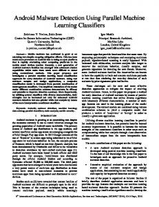


![Misleading Metrics: On Evaluating Machine Learning for Malware with ... [PDF]](https://m.moam.info/img/260x300/misleading-metrics-on-evaluating-machine-learning-_6489b596098a9e7c528b4569.jpg)