Machine learning for propensity score matching and weighting - UPF

Machine learning for propensity score matching and weighting: comparing different estimation techniques and assessing different balance diagnostics

Massimo Cannas Department of Economic and Business Sciences, University of Cagliari (Italy) Email: [email protected]

Bruno Arpino Department of Political and Social Sciences and Research and Expertise Centre for Survey Methodology, Pompeu Fabra University, Barcelona (Spain) Email: [email protected]

RECSM Working Paper Number 54 January 2018 This work is licensed under a Creative Commons Attribution 4.0 International License.

Abstract Using an extensive simulation exercise, we address two open issues in propensity score analyses: how to estimate propensity scores and how to assess covariates balance. We compare the performance of several machine learning algorithms and the standard logistic regression in terms of bias and mean squared errors of matching and weighing estimators based on the estimated propensity score. Additionally, we profit of the simulation framework to assess the ability of several measures of covariate balance in predicting the quality of the propensity score estimators in terms of bias reduction. Among the different techniques we considered, random forests performed the best when propensity scores were used for matching. In the case of weighting, both random forests and boosted tree outperformed other techniques. As for the performance of the several diagnostics of covariate balance we considered, we found that the simplest and most commonly used one, the Absolute Standardized Average Mean difference of covariates (ASAM), predicts well the bias of causal estimators. However, our findings suggest the use of a stringent rule: researchers should aim (at least) at obtaining an average ASAM lower than 10% and/or a low proportion of covariates with ASAM exceeding the 10% threshold. Balancing interactions among covariates is also desirable.

Keywords Causal inference, propensity score methods; covariate balance; machine learning algorithms; simulation study

2

1 Introduction In randomized clinical trials (RCTs) the researcher can randomize the treatment to ensure comparability of the treated and control groups by design so that unbiased estimates of the treatment can be obtained relatively easily, for example, by direct comparison of the outcome means across the two groups. Whilst RCT’s are often considered to be the gold standard for evaluation of treatment effects, in many situations it is necessary to pursue causal inference employing non experimental (or, following Cochran’s definition [1], observational) data.

Observational studies are challenging for causal inference because of the presence of imbalance in background variables affecting both the treatment and the outcome, which act as confounders. In this setting it is necessary to adjust for differences in the distributions of the observed characteristics between the treated and the control groups via matching, weighting or similar strategies. However, these approaches may be ineffective when there are many confounders. The propensity score introduced by Rosenbaum and Rubin [2] is a one-dimensional summary of the multidimensional set of covariates, with the property that, when its distribution is balanced across the treatment and control groups, the distribution of (observed) covariates is balanced in expectation across the two groups. In this way the problem of adjusting for a multivariate set of observed characteristics reduces to adjusting for the one-dimensional propensity score.

Propensity scores can be employed in several ways. Two popular methods are propensity score matching (PSM) and propensity score weighting (PSW). The reader is referred to Austin [3] and Austin and Stuart [4] for a critical review of the use of PSM and PSW in the

3

applied literature. Despite propensity score methods being widely used and extensively studied, several non-trivial issues remain open. In this paper we try to address two notable specific and interconnected problems: how to estimate propensity scores and how to assess covariates balance.

The true probability of receiving the treatment is unknown in virtually all observational studies and need to be estimated on the data. Thus, the estimated propensity score is a balancing score when we have a consistent estimate of the true propensity score, leading to what has been defined as the propensity score tautology: ―We know we have a consistent estimate of the propensity score when matching on the propensity score balances the raw covariates. Of course, once we have balance on the covariates, we are done and do not need to look back. That is, it works when it works‖ [5]. Typically a logistic regression is used to estimate propensity scores. In order to improve covariate balance, interactions terms among independent variables and nonlinear transformation of them are added [6]. Whatever the balance statistic used, this iterative process is not only laborious, but there is also no guarantee that balance improves after refinement of the propensity score [7]. Moreover applied researchers often do not follow this iterative approach [3]. Recently, the increased availability of large datasets and the parallel increase in computer capabilities opened new possibilities of analysis. Computer intensive algorithms (belonging to the broad category of machine learning methods) were first proposed for propensity score specification by D’Agostino [8] and Mc Caffrey [9]. In the context of propensity score methods, computer intensive algorithms may be useful as an automatic, data driven, way of capturing nonaddivities and nonlinearities in the estimation of the propensity score model which, on the one hand, can avoid the laborious process of specifying the logistic regression to satisfy

4

the balance property and, on the other hand, may guarantee better covariate balance. Since the formal properties of ML algorithms are usually unknown computer simulation is required to analyze their performance. Simulation is also useful to assess the relative performance of covariate balance measures. As for balance diagnostics a general suggestion is to calculate them in a way similar to the outcome analysis, for example using weights when using PSW [10]. However, several diagnostics can be considered in addition the absolute standardized average mean difference of covariates, which is the simplest and most commonly used measure of balance [4,11] but little is known about their relative performance and association with bias of causal estimate and on how to choose among them.

The aim of this paper is twofold. First, we investigate the performance in terms of bias and standard error of PSM and PSW when different types of machine learning algorithms (ML) are used to estimate the propensity score. The comparison of PSM and PSW is interesting per se because it is still debated which of the two has to be preferred [12,13]. Second, we assess the predictive power in terms of bias reduction of several measures of balance. This enables us to provide guidelines to practitioners on what covariates balance measure should be preferred for PSM and PSW and when to consider acceptable the achieved balance. We also contribute to the literature on the use of machine learning techniques in propensity score methods by comparing several algorithms in the same simulation setting, for both PSM and PSW. In the next section, after a brief review of propensity score methods, we offer a selected review of the literature focusing on the topics of covariate balance and model building strategies for propensity score estimation.

5

2 Propensity score methods 2.1 Propensity score matching and weighting The potential outcome framework, or Rubin-Holland causal model, is a recognized framework for causal inference [14]. Within this framework, several competing methods have been established and extensively studied but there also continuing developments [12]. Let T indicate a binary treatment, with T = 1 for treated units, and T = 0 for units in the control group. The potential outcome Y(T) is defined for each unit as the value of the outcome under a specific treatment condition. We assume that the potential outcomes for a unit are not affected by the treatment received by other units, and that there are no hidden versions of the treatment, which is referred to as Stable Unit Treatment Value Assumption (SUTVA)[15]. A causal estimand that is commonly of interest to estimate, and on which we focus in this paper, is the average treatment effect on the treated (ATT). Formally, ATT = EéëY (1) -Y ( 0) T =1ùû.

In observational studies, ATT is often identified invoking [16]: 1) the unconfoundedness assumption, Y (0)  T X , amounting to assume that all confounders X are observed, so that adjusting for them, Y(0) for treated units can be estimated on the sample of control units; 2) the overlap assumption, P(T  1 X )  0 , that implies that, for all possible values of the covariates, there is a positive probability of receiving the treatment. Usually, analyses are restricted to the common support of covariates across treatment groups, where this assumption is met.

6

Under these assumptions, propensity score methods can be used to estimate the ATT. The propensity score, e, is defined as the probability to receive the treatment conditional on the set of observed variables, X. Formally, e ≡ e( X ) = Pr(T = 1 | X). Rosenbaum and Rubin [2] demonstrated that if unconfoundedness holds conditional on X, it also holds conditional on e and when the propensity score distribution is balanced across the treatment and control groups, the distribution of observed covariates is balanced in expectation across the two groups (balancing property of the propensity score). This means that instead of adjusting for the multivariate set of observed variables, X, we can adjust for the one-dimensional propensity score. We consider two methods for implementing this adjustment.

Propensity score matching (PSM) consists in finding units with similar values of the propensity score across the control and treated groups. These units will form a subset of the original data, usually called matched dataset (or matched sample), where the distribution of covariates across the treatment groups will be more balanced than in the raw dataset and on which (under unconfoundedness) the ATT can be estimated as if the treatment was randomized [3,17, 18] ; see [19] for PSM with clustered data.

Propensity score weighting (PSW) aims at balancing the distribution of covariates by weighting observations using the propensity score. When the estimand of interest is the ATT it is customary to assign a weight of one to all treated units and a weight of e/(1-e) to control units. In this way the weighted set of controls will have a covariates distribution more similar to the covariates distribution of the treated units and weighted differences in

7

means of treated and control observations provide unbiased causal estimates under unconfoundedness [20,21]; see Kim et al. for PSW with clustered data [22]. In observational studies, the propensity score is typically unknown and need to be estimated. The success of both PSM and PSW depends on a good specification of the propensity score model, such that the balancing property is respected. Therefore, it is crucial to know how to improve the estimation of the propensity score and how to assess covariates balance.

2.2 The estimation of the propensity score Usually in empirical studies, a logit model is used to estimate the propensity score so that

e(X) = F ( h(X)) , where F (×) is the logistic cumulative distribution function and h(X) is a function of the covariates [2, 23]. Typically, researchers start estimating a logit model with a simple specification of h(X) and then re-estimate the model adding linear and higher order terms of covariates in an iterative process aimed at improving covariates balance. This process can be quite tedious, especially in the presence of many covariates. Frolich and Huber [24] analyzed the behavior of causal estimates under several semiparametric or non parametric specifications of h(X). In this paper we consider a class of non parametric methods for propensity score estimation, i.e. machine learning algorithms, characterized by an iterative fitting process.

8

2.2.1 Machine learning techniques for the estimation of the propensity score Machine learning (ML) algorithms were suggested as an alternative to parametric models for propensity score estimation [8, 9].

A distinctive feature of these ML algorithms is that model building is data-driven so that they can fit complex relations in an automatic way mostly overcoming variable selection and model building efforts [25]. More specifically, ML algorithms can detect automatically nonlinearities and nonadditivities. A drawback of ML model building strategy is that the fitted relation is not available in closed form and thus it is not easily interpretable. However, this loss of interpretability is not a big issue in the context of propensity score methods because the propensity score is essentially used for balancing purposes and is not of interest per se.

In short, ML algorithms can be useful to improve the performance of propensity score methods due to their flexibility, in particular when dealing with large (in terms of sample size and number of covariates) datasets. There is not a great amount of work examining ML performance for propensity score methods. Two notable contributions came from simulation studies. Setoguchi et al. [26] found that in the context of PSM, propensity score estimation via neural networks outperformed other ML algorithms (CART, Pruned CART, etc.) and logistic regression in terms of reduction of bias of ATT. Lee et al. [27] found that Boosted Regression outperformed other ML techniques (CART, Pruned CART, Random Forest) and logistic regression in the estimation of the propensity score used for PSW. The results in these two papers are only partially comparable because of the different method

9

used (PSM versus PSW) and because outcomes were of different types, binary in Lee et al. and continuous in Setoguchi et al. Moreover, the best performing techniques were not used in both papers. One of the aims of our study is to compare the ML algorithms considered in these two studies in the context of both PSM and PSW within the same simulation setting.

In the following, we give a brief description of the ML algorithms compared in our simulation studies. With the exception of neural networks and naive Bayes, we used algorithms built on Classification And Regression Trees (CART) [28]. CART algorithms that subsequently splits the data into subsets. At each step the split is defined by jointly choosing the variable and the value that minimize the variability of the outcome in the splitted data. In the simplest case the splitting procedure stops when the outcome variability in the final subsets (the so-called leaves of the tree) is sufficiently low. A more refined approach grows the tree until the maximum number of leaves is reached and then it ―prunes‖ the tree back by deleting subtrees that do not decrease much the total variability. This pruning procedure has the goal of avoiding overfitting. Since in preliminary analysis pruned trees did not perform well, to reduce the complexity of our simulation study we did not consider this method further. In addition to classification trees we also considered ensemble algorithms based on multiple trees. These algorithms use random selection features to differentiate the trees and then aggregate the results, the rationale being that averaging over several trees can improve outof-sample predictions by reducing overfitting. Bagged trees [29] are based on a large number of trees, each tree fitting a bootstrapped sample of the data of the same size of the original dataset. The prediction from the bagged tree is obtained by aggregating trees

10

estimates via majority voting. A random forest [30] is a multitude of correlated trees working in parallel but in this case the trees are correlated via random selection of both the data and the variables. More specifically, in the R implementation of the random forest that we use [31], two thirds of the data are randomly re-sampled to grow each tree and at each node the candidate splitting variables are selected among a randomly chosen subset of all predictors. The predictions are obtained by majority voting. A different modification of the CART procedure is based on the idea of ―boosting‖. Boosted trees [32] are based on the idea of incremental fitting: the algorithm is a linear combination of trees where each tree fits the residuals of the previous one using a different subsample of the data. Specific recommendations for implementing boosted trees in the context of propensity score estimation can be found in McCaffrey et al. [9] and our implementation closely follows these recommendations. Finally, we considered two non-tree based ML algorithms, i.e. neural networks and the Naïve Bayes algorithm. The latter is a very simple classifier based on Bayes theorem and an independence assumption on the covariate set. The probability of being treated conditional on covariate values is first calculated using Bayes theorem and then decomposed via independence into a product of simple conditional probabilities, each relative to a single covariate. Whilst being unrealistic in many setting, the independence assumption has been found not to be detrimental in many complex classification tasks and it guarantees a linear algorithmic complexity, making NB a remarkably fast algorithm [33]. Neural Networks are based on weighted averages of simple computing functions (units) organized in a network pattern [25]. The improvement of performance (the ―learning‖ process) is ensured by correcting weights after each instance so that the prediction error of

11

the network is minimized (backpropagation). We implemented neural networks using two layers of units as in [26].

2.3 Balance diagnostics Covariate balance can be assessed in several ways. The most commonly used measure of balance is the Absolute Standardized Average Mean difference of covariates (ASAM; [13, 34]). Some interesting properties of ASAM were highlighted by Austin [35]: i) ASAM can be bounded under the null hypothesis of perfect balance while other measures cannot, however ii) ASAM is not always sensitive to imbalance in higher moments and interactions and iii) thresholds are difficult to set as they should be sample size dependent. These findings concerned PSM but substantially similar results were recently found for PSW [4]. In general, it is difficult to fix thresholds not only on ASAM but also on other common balance measures as their distribution is generally unknown.

Some researchers suggested that ASAM should be improved without limits and warned against the risk of using tests of hypothesis of equality of means [5,35]. However, in a given sample it may be impossible to achieve a perfect balance and several rules of thumb are commonly used to assess if the final balance is acceptable. For example, an ASAM lower than 20% for each covariate is sometimes considered satisfactory [16, 36]. Others suggest a more stringent threshold of 10% [37, 38]. However, while some of these suggestions are mostly based on theoretical results based on restrictive assumptions, their appropriateness has not been extensively tested with specific simulation studies.

12

ASAM has been criticized because it only compares the means of the distributions of covariates between treated and control units. Some researchers suggested to assess ASAM also on interactions among covariates when assessing covariate balance [5, 35, 39]. Others have suggested to compare the whole distribution of covariates in the matched dataset using quantile-quantile plots (however they are not appropriate for binary variables and cannot be easily be averaged across covariates) or computing the mean and maximum difference of the empirical distribution function [5, 37]. It has to be noted that most of the previous works assessing the performance of propensity methods via simulation studies have focused on the ability of different techniques to attain a better covariate balance, as measured by one or more of the balance diagnostics available. The idea is that the better the covariate balance, the lower the bias of ATT should be. However, this is not necessarily the case as pointed out, for example, by Lee et al. [27]: “One interesting observation is that logistic regression often not only yielded the lowest ASAM but also produced large biases in the estimated treatment effect; conversely, boosted CART often did not have the lowest ASAM but frequently produced better bias reduction. This may have important implications for diagnostic methods to assess propensity score methods: is good covariate balance not enough for ensuring low bias, or is it perhaps that the ASAM is not an adequate measure of balance?” One of the key objectives of our study is to assess the strength of the association between different covariate balance diagnostics and bias of ATT. In other words, we are interested in assessing to what extent having achieved a ―good‖ level of covariate balance is predictive of achieving also a low bias of ATT. Importantly, this link must be evaluated

13

conditional on PSM or PSW. In fact, it is not obvious that similar levels of covariate balance lead to similar biases for both PSM and PSW.

3 Simulation studies 3.1 Simulation design We followed the simulation structure of Setoguchi et al. [26] as slightly modified by Lee et al. [27]. Ten basic covariates were generated from a normal distribution and transformed into four normal variables and six dummy variables with different degrees of association between them. Three covariates affected only the treatment, three only affected the outcome and four covariates affected both (so there were four confounders). A binary treatment was generated using a logistic model:

{

}

æ Pr(T =1) = ç1+ exp - f S(X ,...X ) 1 7 è

ö-1 ÷ ø

(1)

where f S models the relation between the treatment and the covariates according to treatment scenario S, using formulas provided by Setoguchi et al. [26]. The average probability of being treated is 0.5 in all scenarios. Our major addition with respect to the original simulation design was to allow for scenarios also in the outcome equation. This was done to analyse how treatment effects heterogeneity (due to increasing complexity in the link between the outcome and the covariates) affects covariates balance and bias of

14

causal estimates . Two continuous potential outcomes were generated as functions of the treatment and the covariates:

(

)

Y(T) = aTS + gS T, X ,...X , X , X , X ; 1 4 8 9 10

T = 0,1

(2)

where gS(T, X) again varies according to scenario s and the intercepts a 0Sand a1S are set to give ATT = E[Y(1)-Y(0)] = -0.4 in each scenario. Scenarios are indexed with capital letters. For example, letter A denotes the simplest scenario, i.e. when f and g are both linear in the covariates. Moving away from A the relation becomes more complex with one or more (two-way) interaction and/or quadratic terms. Table 1 gives a qualitative summary of scenarios characteristics. Detailed formulas for all scenarios are provided in the Appendix. The combination of a specific scenario for the treatment and outcome is indicated combining the two letters. For example, ―CA‖ indicates that the treatment has been generated according to a moderately nonlinear scenario (C) while the outcome has been generated using the linear scenario (A).

15

Table 1. Non additivity and non linearity in simulated treatment and outcome scenarios. A: additivity and linearity. Other scenarios have up to two (mild) or more (moderate) interactions and/or quadratic terms Scenario

A

B

C

D

E

F

G

Non additivity

none

none

none

mild

mild

moderate

moderate

Non linearity

none

mild

moderate

none

mild

none

moderate

R software (v3.21) utilities were used to generate 1000 dataset replications for each combination of scenario and size (code is available in the supplementary material). Note that treatment and outcome scenarios can combine together generating a total of 7 X 7 = 49 simulation conditions but, after preliminary results, we decided to present results for a representative sub-set of 4 X 4=16 simulation scenarios and three different dataset sizes (500, 1000 and 2000). Thus we have a total of 4 x 4 x 3 = 48 simulation conditions. In each simulated dataset, the propensity score was estimated using all covariates. The estimated propensity score was used to obtain the matched and the weighted sample, via the Matching package [40]. Since the ATT was the estimand of interest, the PSM strategy was implemented by matching (with replacement) each treated unit with the control with the most similar propensity score value. A caliper of 0.25 times the standard deviation of the estimated propensity score was used to avoid bad matches [41]. The PSW approach was

16

implemented by assigning to all treated units a weight of one and to all control units a weight of e/(1-e), a standard weighting scheme to downweight controls differing from treated and viceversa [3,4,11].

3.2 Methods to estimate the propensity score In each simulated dataset the propensity score was estimated with the following methods (in parenthesis we indicate the labels used in the graphs): o Logistic regression (only main effects; logit); o Tree (tree): classification tree obtained by recursive partitioning; rpart package o Bagged trees (bag): bootstrap aggregated tree; ipred package; o Random Forest (rf): parallel trees using repeated subsamples and randomly selected predictors; randomForest package; o Boosted trees (boost): similar to bagged tree but each tree increases weights of incorrectly classified observations in the previous tree; twang package; o Neural Network (nn): two layer; neuralnet package; o Naive Bayes (nb): package e107.

All ML algorithms were fitted in R with default parameters, even if it is possible that a fine tuning would give better results. However, since one of the principal attractiveness of ML methods is their automatic model selection we preferred to avoid fine tuning to better represent the output of these methods when used by applied researchers. The only exception was boosted trees for which we followed the recommendations of McCaffrey et

17

al. [9] in setting the tuning parameters since they were specifically targeted to causal inference applications.

3.3 Performance measures for assessing covariate balance The following statistics were used to assess balance in the matched and weighted samples obtained from each simulated dataset. In case of a weighted sample the weights were used when estimating the balance diagnostics [4]. o ASAM: The absolute average percent standardized mean difference of covariates between treated and control groups; o ASAMINT: The same as ASAM but calculated including also all possible two-way interactions.

As noticed above, ASAM should not exceed 20% for each covariate, or 10% according to a more stringent rule of thumb. Therefore, we also considered as balance measures the proportion of covariates with ASAM exceeding these two commonly used thresholds: o ASAM20: The proportion of covariates with ASAM exceeding 20%; o ASAM10: The proportion of covariates with ASAM exceeding 10%.

We then considered two measures based on the empirical distribution function:

18

o ECDFMEAN: The standardized mean difference between the quantile-quantile (QQ) plots of the covariates between treated and control groups; o ECDFMAX: The average maximum difference between the QQ plots between the treated and control groups.

The potential advantage of ECDFMEAN and ECDFMAX over the ASAM is that being these measures based on the empirical distribution function, they should capture (dis)similarities in the distribution of covariates among treated and control units not limited at their mean.

Finally, we also considered: o VARRATIO: The average (log) variance ratio of the estimated propensity score for treated and control units that should be near to one; o AUC: The area under the ROC curve of the estimated propensity score model.

3.4 Performance measures for ATT estimators To assess the performance of the different PSM and PSW estimators we considered the following average measures taken over the 500 replicates: o Relative bias (BIAS) is the absolute difference between the estimated ATT and the true ATT divided by the true ATT;

19

o Mean squared error (MSE) is the root of the average of the squared differences between ATT estimates and the true ATT. o

3.5 Measures to assess the association between balance and bias of ATT To assess the usefulness of the balance diagnostics, we considered three measures of association between the bias of ATT and each of the balance measure (in parenthesis the labels used in the graphs): o Pearson correlation coefficient (cor); o Spearman rank correlation coefficient (spe); o Kendall’s Tau (tau).

4 Results 4.1 Bias and mean squared error of ATT estimators We start by summarizing the results of our simulation experiments on the bias and MSE of ATT estimators. We focus on comparing the performance of PSW and PSM according to the techniques used for the estimation of the propensity scores.

20

In figure 1, we report the BIAS of PSW and PSM by the technique used for propensity score estimation. To keep the number of graphs shown in figure 1 manageable we averaged the results obtained for different sample sizes N for each of the 16 scenarios. First, we can notice that in each scenario and for each technique weighting always (with very few and minor exceptions) gives a smaller BIAS than matching. For the boosted (―tw‖) and bagged CART (―bag‖) the differences between the bias obtained with PSW and PSM are rather sizable in favor of PSW. Within each scenario, the techniques are in decreasing order by the overall performance in terms of BIAS, i.e., we calculated the average BIAS across all the experimental conditions and ordered the techniques. We maintain the same order throughout the paper because it is quite stable across the different experimental conditions. This is particularly true for random forest, boosted trees and logistic regression (―rf‖, ―tw‖ and ―logit‖) which generally have the best performance. We will highlight when the performance ranking deviate substantially from the general trend. In each scenario, the best performing technique is usually the random forest, both for weighting and matching. This technique also shows a remarkably stable performance across scenarios. Only in the simplest scenarios (represented in the upper-left part of Figure 1) and in case of matching, a slightly lower average BIAS is obtained with logistic regression than with random forest. However, in these cases the differences between logistic regression and random forest are rather small. The performance of the boosted trees in the case of weighting is very good and in few scenarios it is even marginally better than that of random forest (e.g., scenarios CE, CD and GD).

However, in the case of matching the performance of the boosted CART is worse as compared to weighting and the random forest performs considerably better.

21

< Figure 1 about here >

In order to show the effect of increasing the sample size, in figure 2 we report, separately for propensity score weighting and matching, the average BIAS by propensity score technique and sample size. As expected, usually as the sample size increases the BIAS reduces for all techniques used to estimate the propensity score, both for matching and weighting. However, the different techniques benefit differently from larger sample sizes. The reduction in the BIAS as the sample size increases is particularly strong for the neural network. However, also when we set the sample size to 2,000 the performance of the neural network is largely worse than that of almost all other techniques. For boosted and bagged CART the reduction of BIAS as consequence of a bigger sample size is particularly strong in the case of matching but their performance do not vary much with the sample size if used for weighting. Finally, we note that the performance of the other techniques does not seem to be particularly affected by the sample size. For each sample size, the average BIAS is lowest for random forest and boosted CART when weighting is considered. In the case of matching the performance of the boosted CART is quite poor especially for small sample sizes.

< Figure 2 about here >

Figures 3 and 4 report the performance of the different PSM and PSW estimators in terms of MSE. Overall, these figures confirm the results in the corresponding graphs we commented above for the BIAS (figures 1 and 2, respectively). Overall, PSW estimators

22

show a lower MSE than PSM estimators. The lowest MSE is usually obtained when random forest is used to estimate the propensity score. As the sample size increases, obviously the MSE decreases, especially in the case of neural network and bagged CART, which, however, perform considerably poorer than the other techniques.

< Figure 3 about here >

< Figure 4 about here >

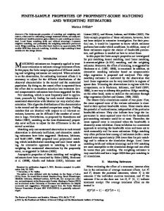
4.2 Association between balance measures and bias Because one of the goals of this study is to assess to what extent the measures of balance considered are predictive of the bias of propensity score estimators, we analyzed, both graphically and using common indexes, the association between the BIAS and several balance statistics. Each box in Figure 5 plots the BIAS and balance measure obtained after applying PSM and PSW and averaging over 500 simulated datasets. A total of 16 X 3 X 7=336 points are plotted in each graph, one for each combination of scenario, sample size and technique to estimate the propensity score. The values of the association indexes are shown on the top of each graph.

Overall, the associations between bias of ATT and balance statistics are stronger when using PSM than PSW. It is evident that AUC and VARRATIO are weakly associated with the bias, especially in the case of PSW. The remaining balance measures have similar

23

performances, even if balance measures based on ASAM show slightly stronger associations with BIAS than measures based on the empirical distribution function (ECDF). Considering that measures derived from the ECDF are not available in current statistical packages (for example in the R package Matching they are available only for PSM) the widespread use of ASAM seems justified. We also notice that ASAM INTER has a slightly better performance than ASAM. A closer look at the second graph in figure 5 that refers to the ASAM indicates that the more stringent threshold of 10% should be preferred. In fact, across all simulation conditions, on average, a mean ASAM of 10% gives a BIAS slightly lower than 20%, while a mean ASAM of 20% gives a BIAS around 35%. This graph also shows that to keep the bias very low even more stringent thresholds should be imposed.

The findings on the ASAM are complemented by those in the fourth and fifth graphs in figure 5 corresponding to the average proportion of covariates with ASAM bigger than 20% (ASAM20) or 10% (ASAM10), respectively. Results for ASAM20 indicate that even in the cases where none or a very little proportion of covariates reports an ASAM over the 20% threshold it cannot be expected, in general, to attain a low BIAS. In fact, the BIAS corresponding to values of ASAM20 near 0 show a high degree of variability including values as high as 40%. A different picture is shown in the fifth graph of figure 5 corresponding to ASAM10. In this case, all simulation conditions where ASAM10 is, on average, equal or very close to 0, the BIAS is considerably low.

< Figure 5 about here >

24

5 Discussion Methods based on the propensity score are widely adopted by researchers in several applied fields [11,16]. However, the implementation of these methods poses some important questions that are still debated in the literature. In this paper, using a series of Monte Carlo simulations, we addressed two essential specific and interconnected problems: how to estimate the propensity score and how to assess covariates balance both in the context of matching and weighting using the estimated propensity scores. The first goal of this paper was to examine the bias of propensity score matching and weighting depending on the technique used for the estimation of the propensity score. Building on previous studies [26, 27] we compared the standard logistic regression model with several machine learning techniques. We confirmed that machine learning techniques are useful to improve propensity score estimation. By comparing the performance of several machine learning techniques in the same simulation setting and both for propensity score matching and weighting we significantly add to previous studies. In fact, our simulation results point to the fact that boosted CART, that was the preferred ML techniques in the simulation study by Lee et al. [27] is confirmed to perform very well when propensity scores are using for weighting. However, under several simulation conditions, we found that random forest performed similarly well or even better than boosted CART in the context of propensity score weighting. When propensity score matching is considered, random forest always performed considerably better than boosted CART and the other techniques. Overall, our simulations suggest that the random forest should be preferred as it often guarantees the lowest bias and in the other cases its performance is not substantially different than those of the other best performing

25

techniques. Moreover, the random forest has the advantage that its implementation is much quicker than that of the boosted CART.

The second aim of our study was to assess the association between the values of several balance diagnostic and the bias of ATT in order to appreciate the ability of the different measures in predicting the bias of propensity score based estimators of ATT. We compared the simple absolute average percent standardized mean difference of covariates between treated and control groups (ASAM) with other measures. Some of these alternative diagnostics are refinements of the basic ASAM because of the inclusion of all interactions terms among covariates in its calculation or because of considering the proportion of covariates with ASAM exceeding a given threshold (20% or 10%). We also considered alternative covariate balance diagnostics: two measures based on comparing the whole distribution of covariates using the empirical cumulative distribution function; the average (log) variance ratio of the estimated propensity score for treated and control units (VARRATIO); the area under the ROC curve of the estimated propensity score (AUC). We found that the simple ASAM is a good measure of covariate balance because it predicts well the bias of ATT. The values of the ASAM obtained varying the different simulation conditions and with different techniques were, in fact, strongly associated with the values of the bias of ATT. Including interactions among covariates in the calculation of the average ASAM (ASAM INTER) slightly improved the assessment of covariate balance. Given that including interactions in the calculation of ASAM can be implemented very easily and that it can improve the assessment of covariate balance, especially in the presence of nonlinearities in the effect of covariates, we recommend the use of ASAM INTER.

26

While the average ASAM calculated on all covariates seems to be a good diagnostic, our results point to the importance of considering (additionally to the average ASAM) the balance of each covariate separately. In fact, important insights are gained when considering the proportion of covariates exceeding 20% or 10% of ASAM (ASAM20 and ASAM10, respectively). We found that in many cases where the proportion of covariates with ASAM exceeding 20%, the bias of ATT was high suggesting that the 20% threshold may be too lax. Our results indicate that the stricter 10% threshold is more appropriate. Indeed, when ASAM10 was 0 or very close to 0, the bias of ATT was always very low.

Diagnostics based on comparing quantile-quantile plots showed similar associations with the bias of ATT as those of the ASAM-based measures. Given that these measures are not implemented in standard software, the use of the simplest measures based on the ASAM seems justified based on our findings. The other two measures we considered, VARRATIO and AUC performed quite poorly in predicting the bias of ATT estimators. The VARRATIO is essentially a measure of overlap [42, 16] so its low correlation with the bias of ATT is not surprising given that in our simulation we have overlap by construction. AUC measures the goodness of fit of the PS model and its poor performance as a diagnostic of covariate balance confirms that when using propensity scores methods we should not care about model fit but only about covariate balance [23].

Based on our simulation results, we also noticed that the associations between bias of ATT and the values of covariate balance diagnostics were stronger when using PSM than PSW. This may suggest that practitioners should use more severe rules for the assessment of covariate balance when using PSW.

27

As all simulation studies, we were limited in the number of simulation conditions we have generated. However, in our simulations we varied the sample size, the degree of nonlinearity and nonadditivity of the effects of covariates in the treatment equations and, differently from previous studies, we also allowed for nonlinearity and nonadditivity in the potential outcome equations, permitting treatment effects heterogeneities.

Summarizing, from our simulation study we can derive two key messages for applied researches interested in applying PSM and PSW in observational studies. First, we confirm the utility of machine learning techniques for the estimation of propensity score. More specifically, we found that PSM and PSW based on random forests for the estimation of the propensity score performed considerably well in terms of bias and MSE of ATT. Second, we found that the simplest and most commonly used covariate balance diagnostic, the ASAM, is a good measure of covariate balance because it predicts well the bias of ATT. However, our findings suggest the use of a stringent rule: we should aim (at least) at obtaining an average ASAM lower than 10% and/or a low proportion of covariates with ASAM exceeding the 10% threshold. This rule can, of course, be combined with substantive knowledge, that could suggest being more rigorous with some particular covariates that may be expected to be prognostically more important than others [4].

28

References 1. Cochran WG The planning of observational studies of human populations (with discussion), Journal of the Royal Statistical Society (Series A) 1965; 128: 134—155.

2. Rosenbaum PR, Rubin DB. The central role of the propensity score in observational studies for causal effects. Biometrika 1983; 70: 41–55.

3. Austin PC. A critical review of propensity score matching in the medical literature between 1996 and 2003. Statistics in Medicine 2008; 27: 2037-2049.

4. Austin PC, Stuart E. Moving towards best practice when using inverse probability of treatment weighting (IPTW) using the propensity score to estimate causal treatment effects in observational studies. Statistics in medicine 2015; 34: 3661-3679.

5. Ho DE, Imai K, King G, Stuart EA. Matching as nonparametric preprocessing for reducing model dependence in parametric causal inference. Political Analysis 2007; 15:199–236. 6. Rosenbaum PR, Rubin DB Reducing bias in observational studies using subclassification on the propensity score. Journal of the American Statistical Association 1984; 79:516–524.

7. Diamond A, Sekhon JS. Genetic matching for estimating causal effects: A general multivariate matching method for achieving balance in observational studies. Review of Economics and Statistics, 2013; 95(3): 932-945.

29

8. D’Agostino Jr RB. Propensity score methods for bias reduction in the comparison of a treatment to a non-randomized control group. Statistics in Medicine 1998; 17(19): 22652281.

9. McCaffrey DF, Ridgeway G, Morral AR. Propensity score estimation with boosted regression for evaluating causal effects in observational studies. Psychological Methods 2004; 9(4): 403–425.

10. Joffe MM, Ten Have TR, Feldman HI, Kimmel SE. Model selection, confounder control, and marginal structural models. The American Statistician 2004; 58(4): 272–279.

11. Austin, PC. The relative ability of different propensity-score methods to balance measured covariates between treated and untreated subjects in observational studies. Medical Decision Making 2009, 29, 661–677. 12. Athey S, Imbens GW. The state of applied Econometrics – Causality and Policy Evaluation. ArXiv 2016; 1607.00699v1.

13. Busso M, DiNardo J, McCrary J. New Evidence on the Finite Sample Properties of Propensity Score Reweighting and Matching Estimators. unpublished manuscript 2013.

14. Holland PW. Statistics and Causal Inference. Journal of the American Statistical Association 1986; 81(396): 945-960.

30

15. Rubin DB. Randomization Analysis of Experimental Data: The Fisher Randomization Test Comment. Journal of the American Statistical Association 1980; 75: 591–593.

16. Imbens GW, Rubin DB. Causal inference in statistics, social, and biomedical sciences. Cambridge University Press, 2015.

17. Stuart EA. Matching methods for causal inference: A review and a look forward. Statistical science: a review journal of the Institute of Mathematical Statistics 2010; 25(1): 1-34.

18. Dettmann E, Becker C, Schmeißer C. Distance functions for matching in small samples. Computational Statistics & Data Analysis 2011, 55(5) 2011, 1942-1960

19. Arpino B, Cannas M. Propensity score matching with clustered data. An application to the estimation of the impact of caesarean section on the Apgar score. Statistics in Medicine 2016, 35(12), 2074–2091

20. Curtis LH, Hammill BG, Eisenstein EL et al. Using inverse probability-weighted estimators in comparative effectiveness analyses with observational databases. Medical Care 2007; 45(10):103-107.

21. Lunceford JK, Davidian M. Stratification and weighting via the propensity score in estimation of causal treatment effects: a comparative study. Statistics in Medicine 2004; 23(19): 2937-2960.

31

22. Kim GS, Paik CM, Kim H. Causal inference with observational data under clusterspecific non-ignorable assignment mechanism. Computational Statistics & Data Analysis 2017; 113: 88-99.

23. Rubin DB. On principles for modeling propensity scores in medical research. Pharamacoepidemiology and drug safety 2004; 13(12): 855-857.

24. Frölich M, Huber M, Wiesenfarth M. The finite sample performance of semi- and nonparametric estimators for treatment effects and policy evaluation. Computational Statistics & Data Analysis 2017; 115: 91-102.

25. Ripley BD. Pattern Recognition and Neural Networks. Cambridge University Press, 2008

26. Setoguchi S, Schneeweiss S, Brookhart MA et al. Evaluating uses of data mining techniques in propensity score estimation: a simulation study. Pharmacoepidemiology and Drug Safety 2008; 17(6): 546–555.

27. Lee BK, Lessler J, Stuart EA. Improving propensity score weighting using machine learning. Statistics in medicine 2010; 29(3): 337-346.

28. Breiman L, Friedman J, Olshen R and Stone C. Classification and Regression Trees. Wadsworth Belmont 1984, California.

32

29. Breiman L. Bagging predictors, Machine Learning 1996; 24(2): 123-140.

30. Breiman L. Random forests, Machine Learning 2001; 45: 5-32.

31. Liaw A and Wiener M. Classification and Regression by RandomForest. R News 2001; 2, 18-22.

32. Friedman J, Jerome H. Greedy function approximation: A gradient boosting machine. Annals of Statistics, 2001; 5: 1189—1232.

33. Ng AY, Jordan MI. On discriminative vs. generative classifiers: A comparison of logistic regression and naive Bayes. Advances in Neural Information Processing Systems (NIPS) 2002 (14).

34. Rosenbaum PR, Rubin DB. Constructing a control group using multivariate matched sampling methods that incorporate the propensity score. The American Statistician 1986; 40:249–251.

35. Imai K, King G, Stuart EA. Misunderstandings among experimentalists and observationalists: balance test fallacies in causal inference. Journal of The Royal Statistical Society – Series A 2006; 171(2): 481:502.

36. Cochran WG. The effectiveness of adjustment by subclassification in removing bias in observational studies. Biometrics 1968; 24: 295-313.

33

37. Austin PC. Balance diagnostics for comparing the distribution of baseline covariates between treatment groups in propensity-score matched samples Statistics in medicine 2009; 28: 3083-3107.

38. Normand SL, Landrum MB, Guadagnoli E et al. Validating recommendations for coronary angiography following acute myocardial infarction in the elderly: a matched analysis using propensity scores. Journal of Clinical Epidemiology 2001; 54: 387–398.

39. Rubin DB. Using propensity scores to help design observational studies: application to the tobacco litigation. Health Services and Outcomes Research Methodology 2001; 2(3–4): 169–188.

40. Sekhon JS. Multivariate and propensity score matching software with automated balance optimization: the Matching package for R. Journal of Statistical Software 2011; 42(7): 1—52.

41. Austin PC. Optimal caliper widths for propensity‐score matching when estimating differences in means and differences in proportions in observational studies. Pharmaceutical statistics 2011; 10(2): 150-161.

42. Cochran WG, Rubin DB. Controlling bias in observational studies: a review. Sankhya A 1973; 35: 417– 446.

34

Appendix: Exact formulae for the data generating models In this appendix we report specifications of the treatment and outcome equations (1) and (2).

Scenario A (baseline: additivity and linearity in both treatment and outcome equation) 7 f A (X) = å b X i i i =1

gA (T, X) = aT +

a X å T,i i i =1,...4,8,...10

T = 0,1

,

Other scenarios in the treatment equation

f B ( X )  f A ( X )   2 X 22 (mild non linearity)

f C ( X )  f A ( X )   2 X 22   4 X 42   7 X 72 (moderate non linearity)

f D ( X )  f A ( X )  0.51 X 1 X 3  0.5 2 X 2 X 4  0.7 4 X 4 X 5  0.5 5 X 5 X 6 (mild non additivity)

f E ( X )  f A ( X )   2 X 22  0.51 X 1 X 3  0.5 2 X 2 X 4  0.7 4 X 4 X 5  0.5 5 X 5 X 6 (mild non additivity and non linearity)

35

f F  f A ( X )  0.51 X 1 X 3  0.7  2 X 2 X 4  0.5 3 X 3 X 5  0.7  4 X 4 X 6  0.5 5 X 5 X 7   0.51 X 1 X 6  0.7  2 X 2 X 3  0.5 3 X 3 X 4  0.5 4 X 4 X 5  0.5 5 X 5 X 6

(moderate non additivity)

f G = f A (X) + b2 X22 + b4 X42 + b7 X72 + 0.5b1 X1 X3 + 0.7b2 X2 X4 + 0.5b3 X3 X5 + 0.7b4 X4 X6 + + 0.5b5 X5 X7 + 0.5b1 X1 X6 + 0.7b2 X2 X3 + 0.5b3 X3 X4 + 0.5b4 X4 X5 + 0.5b5 X5 X6 (moderate non additivity and non linearity)

Other scenarios in the outcome equation:

gB(T = 0, X) = gA (0, X) + 0.5a 2 X22 gB(T =1, X) = gA (1, X) + a 2 X22

gC (T = 0, X) = gA (0, X) + 0.5a 2 X22 + 0.5a 4 X42 gC (T =1, X) = gA (1, X) + a 2 X22 + a 4 X42

gD (T = 0, X) = gA (0, X) gD (T =1, X) = gA (1, X) + 0.25a 2 X2 + 0.25a 4 X4

36

gE (T = 0, X) = gA (0, X) gE (T = 1, X) = gA (1, X) + 0.25a 2 X2 + 0.25a 4 X4

gF (T = 0, X) = gA (0, X) gF (T =1, X) = gA (1, X) + 2a 2 X2 + 2a3 X3 + 2a 4 X4

gG (T = 0, X) = gA (0, X) + 0.1a1 X22 + 0.1a 4 X42 gG (T = 1, X) = gA (1, X) + 0.25a 2 X2 + 0.25a 4 X4 + 0.025a1 X22 + 0.025a 4 X42

37

Figure 1 – Bias of ATT estimators by scenario, method (PSM or PSW) and technique for the estimation of the propensity score (on the x-axis). treatment equation scenarios

logit

rf

tw

bag tree

nn

nb

logit

rf

tw

bag tree

nn

nb

bag tree

nn

nb

logit

rf

tw

bag tree

nn

nb

logit

rf

tw

bag tree

nn

nb

50 0 10

30

50 30 tw

tw

bag tree

nn

nb

logit

rf

tw

bag tree

nn

nb

logit

rf

tw

bag tree

nn

nb

logit

rf

tw

bag tree

nn

nb

30 30

50

0 10

30

50

0 10

30 30

50

0 10

30

50

0 10

30 30

50

0 10

C

rf

rf

logit

rf

tw

bag tree

nn

nb

logit

rf

tw

bag tree

nn

nb

logit

rf

tw

bag tree

nn

nb

logit

rf

tw

bag tree

nn

nb

38

0 10

0 10

0 10

F

30

50

0 10

D

logit

logit

50

nb

nb

30

nn

nn

0 10

bag tree

bag tree

50

tw

tw

30

rf

rf

0 10

logit

logit

50

nb

30

nn

50

bag tree

50

tw

D

0 10

30 0 10

30

A

0 10

rf

50

logit

0 10

outcome equation scenarios

C

50

B

50

A

Figure 2 – Bias of ATT estimators by technique for the estimation of the propensity score, method (PSM or PSW) and sample size (on the x-axis).

1000

2000

500

1000

500

1000

tree

nn

nb

10 20 30 40 50 60 70

N

1000 N

2000

10 20 30 40 50 60 70 2000

500

1000

2000

1000 N

39

1000

Weigthing

500

N

500

2000

N

0

10 20 30 40 50 60 70

N

0 500

bag

0

10 20 30 40 50 60 70 2000

N

0

10 20 30 40 50 60 70

500

tw

0

10 20 30 40 50 60 70

rf

0

0

10 20 30 40 50 60 70

logit

2000

Matching

Figure 3 – Mean Squared Error of ATT estimators by scenario, method (PSM or PSW) and technique for the estimation of the propensity score (on the x-axis).

treatment equation scenarios

0.06 0.04

0.04

0.04 nb

logit

rf

tw

bag tree

nn

nb

logit

rf

tw

bag tree

nn

nb

tw

bag tree

nn

nb

logit

rf

tw

bag tree

nn

nb

logit

rf

tw

bag tree

nn

nb

0.02 logit

rf

tw

bag tree

nn

nb

logit

rf

tw

bag tree

nn

nb

logit

rf

tw

bag tree

nn

nb

0.04

0.04

logit

rf

tw

bag tree

nn

nb

logit

rf

tw

bag tree

nn

nb

logit

rf

tw

bag tree

nn

nb

nn

nb

0.02 0.04

0.06

0.00

0.02 0.04

0.06

0.00

0.02 0.00 0.06 0.04

0.02 0.06

0.00

0.02

Weigthing

Matching

0.04

0.04

0.06

0.00

0.02 0.00 0.06 0.04

0.04

0.06

0.00

0.02

D

0.04

0.06

0.00

0.02

C

0.04

0.00

0.02 rf

logit

rf

tw

bag tree

nn

nb

logit

rf

tw

bag tree

nn

nb

0.02 0.00

0.02 0.00

0.00

0.02

F 0.02 0.00

outcome equation scenarios

logit

0.06

nn

0.04

bag tree

0.06

tw

0.06

rf

0.06

logit

0.00

0.02 0.00

0.00

0.02

A

0.04

D

0.06

C

0.06

B

0.06

A

logit

40

rf

tw

bag tree

nn

nb

logit

rf

tw

bag tree

Figure 4 – Mean Squared Error of ATT estimators by technique for the estimation of the propensity score, method (PSM or PSW) and sample size (on the x-axis).

2000

500

1000

0.06 0.04 0.00

2000

500

1000

nb

1000 N

2000

2000

1000

1000

Weigthing

0.02 500

500

2000

500

N

1000 N

41

2000

N

0.00

0.02 0.00

0.02

0.06

nn

0.04

tree 0.06

N

0.04

N

0.06

N

0.00 500

0.02

0.04 0.00

0.02

0.04 0.00

0.02

0.04 0.02 0.00

1000

0.04

500

bag

0.06

tw

0.06

rf

0.06

logit

2000

Matching

Figure 5: Association between measures of covariate balance and bias of ATT. Each scatterplot shows pairs obtained from PSM (gray) and PSW (black) for each combination of scenario, dataset size and PS method, averaged over 1000 simulated datasets.

Weighting: cor = 0.835

tau = 0.552

spe = 0.738

Weighting: cor = 0.853

tau = 0.621

spe = 0.812

spe = 0.627

Matching: cor = 0.93

tau = 0.686

spe = 0.865

Matching: cor = 0.934

tau = 0.719

spe = 0.884

0.1

0.2

0.3

0.4

0.5

0.6

0.7

60 0

20

40

60 0

20

40

60 40 0

20

BIAS

80

spe = 0.141

tau = 0.453

80

tau = 0.093

Matching: cor = 0.578

80

Weighting: cor = 0.276

0

10

20

auc

40

5

10

15

20

25

30

tau = 0.561

spe = 0.75

Weighting: cor = 0.831

tau = 0.555

spe = 0.744

Matching: cor = 0.921

tau = 0.677

spe = 0.858

Matching: cor = 0.929

tau = 0.699

spe = 0.873

10

15

20

60 0

20

40

60 40 0

0

20

40

60

80

Weighting: cor = 0.837

spe = 0.838

80

spe = 0.784

tau = 0.655

80

tau = 0.598

Matching: cor = 0.888

5

0

5

10

15

20

25

30

asam10 spe = 0.764

tau = 0.687

spe = 0.861

Weighting: cor = 0.277 Matching: cor = 0.767

tau = -0.041

spe = -0.073

tau = 0.449

spe = 0.636

60 20 0

0.10

0.15

0.20

0.25

0.02

0.04

0.06

Weigthing

40

60 40 20 0

0.05

0.00

0.0

0.1

ecdfmax

0.2

varratio

42

0.08

ecdfmean

80

tau = 0.572

Matching: cor = 0.925

80

Weighting: cor = 0.825

35

asamint

Weighting: cor = 0.798

asam20

0.00

0

asam

20

BIAS

0

BIAS

30

0.3

0.4

Matching

0.10

0.12