Machine Learning Group Computer Science Department Universite ...

Handbook Statistical foundations of machine learning Gianluca Bontempi Machine Learning Group Computer Science Department Universite Libre de Bruxelles, ULB Belgique

2

Contents Index

2

1 Introduction 1.1 Notations . . . . . . . . . . . . . . . . . . . . . . . . . . . . . . . . .

9 15

2 Foundations of probability 2.1 The random model of uncertainty . . . . . . . . . . . . . . . . . . . . 2.1.1 Axiomatic definition of probability . . . . . . . . . . . . . . . 2.1.2 Symmetrical definition of probability . . . . . . . . . . . . . . 2.1.3 Frequentist definition of probability . . . . . . . . . . . . . . 2.1.4 The Law of Large Numbers . . . . . . . . . . . . . . . . . . . 2.1.5 Independence and conditional probability . . . . . . . . . . . 2.1.6 Combined experiments . . . . . . . . . . . . . . . . . . . . . . 2.1.7 The law of total probability and the Bayes’ theorem . . . . . 2.1.8 Array of joint/marginal probabilities . . . . . . . . . . . . . . 2.2 Random variables . . . . . . . . . . . . . . . . . . . . . . . . . . . . . 2.3 Discrete random variables . . . . . . . . . . . . . . . . . . . . . . . . 2.3.1 Parametric probability function . . . . . . . . . . . . . . . . . 2.3.2 Expected value, variance and standard deviation of a discrete r.v. . . . . . . . . . . . . . . . . . . . . . . . . . . . . . . . . . 2.3.3 Moments of a discrete r.v. . . . . . . . . . . . . . . . . . . . . 2.3.4 Entropy and relative entropy . . . . . . . . . . . . . . . . . . 2.4 Continuous random variable . . . . . . . . . . . . . . . . . . . . . . . 2.4.1 Mean, variance, moments of a continuous r.v. . . . . . . . . . 2.5 Joint probability . . . . . . . . . . . . . . . . . . . . . . . . . . . . . 2.5.1 Marginal and conditional probability . . . . . . . . . . . . . . 2.5.2 Entropy in the continuous case . . . . . . . . . . . . . . . . . 2.6 Common discrete probability functions . . . . . . . . . . . . . . . . . 2.6.1 The Bernoulli trial . . . . . . . . . . . . . . . . . . . . . . . . 2.6.2 The Binomial probability function . . . . . . . . . . . . . . . 2.6.3 The Geometric probability function . . . . . . . . . . . . . . 2.6.4 The Poisson probability function . . . . . . . . . . . . . . . . 2.7 Common continuous distributions . . . . . . . . . . . . . . . . . . . . 2.7.1 Uniform distribution . . . . . . . . . . . . . . . . . . . . . . . 2.7.2 Exponential distribution . . . . . . . . . . . . . . . . . . . . . 2.7.3 The Gamma distribution . . . . . . . . . . . . . . . . . . . . 2.7.4 Normal distribution: the scalar case . . . . . . . . . . . . . . 2.7.5 The chi-squared distribution . . . . . . . . . . . . . . . . . . 2.7.6 Student’s t-distribution . . . . . . . . . . . . . . . . . . . . . 2.7.7 F-distribution . . . . . . . . . . . . . . . . . . . . . . . . . . . 2.7.8 Bivariate continuous distribution . . . . . . . . . . . . . . . . 2.7.9 Correlation . . . . . . . . . . . . . . . . . . . . . . . . . . . .

19 19 21 21 22 22 24 25 27 27 29 30 31

3

31 33 33 34 35 35 37 38 39 39 39 39 40 41 41 41 41 42 43 44 44 45 46

4

CONTENTS 2.7.10 Mutual information . . . . . . . . 2.8 Normal distribution: the multivariate case 2.8.1 Bivariate normal distribution . . . 2.9 Linear combinations of r.v. . . . . . . . . 2.9.1 The sum of i.i.d. random variables 2.10 Transformation of random variables . . . 2.11 The central limit theorem . . . . . . . . . 2.12 The Chebyshev’s inequality . . . . . . . .

. . . . . . . .

. . . . . . . .

. . . . . . . .

. . . . . . . .

. . . . . . . .

. . . . . . . .

. . . . . . . .

. . . . . . . .

. . . . . . . .

. . . . . . . .

. . . . . . . .

. . . . . . . .

. . . . . . . .

. . . . . . . .

. . . . . . . .

47 48 49 51 51 52 52 53

3 Classical parametric estimation 3.1 Classical approach . . . . . . . . . . . . . . . . 3.1.1 Point estimation . . . . . . . . . . . . . 3.2 Empirical distributions . . . . . . . . . . . . . . 3.3 Plug-in principle to define an estimator . . . . 3.3.1 Sample average . . . . . . . . . . . . . . 3.3.2 Sample variance . . . . . . . . . . . . . 3.4 Sampling distribution . . . . . . . . . . . . . . 3.5 The assessment of an estimator . . . . . . . . . 3.5.1 Bias and variance . . . . . . . . . . . . . ˆ . . . . . . . . . . 3.5.2 Bias and variance of µ ˆ2 . . . . . . . . . 3.5.3 Bias of the estimator σ 3.5.4 Bias/variance decomposition of MSE . . 3.5.5 Consistency . . . . . . . . . . . . . . . . 3.5.6 Efficiency . . . . . . . . . . . . . . . . . 3.5.7 Sufficiency . . . . . . . . . . . . . . . . . 3.6 The Hoeffding’s inequality . . . . . . . . . . . . 3.7 Sampling distributions for Gaussian r.v.s . . . . 3.8 The principle of maximum likelihood . . . . . . 3.8.1 Maximum likelihood computation . . . 3.8.2 Properties of m.l. estimators . . . . . . 3.8.3 Cramer-Rao lower bound . . . . . . . . 3.9 Interval estimation . . . . . . . . . . . . . . . . 3.9.1 Confidence interval of µ . . . . . . . . . 3.10 Combination of two estimators . . . . . . . . . 3.10.1 Combination of m estimators . . . . . . 3.11 Testing hypothesis . . . . . . . . . . . . . . . . 3.11.1 Types of hypothesis . . . . . . . . . . . 3.11.2 Types of statistical test . . . . . . . . . 3.11.3 Pure significance test . . . . . . . . . . . 3.11.4 Tests of significance . . . . . . . . . . . 3.11.5 Hypothesis testing . . . . . . . . . . . . 3.11.6 Choice of test . . . . . . . . . . . . . . . 3.11.7 UMP level-α test . . . . . . . . . . . . . 3.11.8 Likelihood ratio test . . . . . . . . . . . 3.12 Parametric tests . . . . . . . . . . . . . . . . . 3.12.1 z-test (single and one-sided) . . . . . . . 3.12.2 t-test: single sample and two-sided . . . 3.12.3 χ2 -test: single sample and two-sided . . 3.12.4 t-test: two samples, two sided . . . . . . 3.12.5 F-test: two samples, two sided . . . . . 3.13 A posteriori assessment of a test . . . . . . . . 3.13.1 Receiver Operating Characteristic curve

. . . . . . . . . . . . . . . . . . . . . . . . . . . . . . . . . . . . . . . . . .

. . . . . . . . . . . . . . . . . . . . . . . . . . . . . . . . . . . . . . . . . .

. . . . . . . . . . . . . . . . . . . . . . . . . . . . . . . . . . . . . . . . . .

. . . . . . . . . . . . . . . . . . . . . . . . . . . . . . . . . . . . . . . . . .

. . . . . . . . . . . . . . . . . . . . . . . . . . . . . . . . . . . . . . . . . .

. . . . . . . . . . . . . . . . . . . . . . . . . . . . . . . . . . . . . . . . . .

. . . . . . . . . . . . . . . . . . . . . . . . . . . . . . . . . . . . . . . . . .

. . . . . . . . . . . . . . . . . . . . . . . . . . . . . . . . . . . . . . . . . .

. . . . . . . . . . . . . . . . . . . . . . . . . . . . . . . . . . . . . . . . . .

. . . . . . . . . . . . . . . . . . . . . . . . . . . . . . . . . . . . . . . . . .

. . . . . . . . . . . . . . . . . . . . . . . . . . . . . . . . . . . . . . . . . .

. . . . . . . . . . . . . . . . . . . . . . . . . . . . . . . . . . . . . . . . . .

55 55 57 57 58 59 59 59 61 61 62 63 65 65 66 66 67 67 68 69 72 72 73 73 76 77 78 78 78 79 79 81 82 83 84 84 85 86 87 87 87 88 89

CONTENTS

5

4 Nonparametric estimation and testing 4.1 Nonparametric methods . . . . . . . . . . 4.2 Estimation of arbitrary statistics . . . . . 4.3 Jacknife . . . . . . . . . . . . . . . . . . . 4.3.1 Jacknife estimation . . . . . . . . . 4.4 Bootstrap . . . . . . . . . . . . . . . . . . 4.4.1 Bootstrap sampling . . . . . . . . 4.4.2 Bootstrap estimate of the variance 4.4.3 Bootstrap estimate of bias . . . . . 4.5 Bootstrap confidence interval . . . . . . . 4.5.1 The bootstrap principle . . . . . . 4.6 Randomization tests . . . . . . . . . . . . 4.6.1 Randomization and bootstrap . . . 4.7 Permutation test . . . . . . . . . . . . . . 4.8 Considerations on nonparametric tests . .

. . . . . . . . . . . . . .

. . . . . . . . . . . . . .

. . . . . . . . . . . . . .

. . . . . . . . . . . . . .

. . . . . . . . . . . . . .

. . . . . . . . . . . . . .

5 Statistical supervised learning 5.1 Introduction . . . . . . . . . . . . . . . . . . . . . . . 5.2 Estimating dependencies . . . . . . . . . . . . . . . . 5.3 The problem of classification . . . . . . . . . . . . . 5.3.1 Inverse conditional distribution . . . . . . . . 5.4 The problem of regression estimation . . . . . . . . . 5.4.1 An illustrative example . . . . . . . . . . . . 5.5 Generalization error . . . . . . . . . . . . . . . . . . 5.5.1 The decomposition of the generalization error 5.5.2 The decomposition of the generalization error 5.6 The supervised learning procedure . . . . . . . . . . 5.7 Validation techniques . . . . . . . . . . . . . . . . . . 5.7.1 The resampling methods . . . . . . . . . . . . 5.8 Concluding remarks . . . . . . . . . . . . . . . . . . 6 The 6.1 6.2 6.3 6.4 6.5 6.6

. . . . . . . . . . . . . .

. . . . . . . . . . . . . .

. . . . . . . . . . . . . .

. . . . . . . . . . . . . .

. . . . . . . . . . . . . .

. . . . . . . . . . . . . .

. . . . . . . . . . . . . .

91 . 91 . 92 . 93 . 93 . 95 . 95 . 95 . 96 . 97 . 98 . 99 . 101 . 101 . 102

. . . . . . . . . . . . . . . . . . . . . . . . . . . . . . . . . . . . . . . . . . . . . . . . . . . . . . . . . . . . . . . in regression . in classification . . . . . . . . . . . . . . . . . . . . . . . . . . . . . . . . . . . .

105 105 108 110 112 114 114 117 117 120 121 122 122 124

. . . . . . . . . . . . .

. . . . . . . . . . . . .

. . . . . . . . . . . . .

. . . . . . . . . . . . .

. . . . . . . . . . . . .

. . . . . . . . . . . . .

. . . . . . . . . . . . .

. . . . . . . . . . . . .

. . . . . . . . . . . . .

. . . . . . . . . . . . .

. . . . . . . . . . . . .

125 125 126 126 126 127 128 128 128 132 133 134 138 139

7 Linear approaches 7.1 Linear regression . . . . . . . . . . . . . . . . . . . 7.1.1 The univariate linear model . . . . . . . . . 7.1.2 Least-squares estimation . . . . . . . . . . . 7.1.3 Maximum likelihood estimation . . . . . . . 7.1.4 Partitioning the variability . . . . . . . . . 7.1.5 Test of hypotheses on the regression model 7.1.6 Interval of confidence . . . . . . . . . . . .

. . . . . . .

. . . . . . .

. . . . . . .

. . . . . . .

. . . . . . .

. . . . . . .

. . . . . . .

. . . . . . .

. . . . . . .

. . . . . . .

141 141 141 142 144 145 145 146

6.7

6.8

machine learning procedure Introduction . . . . . . . . . . . Problem formulation . . . . . . Experimental design . . . . . . Data pre-processing . . . . . . The dataset . . . . . . . . . . . Parametric identification . . . . 6.6.1 Error functions . . . . . 6.6.2 Parameter estimation . Structural identification . . . . 6.7.1 Model generation . . . . 6.7.2 Validation . . . . . . . . 6.7.3 Model selection criteria Concluding remarks . . . . . .

. . . . . . . . . . . . . .

. . . . . . . . . . . . .

. . . . . . . . . . . . .

. . . . . . . . . . . . .

. . . . . . . . . . . . .

. . . . . . . . . . . . .

. . . . . . . . . . . . .

. . . . . . . . . . . . .

. . . . . . . . . . . . .

. . . . . . . . . . . . .

. . . . . . . . . . . . .

6

CONTENTS . . . . . . . . . . . . . . . .

. . . . . . . . . . . . . . . .

. . . . . . . . . . . . . . . .

. . . . . . . . . . . . . . . .

. . . . . . . . . . . . . . . .

. . . . . . . . . . . . . . . .

. . . . . . . . . . . . . . . .

. . . . . . . . . . . . . . . .

. . . . . . . . . . . . . . . .

. . . . . . . . . . . . . . . .

146 150 150 150 151 153 153 153 154 156 158 160 161 164 168 170

8 Nonlinear approaches 8.1 Nonlinear regression . . . . . . . . . . . . . . . . . . 8.1.1 Artificial neural networks . . . . . . . . . . . 8.1.2 From global modeling to divide-and-conquer . 8.1.3 Classification and Regression Trees . . . . . . 8.1.4 Basis Function Networks . . . . . . . . . . . . 8.1.5 Radial Basis Functions . . . . . . . . . . . . . 8.1.6 Local Model Networks . . . . . . . . . . . . . 8.1.7 Neuro-Fuzzy Inference Systems . . . . . . . . 8.1.8 Learning in Basis Function Networks . . . . . 8.1.9 From modular techniques to local modeling . 8.1.10 Local modeling . . . . . . . . . . . . . . . . . 8.2 Nonlinear classification . . . . . . . . . . . . . . . . . 8.2.1 Naive Bayes classifier . . . . . . . . . . . . . 8.2.2 SVM for nonlinear classification . . . . . . . .

. . . . . . . . . . . . . .

. . . . . . . . . . . . . .

. . . . . . . . . . . . . .

. . . . . . . . . . . . . .

. . . . . . . . . . . . . .

. . . . . . . . . . . . . .

. . . . . . . . . . . . . .

. . . . . . . . . . . . . .

. . . . . . . . . . . . . .

177 179 180 187 188 193 193 194 196 196 201 201 212 212 214

9 Model averaging approaches 9.1 Stacked regression . . . . . . . . 9.2 Bagging . . . . . . . . . . . . . . 9.3 Boosting . . . . . . . . . . . . . . 9.3.1 The Ada Boost algorithm 9.3.2 The arcing algorithm . . . 9.3.3 Bagging and boosting . .

. . . . . .

. . . . . .

. . . . . .

. . . . . .

. . . . . .

. . . . . .

. . . . . .

. . . . . .

. . . . . .

217 217 218 221 221 224 225

10 Feature selection 10.1 Curse of dimensionality . . . . . . . . . . . . . . . . . . . . 10.2 Approaches to feature selection . . . . . . . . . . . . . . . . 10.3 Filter methods . . . . . . . . . . . . . . . . . . . . . . . . . 10.3.1 Principal component analysis . . . . . . . . . . . . . 10.3.2 Clustering . . . . . . . . . . . . . . . . . . . . . . . . 10.3.3 Ranking methods . . . . . . . . . . . . . . . . . . . . 10.4 Wrapping methods . . . . . . . . . . . . . . . . . . . . . . . 10.4.1 Wrapping search strategies . . . . . . . . . . . . . . 10.5 Embedded methods . . . . . . . . . . . . . . . . . . . . . . 10.5.1 Shrinkage methods . . . . . . . . . . . . . . . . . . . 10.6 Averaging and feature selection . . . . . . . . . . . . . . . . 10.7 Feature selection from an information-theoretic perspective

. . . . . . . . . . . .

. . . . . . . . . . . .

. . . . . . . . . . . .

. . . . . . . . . . . .

. . . . . . . . . . . .

227 227 228 229 229 230 230 232 232 233 233 234 234

7.2 7.3 7.4

7.1.7 Variance of the response . . . . . . . . . 7.1.8 Coefficient of determination . . . . . . . 7.1.9 Multiple linear dependence . . . . . . . 7.1.10 The multiple linear regression model . . 7.1.11 The least-squares solution . . . . . . . . 7.1.12 Variance of the prediction . . . . . . . . 7.1.13 The HAT matrix . . . . . . . . . . . . . 7.1.14 Generalization error of the linear model 7.1.15 The expected empirical error . . . . . . 7.1.16 The PSE and the FPE . . . . . . . . . The PRESS statistic . . . . . . . . . . . . . . . The weighted least-squares . . . . . . . . . . . 7.3.1 Recursive least-squares . . . . . . . . . . Discriminant functions for classification . . . . 7.4.1 Perceptrons . . . . . . . . . . . . . . . . 7.4.2 Support vector machines . . . . . . . . .

. . . . . .

. . . . . .

. . . . . .

. . . . . .

. . . . . .

. . . . . .

. . . . . .

. . . . . .

. . . . . . . . . . . . . . . .

. . . . . .

. . . . . . . . . . . . . . . .

. . . . . .

. . . . . .

CONTENTS

7

10.7.1 Relevance, redundancy and interaction . . . . . . . . . . . . . 235 10.7.2 Information theoretic filters . . . . . . . . . . . . . . . . . . . 237 10.8 Conclusion . . . . . . . . . . . . . . . . . . . . . . . . . . . . . . . . 238 11 Conclusions 239 11.1 Causality and dependencies . . . . . . . . . . . . . . . . . . . . . . . 240 A Unsupervised learning A.1 Probability density estimation . . . . . . . . A.1.1 Nonparametric density estimation . A.1.2 Semi-parametric density estimation . A.2 K-means clustering . . . . . . . . . . . . . . A.3 Fuzzy clustering . . . . . . . . . . . . . . . A.4 Fuzzy c-ellyptotypes . . . . . . . . . . . . .

. . . . . .

. . . . . .

. . . . . .

. . . . . .

. . . . . .

. . . . . .

. . . . . .

. . . . . .

. . . . . .

. . . . . .

. . . . . .

. . . . . .

. . . . . .

. . . . . .

243 243 243 245 248 249 250

B Some statistical notions B.1 Useful relations . . . . . . . . . . . . B.2 Convergence of random variables . . B.3 Limits and probability . . . . . . . . B.4 Expected value of a quadratic form . B.5 The matrix inversion formula . . . . B.6 Proof of Eq. (5.4.22) . . . . . . . . . B.7 Biasedness of the quadratic empirical

. . . . . . .

. . . . . . .

. . . . . . .

. . . . . . .

. . . . . . .

. . . . . . .

. . . . . . .

. . . . . . .

. . . . . . .

. . . . . . .

. . . . . . .

. . . . . . .

. . . . . . .

. . . . . . .

253 253 253 254 254 255 255 255

C Kernel functions

. . . . . . . . . . . . . . . . . . risk

. . . . . . .

257

D Datasets 259 D.1 USPS dataset . . . . . . . . . . . . . . . . . . . . . . . . . . . . . . . 259 D.2 Golub dataset . . . . . . . . . . . . . . . . . . . . . . . . . . . . . . . 259

8

CONTENTS

Chapter 1

Introduction In recent years, a growing number of organizations have been allocating vast amount of resources to construct and maintain databases and data warehouses. In scientific endeavours, data refers to carefully collected observations about some phenomenon under study. In business, data capture information about economic trends, critical markets, competitors and customers. In manufacturing, data record machinery performances and production rates in different conditions. There are essentially two reasons why people gather increasing volumes of data: first, they think some valuable assets are implicitly coded within them, and computer technology enables effective data storage at reduced costs. The idea of extracting useful knowledge from volumes of data is common to many disciplines, from statistics to physics, from econometrics to system identification and adaptive control. The procedure for finding useful patterns in data is known by different names in different communities, viz., knowledge extraction, pattern analysis, data processing. More recently, the set of computational techniques and tools to support the modelling of large amount of data is being grouped under the more general label of machine learning [46]. The need for programs that can learn was stressed by Alan Turing who argued that it may be too ambitious to write from scratch programs for tasks that even human must learn to perform. This handbook aims to present the statistical foundations of machine learning intended as the discipline which deals with the automatic design of models from data. In particular, we focus on supervised learning problems (Figure 1.1), where the goal is to model the relation between a set of input variables, and one or more output variables, which are considered to be dependent on the inputs in some manner. Since the handbook deals with artificial learning methods, we do not take into consideration any argument of biological or cognitive plausibility of the learning methods we present. Learning is postulated here as a problem of statistical estimation of the dependencies between variables on the basis of empirical data. The relevance of statistical analysis arises as soon as there is a need to extract useful information from data records obtained by repeatedly measuring an observed phenomenon. Suppose we are interested in learning about the relationship between two variables x (e.g. the height of a child) and y (e.g. the weight of a child) which are quantitative observations of some phenomenon of interest (e.g. obesity during childhood). Sometimes, the a priori knowledge that describes the relation between x and y is available. In other cases, no satisfactory theory exists and all that we can use are repeated measurements of x and y. In this book our focus is the second situation where we assume that only a set of observed data is available. The reasons for addressing this problem are essentially two. First, the more complex is the input/output relation, the less effective will be the contribution of a human 9

10

CHAPTER 1. INTRODUCTION

Figure 1.1: The supervised learning setting. Machine learning aims to infer from observed data the best model of the stochastic input/output dependency. expert in extracting a model of the relation. Second, data driven modelling may be a valuable support for the designer also in modelling tasks where he can take advantage of existing knowledge.

Modelling from data Modelling from data is often viewed as an art, mixing an expert’s insight with the information contained in the observations. A typical modelling process cannot be considered as a sequential process but is better represented as a loop with many feedback paths and interactions with the model designer. Various steps are repeated several times aiming to reach, through continuous refinements, a good description of the phenomenon underlying the data. The process of modelling consists of a preliminary phase which brings the data from their original form to a structured configuration and a learning phase which aims to select the model, or hypothesis, that best approximates the data (Figure 1.2). The preliminary phase can be decomposed in the following steps: Problem formulation. Here the model designer chooses a particular application domain, a phenomenon to be studied, and hypothesizes the existence of a (stochastic) relation (or dependency) between the measurable variables. Experimental design. This step aims to return a dataset which, ideally, should be made of samples that are well-representative of the phenomenon in order to maximize the performance of the modelling process [34]. Pre-processing. In this step, raw data are cleaned to make learning easier. Preprocessing includes a large set of actions on the observed data, such as noise filtering, outlier removal, missing data treatment [78], feature selection, and so on. Once the preliminary phase has returned the dataset in a structured input/output form (e.g. a two-column table), called training set, the learning phase begins. A graphical representation of a training set for a simple learning problem with one input variable x and one output variable y is given in Figure 1.3. This manuscript

11

Figure 1.2: The modelling process and its decomposition in preliminary phase and learning phase.

12


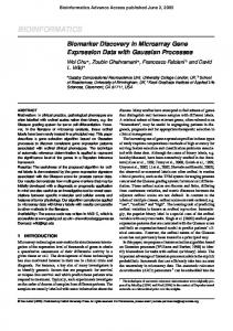
Figure 1.3: A training set for a simple learning problem with one input variable x and one output variable y. The dots represent the observed samples.

Figure 1.4: A second realization of the training set for the same phenomenon observed in Figure 1.3. The dots represent the observed samples. will focus exclusively on this second phase assuming that the preliminary steps have already been performed by the model designer. Suppose that, on the basis of the collected data, we wish to learn the unknown dependency existing between the x variable and the y variable. In practical terms, the knowledge of this dependency could shed light on the observed phenomenon and allow us to predict the value of the output y for a given input (e.g. what is the expected weight of child which is 120cm tall?). What is difficult and tricky in this task is the finiteness and the random nature of data. For instance a second set of observations of the same pair of variables could produce a dataset (Figure 1.4) which is not identical to the one in Figure 1.3 though both originate from the same measurable phenomenon. This simple fact suggest that a simple interpolation of the observed data would not produce an accurate model of the data. The goal of machine learning is to formalize and optimize the procedure which brings from data to model and consequently from data to predictions. A learning procedure can be concisely defined as a search, in a space of possible model configurations, of the model which best represents the phenomenon underlying the data. As a consequence, a learning procedure requires both a search space, where possible solutions may be found, and an assessment criterion which measures the quality of the solutions in order to select the best one. The search space is defined by the designer using a set of nested classes with increasing complexity. For our introductory purposes, it is sufficient to consider here a class as a set of input/output models (e.g. the set of polynomial models)

13

Figure 1.5: Training set and three parametric models which belong to the class of first order polynomials.

Figure 1.6: Training set and three parametric models which belong to the class of second order polynomials. with the same model structure (e.g. second order degree) and the complexity of the class as a measure of the set of input/output mappings which can approximated by the models belonging to the class. Figure 1.5 shows the training set of Figure 1.3 together with three parametric models which belong to the class of first-order polynomials. Figure 1.6 shows the same training set with three parametric models which belongs to the class of secondorder polynomials. The reader could visually decide whether the class of second order models is more adequate or not than the first-order class to model the dataset. At the same time she could guess which among the three plotted models is the one which produces the best fitting. In real high-dimensional settings, however, a visual assessment of the quality of a model is not sufficient. Data-driven quantitative criteria are therefore required. We will assume that the goal of learning is to attain a good statistical generalization. This means that the selected model is expected to return an accurate prediction of the dependent (output) variable when values of the independent (input) variables, which are not part of the training set, are presented. Once the classes of models and the assessment criteria are fixed, the goal of a learning algorithm is to search i) for the best class of models and ii) for the best parametric model within such a class. Any supervised learning algorithm is then made of two nested loops denoted as the structural identification loop and the parametric identification loop. Structural identification is the outer loop which seeks the model structure which is expected to have the best performance. It is composed of a validation phase,

14


which assesses each model structure on the basis of the chosen assessment criterion, and a selection phase which returns the best model structure on the basis of the validation output. Parametric identification is the inner loop which returns the best model for a fixed model structure. We will show that the two procedures are intertwined since the structural identification requires the outcome of the parametric step in order to assess the goodness of a class.

Statistical machine learning On the basis of the previous section we could argue that learning is nothing more than a standard problem of optimization. Unfortunately, reality is far more complex. In fact, because of the finite amount of data and their random nature, there exists a strong correlation between parametric and structural identification steps, which makes non-trivial the problem of assessing and, finally, choosing the prediction model. In fact, the random nature of the data demands a definition of the problem in stochastic terms and the adoption of statistical procedures to choose and assess the quality of a prediction model. In this context a challenging issue is how to determine the class of models more appropriate to our problem. Since the results of a learning procedure is found to be sensitive to the class of models chosen to fit the data, statisticians and machine learning researchers have proposed over the years a number of machine learning algorithms. Well-known examples are linear models, neural networks, local modelling techniques, support vector machines and regression trees. The aim of such learning algorithms, many of which are presented in this book, is to combine high generalization with an effective learning procedure. However, the ambition of this handbook is to present machine learning as a scientific domain which goes beyond the mere collection of computational procedures. Since machine learning is deeply rooted in conventional statistics, any introduction to this topic must include some introductory chapters to the foundations of probability, statistics and estimation theory. At the same time we intend to show that machine learning widens the scope of conventional statistics by focusing on a number of topics often overlooked by statistical literature, like nonlinearity, large dimensionality, adaptivity, optimization and analysis of massive datasets. This manuscript aims to find a good balance between theory and practice by situating most of the theoretical notions in a real context with the help of practical examples and real datasets. All the examples are implemented in the statistical programming language R [101]. For an introduction to R we refer the reader to [33, 117]. This practical connotation is particularly important since machine learning techniques are nowadays more and more embedded in plenty of technological domains, like bioinformatics, robotics, intelligent control, speech and image recognition, multimedia, web and data mining, computational finance, business intelligence.

Outline The outline of the book is as follows. Chapter 2 summarize thes relevant background material in probability. Chapter 3 introduces the parametric approach to parametric estimation and hypothesis testing. Chapter 4 presents some nonparametric alternatives to the parametric techniques discussed in Chapter 3. Chapter 5 introduces supervised learning as the statistical problem of assessing and selecting a hypothesis function on the basis of input/output observations. Chapter 6 reviews the steps which lead from raw observations to a final model. This is a methodological chapter which introduces some algorithmic procedures

1.1. NOTATIONS

15

underlying most of the machine learning techniques. Chapter 7 presents conventional linear approaches to regression and classification. Chapter 8 introduces some machine learning techniques which deal with nonlinear regression and classification tasks. Chapter 9 presents the model averaging approach, a recent and powerful way for obtaining improved generalization accuracy by combining several learning machines. Although the book focuses on supervised learning, some related notions of unsupervised learning and density estimation are given in Appendix A.

1.1

Notations

Throughout this manuscript, boldface denotes random variables and normal font is used for istances (realizations) of random variables. Strictly speaking, one should always distinguish in notation between a random variable and its realization. However, we will adopt this extra notational burden only when the meaning is not clear from the context. As far as variables are concerned, lowercase letters denote scalars or vectors of observables, greek letters denote parameter vectors and uppercase denotes matrices. Uppercase in italics denotes generic sets while uppercase in greek letters denotes sets of parameters.

Generic notation θ θ M [N × n] MT diag[m1 , . . . , mN ] M θˆ ˆ θ τ

Parameter vector. Random parameter vector. Matrix. Dimensionality of a matrix with N rows and n columns. Transpose of the matrix M . Diagonal matrix with diagonal [m1 , . . . , mN ] Random matrix. Estimate of θ. Estimator of θ. Index in an iterative algorithm.

16


Probability Theory notation Ω ω {E} E Prob {E} (Ω, {E}, Prob {·}) Z P (z) F (z) = Prob {z ≤ z} p(z) E[z] R Ex [z] = X z(x, y)p(x)dx Var [z] L(θ) l(θ) lemp (θ)

Set of possible outcomes. Outcome (or elementary event). Set of possible events. Event. Probability of the event E. Probabilistic model of an experiment. Domain of the random variable z. Probability distribution of a discrete random variable z. Also Pz (z). Distribution function of a continuous random variable z. Also Fz (z). Probability density of a continuous r.v.. Also pz (z). Expected value of the random variable z. Expected value of the random variable z averaged over x. Variance of the random variable z. Likelihood of a parameter θ. Log-Likelihood of a parameter θ. Empirical Log-likelihood of a parameter θ.

Learning Theory notation x X ⊂ 0, NE Prob − p ≤ → 1 as N → ∞ N 1 As

Keynes said ”In the long run we are all dead”.

2.1. THE RANDOM MODEL OF UNCERTAINTY

23

Figure 2.1: Fair coin tossing random experiment: evolution of the relative frequency (left) and of the absolute difference between the number of heads and tails (R script freq.R). According to this theorem, the ratio NE /N is close to p in the sense that, for any > 0, the probability that |NE /N − p| ≤ tends to 1 as N → ∞. This results justifies the widespread use of Monte Carlo simulation to solve numerically probability problems. Note that this does NOT mean that NE will be close to N · p. In fact, Prob {NE = N p} ≈ p

1 2πN p(1 − p)

→ 0,

as N → ∞

(2.1.6)

For instance, in a fair coin-tossing game this law does not imply that the absolute difference between the number of heads and tails should oscillate close to zero [113] (Figure 2.1). On the contrary it could happen that the absolute difference keeps growing (though slower than the number of tosses). Script ### script freq.R ### set.seed(1) ## initialization random seed R 0 (n−1)! pz (z) = 0 otherwise Note that • E[z] = nλ−1 , Var [z] = nλ−2 . • it is the distribution of the sum of n i.i.d.2 r.v. having exponential distribution with rate λ. 2 i.i.d.

stands for identically and independently distributed (see also Section 3.1)

42

CHAPTER 2. FOUNDATIONS OF PROBABILITY α zα

0.1 1.282

0.075 1.440

0.05 1.645

0.025 1.967

0.01 2.326

0.005 2.576

0.001 3.090

0.0005 3.291

Table 2.2: Upper critical points for a standard distribution • the exponential distribution is a special case (n = 1) of the gamma distribution.

2.7.4

Normal distribution: the scalar case

A continuous scalar random variable x is said to be normally distributed with parameters µ and σ 2 (written as x ∼ N (µ, σ 2 )) if its probability density function is given by (x−µ)2 1 e− 2σ2 p(x) = √ 2πσ Note that • the normal distribution is also widely known as the Gaussian distribution. • the mean of x is µ; the variance of x is σ 2 . R

• the coefficient in front of the exponential ensures that

X

p(x)dx = 1.

• the probability that an observation x from a normal r.v. is within 2 standard deviations from the mean is 0.95. If µ = 0 and σ 2 = 1 the distribution is defined standard normal. We will denote its distribution function Fz (z) = Φ(z). Given a normal r.v. x ∼ N (µ, σ 2 ), the r.v. z = (x − µ)/σ

(2.7.43)

has a standard normal distribution. Also if z ∼ N (0, 1) then x = µ + σz ∼ N (µ, σ 2 ) If we denote by zα the upper critical points (Definition 4.6) of the standard normal density 1 − α = Prob {z ≤ zα } = F (zα ) = Φ(zα ) the following relations hold zα = Φ−1 (1 − α),

z1−α = −zα ,

1 1−α= √ 2π

Z

zα

e−z

2

/2

dz

−∞

Table 2.2 lists the most commonly used values of zα . In Table 2.3 we list some important relationships holding in the normal case R script The following R code can be used to test the first and the third relation in Table 2.3 by using random sampling and simulation. ### script norm.R ### set.seed(0) N 10. For example, if N = 3 and DN = {a, b, c}, we have 10 different bootstrap sets: {a,b,c},{a,a,b},{a,a,c},{b,b,a},{b,b,c}, {c,c,a},{c,c,b},{a,a,a},{b,b,b},{c,c,c}. Under balanced bootstrap sampling the B bootstrap sets are generated in such a way that each original data point is present exactly B times in the entire collection of bootstrap samples.

4.4.2

Bootstrap estimate of the variance

For each bootstrap dataset D(b) , b = 1, . . . , B, we can define a bootstrap replication θˆ(b) = t(D(b) ) b = 1, . . . , B that is the value of the statistic for the specific bootstrap sample. The bootstrap ˆ through the variance of the set approach computes the variance of the estimator θ ˆ θ(b) , b = 1, . . . , B, given by ˆ = Varbs [θ] 1 This

PB

ˆ

− θˆ(·) )2 (B − 1)

b=1 (θ(b)

where

θˆ(·) =

PB

ˆ

b=1 θ(b)

B

(4.4.7)

term has not the same meaning (though the derivation is similar) as the one used in computer operating systems where bootstrap stands for starting a computer from a set of core instructions

96

CHAPTER 4. NONPARAMETRIC ESTIMATION AND TESTING

Figure 4.1: Bootstrap replications of a dataset and boostrap statistic computation ˆ It can be shown that if θˆ = µ ˆ, then for B → ∞, the bootstrap estimate Varbs [θ] ˆ converges to the variance Var [µ].

4.4.3

Bootstrap estimate of bias

ˆ be the estimator based on the original sample DN and Let θ θˆ(·) =

PB

ˆ

b=1 θ(b)

B

ˆ = E[θ] ˆ − θ, the bootstrap estimate of the bias of the estiSince Bias[θ] ˆ ˆ with θˆ(·) and θ with θ: ˆ mator θ is obtained by replacing E[θ] ˆ = θˆ(·) − θˆ Biasbs [θ] Then, since ˆ − Bias[θ] ˆ θ = E[θ] the bootstrap bias corrected estimate is ˆ = θˆ − (θˆ(·) − θ) ˆ = 2θˆ − θˆ(·) θˆbs = θˆ − Biasbs [θ] R script See R file patch.R for the estimation of bias and variance in the case of the patch data example.

4.5. BOOTSTRAP CONFIDENCE INTERVAL

97

## script patch.R placebo β¯ H

Interval of confidence

Under the assumption of normal distribution, according to (7.1.7) ( ) ˆ − β1 ) p (β 1 Prob −tα/2,N −2 < Sxx < tα/2,N −2 = 1 − α σ ˆ where tα/2,N −2 is the upper α/2 critical point of the T -distribution with N − 2 degrees of freedom. Equivalently we can say that with probability 1 − α, the real parameter β1 is covered by the interval described by s σ ˆ2 βˆ1 ± tα/2,N −2 Sxx is

Similarly from (7.1.5) we obtain that the 100(1 − α)% confidence interval of β0 s 1 x ¯2 + βˆ0 ± tα/2,N −2 σ ˆ N Sxx

7.1.7

Variance of the response

Let ˆ +β ˆ x y ˆ=β 0 1 be the estimator of the regression function value in x. If the linear dependence (7.1.1) holds, we have for a specific x = x0 ˆ ] + E[β ˆ ]x0 = β0 + β1 x0 = E[y|x0 ] E[ˆ y|x0 ] = E[β 0 1 This means that y ˆ is an unbiased estimator of the value of the regression function in x0 . Under the assumption of normal distribution of w, the variance of y ˆ in x0 (x0 − x ¯)2 1 + Var [ˆ y|x0 ] = σ 2 N Sxx PN

x

i . This quantity measures how the prediction y ˆ would vary if where x ¯ = i=1 N repeated data collection from (7.1.1) and least-squares estimations were conducted.

R script Let us consider a data set DN = {xi , yi }i=1,...,N where yi = β0 + β1 xi + wi where β0 and β1 are known and w ∼ N (0, σ 2 ) with σ 2 known. The R script bv.R may be used to: ˆ , β ˆ and • Study experimentally the bias and variance of the estimators β 0 1 ˆ when data are generated according to the linear dependency (7.1.2) with σ β0 = −1, β1 = 1 and σw = 4.

7.1. LINEAR REGRESSION

147

• Compare the experimental values with the theoretical results. • Study experimentally the bias and the variance of the response prediction. • Compare the experimental results with the theoretical ones. ## script bv.R ## Simulated study of bias and variance of estimators of beta_0 and beta_1 in ## univariate linear regression rm(list=ls()) par(ask=TRUE) X