Machine utilizations achieved using balanced FMS ... - Deep Blue

227

III. PRODUCTION PLANNING

Annals of Operations Research 15(1988)229-267

229

M A C H I N E UTILIZATIONS A C H I E V E D U S I N G B A L A N C E D F M S P R O D U C T I O N R A T I O S IN A S I M U L A T E D S E T T I N G

Thomas J. SCHRIBER and Kathryn E. STECKE Graduate School of Business Administration, The Universityof Michigan, Ann Arbor, Michigan 48109-1234, USA

Abstract Stecke [21] has developed mathematical programming approaches for determining, from a set of part type requirements, the production ratios (part types to be produced next, and their proportions) which maximize overall machine utilizations by balancing machine workloads in a flexible manufacturing system (FMS). These mathematical programming (MP) approaches are aggregate in the sense that they do not take into account such things as contention for transportation resources, travel time for work-in-process, contention for machines, finite buffer space, and dispatching rules. In the current study, the sensitivity of machine utilizations to these aggregations is investigated through simulation modeling. For the situation examined, it is found that achieved machine utilizations are a strong function of some of the factors ignored in the MP methodology, ranging from 9.1% to 22.9% less than those theoretically attainable under the mathematical programming assumptions. The 9.1% degradation results from modeling with nonzero work-inprocess travel times (i.e. 2 minutes per transfer) and using only central work-inprocess buffers. Resource levels (e.g. the number of automated guided vehicles; the amount of work-in-process; the number of slack buffers) needed to limit the degradation to 9.1% correspond to FMS operating conditions which are feasible in practice.

Keywords FMS, production ratios, mathematical programming, ievels of detail in modeling, balanced machine workloads, machine utilizations, dispatching rules, simulation.

1.

Introduction

An FMS manager carrying out short-term planning for FMS use is faced with the task of determining, from a set of part type requirements, the subset of part types to be produced next and the proportions in which to produce them. (Other short-term planning tasks faced by the FMS manager are discussed in [20] .) The part types to © J.C. Baltzer AG, Scientific Publishing Company

230

T.J. Schriber and K.E. Stecke, Balanced FMS production ratios

produce next, and the proportions in which to produce these parts, are referred to as a set of production ratios. Stecke [21] has developed mathematical programming (MP)formulations to determine production ratios which maximize overall machine utilization by balancing machine workloads in an FMS. (For the machining resources of which an FMS is composed, overall machine utilization is the average of the individual machine utilizations. Machine workloads are balanced as much as possible relative to a target work. load when the sum of overloads and underloads on machines in the FMS is minimized.) However, these MP formulations only take into account the machining resources of the FMS, and the operation types and times needed to produce each of the required part types. The MP methodology is designed for making aggregate decisions at an early point in the planning phase (see Suri [27] ). The objective of the research reported here is to compare the theoretical overall machine utilization resulting from application of the MP methodology with the machine utilizations actually achieved in a model which more realistically accounts for such additional FMS characteristics as constrained resources for transporting workin-process (WlP), transfer times, limited buffer space, contention for machines, and the rules used to dispatch WIP to machines. In particular, for a hypothesized FMS and a required set of part types, the main objectives are to: (1) determine the level (or alternative levels) of selected non-machining FMS resources needed to achieve theoretical overall machine utilizations when transfer times are realistic; (2) estimate the degradation in overall machine utilizations when there are inadequate nonmachhaing resources; and (3) measure the sensitivity of overall machine utilizations to two alternative WIP dispatching rules. An additional objective is to: (4) measure the influence of two alternative WlP dispatching rules on the average and variance of part type manufacturing times. Common to each of these objectives is the goal of better understanding the underlying reasons for observed behavior by measuring and interpreting such things as the number of transfers of WlP into buffers, the residence time of WIP in buffers, and the fraction of the time that various numbers of buffers are occupied and various numbers of AGVs are in use. Section 2 introduces and discusses the FMS scenario which is investigated here. Section 3 compares the simplifying assumptions made in the mathematical programming solution for such scenarios with some of the characteristics of a realistic FMS. Section 4 discusses the levels of aggregation used in this work, and section 5 explains how the section 2 FMS is interpreted as a flexible flow system for purposes of this study. Section 6 presents the details of the simulation model used for the study, and section 7 comments on model verification. Section 8 discusses the design of the simulation experiments. Section 9 presents and discusses results. Sections 10 and 11, respectively, summarize the work and comment on future research directions. Calculations are then shown in a series of three appendices.


2.

231

The FMS scenario investigated

Assume the machining resources in an FMS consist of 1 mill, 2 drills, and 2 vertical turret lathes (VTLs). Suppose 10 types of parts are to be produced by this FMS, with the various part type machining and production requirements shown in table 1. In run 1 of the production process, the FMS is to be used to build a subset Table 1 Specifications for a particular FMS problem Machining times (minutes) Part type

Mill

Drill

VTL

Total parts ordered

1 2 3 4 5 6 7 8 9 10

10 15 40 30 10 10 20 15 25 5

60 20 10 20 50 30 10 20 10 40

50 40 30 20 20 20 10 30 20 40

60 50 30 30 35 45 15 25 30 50

of the 10 part types. (Run 1 ends when the production requirement for one of the part types in this subset has been met; see below.) The run 1 production ratios are to be determined so that workloads on the three machine types are balanced. Stecke and Kim [23] have presented solutions both to the specific problem stated above, and to several variations on this problem. (Refer to Stecke and Kim [22,24,25] for treatment of the problem of how to operate the FMS after run 1 is finished.) A set of production ratios which balances machine workloads for this problem specifies that part types 2, 5, 6, 8, and 10 are to be built in proportions of 2, 1, 2, 1, and 1 [23]. That is, of every 7 parts built, 2 are to be of type 2; 1 is to be of type 5; 2 are to be of type 6; etc. The theoretical overall run 1 machine utilization corresponding to this set of production ratios (assuming zero WIP transfer time) is 95.2%, and the corresponding theoretical mill, drill, and VTL utilizations are 76.1%, 100%, and 100%, respectively. (The calculations are presented in appendix A.) It is the set of FMS machining resources, the set of part type requirements, and the run 1 production ratios described above which are the basis for the study of overall machine utilization reported here.

232

3.


FMS factors ignored in the MP solution

The mathematical programming solution for the section 2 problem only takes into account the machining resources of the FMS and the part type information in table 1. The solution ignores such secondary FMS resources as the number and types of buffers to provide for work-in-process (WlP). (The types of buffers provided might include central buffers and/or buffers local to machines.) The level of resources used to transfer WlP from point to point in the system is not taken into account, either, in the mathematical programming solution. (Pallets and fixtures, loading and unloading stations, and washing and inspection stations are other secondary FMS resources not mentioned in the section 1 problem statement. As explained further below, however, these secondary resources can be taken into account in the MP solution of the machine balancing problem.) Furthermore, the MP solution ignores such geometric aspects of the FMS as the absolute and relative locations of the various system resources, and the routes for transfer of WlP (such as pathways for automated guided vehicles and/or the placement of conveyors). (The role played by these geometric considerations in FMS design has recently been discussed by Heragu and Kusiak [8] .) Nor does the MP solution take into account such secondary time requirements as the time required to transfer WlP from point to point in the system, or the time required for palletizing, depaUetizing, fixturing, defLxturing, and refixturing parts. The time required to move empty pallets from unloading stations to loading stations is not considered, either. (As explained in section 5, however, such other secondary time requirements as the time needed to wash and/or inspect parts between operations, when such washing and/or inspection is necessary, can be taken into account in the MP formulation.) FMS operating policies are ignored in the mathematical programming solution, too. One such operating policy involves the quantity of WIP permitted in the system. Another is the part input sequence. (That is, when work on a part is finished, what type of part is to be admitted next to take its place? For a given set of production ratios, there are usually many alternative part input sequences which could be specified. There are also many alternative part input sequences even when production ratios are not explicitly specified.) A third type of operating policy not considered in the MP formulation involves the rules used to dispatch work to machines. For example, dispatching rules based on FIFO (first-in, first-out) might be used, or rules based on SPT (shortest processing time) might be used. (More of the specifics of the FIFO-based and SPT-based dispatching rules used in this study are given in detail in section 8.) Potential system operating discontinuities resulting from tool failures, other types of machine breakdowns, and the periodic withdrawal of machines from service for such things as scheduled maintenance, are also not taken directly into account in


233

the MP solution for the workload balancing problem. The possibility of machine substitution is not considered, either. (Machine substitution is the use of one type of machine to accomplish a step normally done by another type of machine. Machine substitution might take place when a preferred type of machine has broken down, or is undergoing periodic maintenance, or is being contended for in the short run by a large number of jobs.) Finally, the mathematical programming solution does not take into account such secondary ]ob characteristics as due dates or lateness penalties. (Note that no due dates or lateness penalties are included in table 1.) Also not considered is the order in which various types of jobs use various types of machines and whether there is any potential flexibility in this order. In conclusion, the MP solution methodology for the workload balancing problem addresses only a subset of the issues involved in the realistic operation of a flexible manufacturing system. This leads to the question of how applicable the MP solution to a given problem will be in more realistic settings. What levels of secondary FMS resources are needed to achieve the overall machine utilizations promised in the MP solution? For a given level of secondary resources, what machine utilizations can be achieved? At what rate does overall machine utilization change with changing levels of secondary resources? And what influences do operating procedures have on the answers to these questions? The purpose of this study is to investigate the answers to such questions for a specific case, with the longer term goal of developing guidelines for answering questions of this type in general. 4.

M o d e l aggregation in this s t u d y

In modeling a system, it is important to determine which factors are to be aggregated or possibly even ignored for the purposes at hand. This section discusses why some of the features of flexible manufacturing systems outlined in section 3 can be ignored in the present study.

Machine breakdowns. If a machine breaks down, this causes the system (and therefore the problem) to change in the sense that the set of machining resources making up the FMS is (temporarily) reduced. The purpose of this study is to investigate machine utilizations achieved for a given set of system resources, prior to possible eventual change in the composition of these resources. Because we want to understand the issues separately, machine breakdowns (or, altematively, the periodic withdrawal of machines from service for preventive maintenance) are not considered in this work. (For a recent study which deals with unreliable machines in an FMS, see Maimon and Gershwin [ 12] .) Due dates. The degree of importance of due dates varies from time to time and from FMS to FMS. Due dates can be of immediate importance .in some cases (e.g. in a demand-driven FMS), and of lesser importance in other eases (e.g. when part

234


type requirements have been specified to maintain inventory levels). For example, many systems are driven by weekly, or even monthly, production requirements. The planning horizon may then allow such systems to be operated with the objective of maximizing overall machine utilization in the shorter term. The periodic requirements may best be met by maximizing overall machine utilization in the shorter term, subject to possible longer term modifications designed to meet periodic due dates. It is assumed in this study that the objective is shorter term maximization of machine utilizations, and so due dates are not considered.

Refixturing of parts. In an FMS, some types of parts may have to leave the system temporarily from time to time to be refixtured. After refixturing, such parts are then reintroduced into the system and additional machining steps are performed on them. It is often possible to treat refixtured parts as new parts being introduced into the system, with the restriction that refixtured parts of a given type must be (re)introduced in ratios identical to those for the pre-refixtured parts of the same type. The refixturing complication can be taken into account in the MP methodology for determining production ratios which balance machine workloads. Because the purpose here is to study the sensitivity of achieved overall machine utilization to non-machining aspects of an FMS, refixturing is not an issue in this work. Washh~g and inspection stations. After each operation (or after a series of operations), an in-process part may visit a washing station to remove chips from the part before it goes .to its next machine or station. In addition, parts may be subject to in-process inspection and/or to inspection when finished. Washing and inspection stations, if present, can be treated as machines both for purposes of this study and in the MP formulations. We do not model these operations in this study. 5.

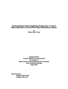
I n t e r p r e t i n g t h e F M S as a flexible f l o w s y s t e m

For purposes of this study, the flexible manufacturing system described in section 1 is interpreted as a Flexible Flow System (FFS). This interpretation is pictured in fig. 1. All part types are assumed to use machines in a unidirectional mill-drill-lathe sequence. No machine type is used by a part type more than one time, and no machines can perform substitute functions. This flexible flow system has the characteristics of an FMS, except that alternative routings are not permitted. In most previous udies of FFSs (e.g. [1,2,9,13,30]), the prodm ion requirements for the part types that will be produced are scaled down to their smallest integer multiples, and these are then used as the production ratios. (Producing in ratios proportional to production requirements defines the machine workloads, which are then almost always unbalanced.) This contrasts with the approach taken here of working with production ratios designed to balance machine workloads. Previous FFS work has often included studying the effect on system performance of alternative choices of part input sequences. In contrast, the work


Raw Material

In

Loading I Station(s)

Finished Goods Out

Empty Pallets and Fixtures Recycle

T T

Station(s)

~L ..... Mills

Drills (2)

(1)

,,,

235

I

121

,,,

1

T ;

Central

(If

Buffers any)

T

Fig. 1. Interpretation of the FMS as an FFS.

here focuses principally on the influence of secondary FMS resources on machine utilization, and does not include investigating how part input sequences for a given set of production ratios affect system performance. The reported FFS studies typically ignore travel time and contention for transportation resources. These two important aspects of a realistic system are explicitly modeled in the current study. As implied in fig. 1, we choose to work only with central buffers here, and do not provide buffers specific to individual machines (or machine groups). There are existing FMSs which onty have central buffers (e.g. the Sundstrand/Caterpillar FMS in Peoria, Illinois [26] ). Some other FFS studies ([24,25]) have also assumed that there are individual machine buffers in the system. In most of the reported FFS studies, however, small buffers of capacity 1 or 2 have been provided between machines. (In one study, however, the system modeled has 30 buffers for 4 machines [1] .) As also implied in fig. 1, no possibility of temporary storage is assumed for fixtured parts, either before the first operation or after the last operation. (Note that if neither loading or unloading is a bottleneck, such temporary storage may not be crucial.)

236

6.


Overall particulars of t h e F F S simulation model

Some important aspects of the simulation model built and used for this study have been described and explained in sections 4 and 5. An overall summary of the characteristics and assumptions of the model is provided below, using categories introduced in section 3.

(1)

Secondaly FMS resources

Automated Guided Vehicles (AGVs) transport work-in-process, with the number of AGVs included as a model parameter. (The term AGV is used here for convenience and to provide vocabulary for later presentation of results and discussion; however, the model is not specific to AGVs as such, but applies for any vehicle- or carrier-based technology.) Only central buffers are provided for work-in.process. The number of buffers is a model parameter. Pallets and fixtures and loading and unloading stations are modeled explicitly, and are model parameters. Fixtures are specific to part types, but pallets are not. (2)

Geometricconsiderations

The geometry of the system is not modeled. This means that neither relative nor absolute locations of loading stations, machines, buffers, or unloading stations are explicitly represented in the model, and the positioning of AGV guidepaths is not taken into account. (3)

Secondary time requirements

Transfer time for work-in-process is a model parameter. As a first approximation, the transfer time between any two points in the system is assumed to be independent of the points involved. Palletizing and depalletizing times, and fixturing and defixturing times, are also model parameters. The time required for empty pallets and fixtures to move between he unloading and loading points is a model parameter. (The model parameter sett.ngs used in this study are given in section 8.4.) (4)

Operatingpolicies

The model provides the user with a choice between either FIFO-based or SPT-based rules for sending WlP to machines.


237

The FIFO-based dispatching rule takes this form: (a) When possible, send WIP to an idle machine from a preceding machine, rather than from a buffer. (In other words, give machine-to-machine transfer precedence over buffer-to-machine transfer. This approach unblocks the preceding machine as soon as possible, and reduces the number of transfers of WIP into buffers.) (b) For machine-to-machine transfer, dispatch that unit of WIP which has been waiting the longest (FIFO) for the now-idle machine. (c) For buffer-to-machine transfer, dispatch that unit of WIP which has been waiting the longest (FIFO) for the now-idle machine. (d) In terms of machine-to-buffer transfer, dispatch that unit of WlP which has been waiting the longest (FIFO) to be moved from the machine at which it is now finished. Note that the dispatching rule described above, although FIFO-based, is not truly FIFO because (a) gives preference to WIP coming from a preceding machine over WIP coming from a buffer. The SPT-based dispatching rule takes this form: (a) If two or more units of WIP are waiting for a machine which has just become idle, dispatch that unit which has the shortest processing time (SPT) on the machine. (No regard is paid to whether the WIP is coming from a preceding machine or from a buffer.) (b) If there is an SPT-tie between WIP at a preceding machine and WIP in a buffer, give priority to the WIP at the preceding machine. (This unblocks the preceding machine as soon as possible and reduces the number of transfers of WIP into buffers.) (c) If there is an SPT-tie between WIP in a common type of location (that is, at preceding machines or in buffers), use first-come, first-served to resolve the tie. The quantity of work-in-process permitted in the system is a model parameter. The part input sequence is also a model parameter. (5)

Operatingdiscontinuities

As explained in section 4, neither machine breakdowns nor the periodic removal of machines from service (such as for routine maintenance) is modeled. Neither breakdowns nor maintenance of equipment used for WIP transfer is modeled, either.

238

(6)


Secondary job characteristics

Neither order due dates nor lateness penalties are specified in the section 1 description of the part type orders on hand, or are recognized in the simulation model as factors to be considered. The rationale for this is given in section 4. 7.

Model c o n s t r u c t i o n and verification

The simulation model, which was built in GPSS/H, version 2 [7,16], was verified (that is, the correctness of the computer code was established) by techniques reported in [17]. These techniques included simulating with a series of increasingly more complicated cases for which model outputs were checked against correct results determined independently by hand, and interactively monitoring the movement of randomly chosen work-in-process as it passed through the system. Interested readers should refer to [17] for more particulars. The model was built and verified by the first author in about seven working days. The model consists of about 150 GPSS blocks, and the model file contains about 425 statements. The computer time required to perform simulations with the model is given in section 8. 8.

Design o f the s i m u l a t i o n e x p e r i m e n t s

The simulation experiments in this study were designed to measure overall machine utilization achieved by the FMS at operating equilibrium for the scenario described in section 2, and to determine (under the section 6 modeling assumptions) the sensitivity of key performance variables to: the number of AGVs, the number of buffers, the WlP level, and the rule used to dispatch parts to machines. The method used to establish conditions of operating equilibrium is explained in section 8.1. The resulting experimental design is presented in section 8.2. Section 8.3 then briefly indicates why a full factorial design was used in this work. Sample size and sample types are discussed in section 8.4, and section 8.5 describes the settings of model parameters for which experiments were performed. 8.1.

ESTABLISHINGOPERATINGEQUILIBRIUM

Operating equilibrium corresponds to a dynamic situation in which measurements, produced by the model, cycle about their average values as the simulation proceeds. All simulated times used in this study (e.g. the machining times specified in table 1 and WIP transfer times) are deterministic, and so there are no variations in model behavior resulting from sampling from probability distributions. (No random number generators were used in the simulation.) The cycling in the values of measurements results from the fact that the part input sequence is cyclic. As pointed out in


239

section 1, the part input sequence is composed of part types 2, 5, 6, 8, and 10 in proportions of 2, 1, 2, 1, and 1, respectively. An input cycle consists then of 7 parts in total (2 + 1 +2 + 1 + 1). The input sequence used in this design, expressed in terms of part type numbers, is 2, 6, 5, 2, 8, 6, and 10. (The chronological order of part introduction is 2, 6, 5, 2, 8, 6, 10; and then 2, 6, 5, 2, 8, 6, and 10 again;etc.)This input sequence was arbitrarily chosen from the potential sequences derived as permutations of the production ratios, except that the repeating part types (types 2 and 6) were nonconsecutive. As stated above, this study is not directed at sequencing and/or scheduling, but considers other FMS influences on machine utilization; as a result, the part input sequence was not varied in the experimental design (however, see section 9.9). In general, an FMS can spend part of its time operating at equilibrium and the rest of its time operating in transition, moving from one set of equilibrium operating conditions toward another. If part type production requirements are large enough, an FMS can reach operating equilibrium; otherwise, for a given set of production ratios, operating equilibrium may not be achieved before the production ratios have to be changed. This study focuses on overall machine utilization during conditions of operating equilibrium, for comparison purposes. It is assumed, then, that production requirements are large enough so that operating equilibrium will be reached and then sustained for some time (see [22,24,25] for studies of FMS behavior when operating during periods of transition). The model as built was devoid of WlP initially. At simulated time zero, parts equal in number to the chosen WlP level, and with no operations yet performed on them, were admitted to the system. Prior to collecting model outputs for purposes of this study, it was then necessary to determine how tong to simulate to arrive at conditions of operating equilibrium. This determination was accomplished experimentally for a number of alternative model settings ~ the following way: (1) After admitting the initialization parts, start the simulation and proceed until an entire 7-part input sequence has been admitted to the model. (2) Suspend the simulation, obtaining output but leaving work-in-process as is. (3) Resume the simulation, proceeding until another 7-part input sequence has been admitted to the model. (4) Suspend the simulation, obtaining output but leaving work-in-process as is. (5) Repeat (3) and (4) a large number of times (e.g. 50 times). (6) Study the pattern of simulated time elapsed between consecutive sets of output. When this pattern begins to cycle (that is, to repeat itself), operating equilibrium has been established. A numeric example will help to clarify this procedure. Consider table 2, which shows a hypothetical time series of simulated time elapsed between consecutive sets

240


Table 2 An exampie of repeating patterns of elapsed simulated time between consecutive output sets Output set

Simulated time (minutes) elapsed since preceding output set was produced

1 2 3 4

110 114 119 116

(transient period)

5 6 7 8 9

120 117 121 114 122

(equilibrium; model cycle 1)

10 11 12 13 14

120 117 121 114 122

(equilibrium; model cycle 2)

15

and so on

of output produced per the above scheme. During the period of model operation corresponding to output sets 1 through 4, transient conditions are in effect. For the next 5 sets of output, the elapsed simulated time between output sets is 120, 117, 121, 114, and 122. This pattern then repeats itself for the following 5 sets of output, and for the 5 sets of output after that (not shown in table 2), ad infinitum. We conclude that in this case, operating equilibrium has set in after only 459 simulated minutes of model operation (459 = 110 + 114 + 119 + 116). The number of output sets produced before operating equilibrium was established was found to depend on the setting of the model parameters (e.g. the number of AGVs, the level of work-in-process, and the number of slack buffers, if any). Among the cases we experimented with, the most extreme case required that 15 output sets be produced before equilibrium was established. (This case involved 3 AGVs, 2 slack buffers, and a WlP level of 7 (see section 9.2).) This corresponded to 1731 minutes of simulated time, or less than four 8-hour shifts. The number of output sets per repeating pattern (that is, per model cycle) at operating equilibrium was also found to depend on the setting of the model parameters. In the most extreme case found, there were 27 output sets per repeating


241

pattern. (This case also involved 3 AGVs, 2 slack buffers, and a WlP level of 7.) This corresponded to 2 896 minutes of simulated time, or slightly more than six 8-hour shifts. Having gained these insights into the duration of transient model operation and the duration of a model cycle under conditions of operating equilibrium, the experimental plan described in the next subsection was devised. 8.2.

EXPERIMENTALDESIGN

For a given setting of model parameters, it would only be necessary to measure the model outputs of interest during one model cycle under conditions of operating equilibrium. However, this approach would require prior experimentation to determine both the duration of transient operation and the duration of a model cycle for each model setting. This approach was impractical because it was labor intensive, and because 240 model settings were involved. Therefore, the following experimental design was used as an alternative: (1) Simulate for twenty-five 8-hour shifts. (2) Suspend the simulation, suppressing output and reinitializing the various statistical accumulators, but leaving work-in-process as is. (3) Resume the simulation for an additional two hundred and fifty 8-hour shifts. (4) Stop the simulation, obtaining output in the process. Step (1) was designed to move well beyond transient model operation and into conditions of operating equilibrium. Step (3) was designed to move through a large number of model cycles (25 or more) at operating equilibrium. Although step (3) likely did not move through an integral number of model cycles, model outputs collected during the large number of simulated cycles would swamp the slightly imbalanced outputs collected during the partial model cycles likely involved at the beginning and the end of step (3). The motivation for this design was to standardize and automate the work. 8.3.

FULLFACTORIALDESIGN

Depending on the WlP level and the number of AGVs in the model, each simulation run, consisting of the four steps described in section 8.2, consumed about 2 CPU seconds on an IBM 3090-400 computer. (It is estimated that the corresponding time required on a PC-AT would be about 1 500 CPU seconds, or 25 minutes.) For the billing algorithm in use at The University of Michigan (where the experiments were performed), this translated into an average cost per run of about U.S.$3.00 during high-rate (daytime) periods, or about 60¢ during low-rate (overnight) periods.

242


Because the simulation costs were modest, especially during low-rate periods, a full factorial design was used in examining the various FMS conditions studied. 8,4.

SAMPLESIZES AND SAMPLEDVARIABLES

For each experimental setting, observations gathered for reporting purposes were recorded by the model under conditions of operating equilibrium for a single simulation consisting of two hundred and fifty 8-hour shifts (see step (4) in section 8.2). For example, overall machine utilization for shift 1, shift 2, shift 3 , . . . , shift 250 was recorded, and then the mean, standard deviation, and frequency class counts (as well as relative and cumulative frequencies) for the resulting sample of size 250 were computed and reported out by the model. (This methodology is known as the method of batch means [i 4] .) Analogous recording and processing of machine utilization by machine type was accomplished by the model. System residence time provides another example of a type of variable observed during each simulation. An observation was made on this variable each time a finished part left the system. The observed value was placed in each of two samples: a sample of system residence times common to all types of parts which the FMS produces (overall system residence times); and a sample of system residence times specific to the type of part. For a simulation of two hundred and fifty 8-hour shifts, the overall residence time sample is much greater than 250 (about 6 250, because about 25 parts are produced per 8-hour shift for the FMS scenario studied here). As in the case of all samples formed by the model, the mean, standard deviation, and frequency class counts (as well as relative and cumulative frequencies) for the resulting residence time samples were computed and reported out by the model. The number of occupied buffers provides an example of yet another type of variable observed during each simulation. An observation was made on this variable at each reading of the simulated clock. Each such observation was made immediately after the clock had been advanced from its previous reading to its new reading. The observed value (weighted by the number of simulated time units through which the clock had been advanced) was placed in a sample of such observations. At the end of the simulation, the mean, standard deviation, and frequency class counts for the resulting sample of occupied buffers were computed and reported out by the model. Machine utilizations, system residence times, and the number of occupied buffers are representative of the types of variables whose values were observed in this study. Other values observed include the number of buffer entries per shift, the timeweighted number of AGVs in use, production rates, fraction of the time that machines were feed-starved, and fraction of the time that machines were output-blocked. More particulars are provided in section 9, along with numbers for selected cases.


8.5.

243

EXPERIMENTALSETTINGS

All experimental results reported here are based on the assumptions that there is no limit to the number of pallets and fixtures; and that palletizing, fixturing, defixturing, and depalletizing are done external to the system (or, equivalently, are done in zero time). In other words, these resources and/or timings were not allowed to be bottlenecks in this study. The time required for an AGV to transport WlP between any two points (e.g. from the loading station to the mill; from one machine to another; from a machine to a buffer; from a buffer to a machine; from a vertical turret lathe to an unloading station) was assumed to be a constant 2 minutes per transfer. This assumed transport time of 2 minutes is the sum of four components: (1) time for the AGV to travel to the sending point (loading station; machine; or buffer); (2) time for the palletized unit of WlP to move onto the AGV; (3) time for the loaded AGV to travel to its destination; and (4) time for the palletized unit of WlP to move off the AGV to its receiving machine, buffer, or unloading station. More details about the handling of travel time in the model are reported in appendix B. An important experimental variable is the quantity o f work-in-process. In this FMS scenario, the minimum quantity of work-in-process of interest is 5 (because there are 5 machines in the system). The logical maximum for this quantity is the minimum of (i) the number of pallets; (ii) the number of fixtures; (iii) the sum of the number of machines and the number of buffers. With no limit assumed for pallets and fixtures, the maximum quantity of WlP in this research equals the sum of the number of machines and the number of buffers. (Each WlP unit must be either at a machine or in a buffer, except during the time interval when it is being transferred from one location to another.) With WlP at its maximum level, there are no slack buffers in the system. (A slack buffer is a buffer not strictly needed to accommodate the quantity of work.inprocess.) With the quantity of WlP set at one or more units below this maximum level, the system has one or more slack buffers. Slack buffers can play a key role by reducing the occurrence of output-blocking at machines. (Output-blocking occurs when WIP cannot be removed from a machine and remains there, tempotarily preventing use of the machine by the next unit of WlP.) Experiments were performed for the cases of 0, I, 2, and 3 slack buffers. In some experiments, the FIFO-based dispatching rule described in section 6 was used. In other experiments, the SPT-based dispatching rule was used. These rules were used under identical scenarios, for comparison purposes. 9.

E x p e r i m e n t a l results

Representative experimental results are presented and discussed in this section. To provide a basis for the discussion, the steps making up a machine cycle are

244

T.J. Schlqber and K.E. Stecke, Balanced FMS production ratios

summarized in section 9.1. The two primary performance measures on which this study focuses, overall machine utilization and system residence time, are then reported and discussed in sections 9.2 and 9.4, respectively. Selected subsidiary performance measures (e.g. the numbers and sources of buffer entries and the fraction of the time that machines are either feed-starved or output-blocked), which provide insights for better understanding the behavior of the primary performance measures, are then presented in additional subsections. 9.1.

THE STEPS MAKINGUP A MACHINECYCLE

In general, a machine cycles repeatedly through the three-phase process of being feed-starved, productively engaged, and output-blocked. (Consistent with assumptions made in this study, the preceding statement ignores the possibility of machine breakdowns.) The particulars of these three phases are spelled out below, using the vocabulary of AGVs and assuming that a system provides only central buffers. (1)

Feed-starved

A machine is feed-starved when it is ready to work but has no work to do. During the feed-starved portion of a cycle, a machine: (a) waits (if necessary) for a next part to need it, (b) then waits (if necessary) for an AGV to become available; (c) and finally waits for the AGV to bring the part to the machine. (2)

Productively engaged The machine is productively engaged ("utilized") while it is machining the part.

(3)

Output-blocked During the output-blocked portion of a cycle, a machine: (a) waits (if necessary) for a destination (a next machine, or a buffer, or an unloading station) to become available for the part on the machine; (b) then waits (if necessary) for an AGV to become available; (c) and finally waits for the AGV to come to the machine and remove the part.

As described above, the feed-starved, productively engaged, and outputblocked parts of a machine cycle are mutually exclusive and collectively exhaustive. Note in particular that the feed-starved part of a cycle does not begin until the outputblocked part of the preceding cycle has ended.


245

The overall machine utilizations corresponding to the fraction of the time machines spend in phase (2) are reported in section 9.2. The fraction of the time machines spend either in phase (1) or phase (3) are given for selected cases in section 9.6. 9.2.

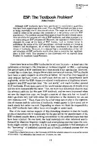
OVERALLMACHINEUTILIZATIONSAND THEIR VARIABILITY

Tables 3 and 4 display information about the overall machine utilizations (expressed as percentages) achieved when the FIFO- and the SPT-based dispatching rules were used, respectively. Each nonparenthesized table entry is the average utilization resulting from one simulation consisting of two hundred and fifty 8-hour shifts under conditions of operating equilibrium (see section 8). (Utilization typically varies from shift to shift because the operating conditions in effect during a shift are undergoing cyclical change.) The parenthesized table entries show the corresponding sample standard deviations. The rows in each of tables 3 and 4 correspond to WlP levels ranging from 5 to 10 in steps of 1. The columns correspond to numbers of AGVs ranging from 1 to 5 in steps of 1. For each WlP/AGV combination, overall machine utilizations are shown for the alternative cases of 0, 1, 2, and 3 slack buffers (see the legend at the bottom of the tables). The theoretical maximum overall machine utilization achievable for all simulations performed in this work is 86.6%. (The calculation is given in appendix B.) If travel time were zero, the theoretical maximum overall machine utilization would be 95.2% for the scenario under study. (Appendix A gives this calculation.) The combination of realistic travel times and the use of only central system buffers consequently degrades the maximum feasible overall machine utilization by 9.1% (or by 8.6 percentage points in absolute terms). For the FIFO-based dispatching rule, table 3 indicates that the 86.6% theoretical maximum overall utilization was not achieved at WlP levels of 5 or 6, but was consistently achieved with 2 and 3 slack buffers when the WlP level was 7 or more and there were at least 4 AGVs. The least complicated operating conditions under which the theoretical maximum overall utilization is achieved in table 3 correspond to a WlP level of 8, 2 AGVs, and 2 slack buffers. These conditions correspond to reasonable levels of resources in an FMS, which means that it is reasonable to expect to achieve maximum machine utilizations in practice. The highlighted cells in table 3 are those for which the maximum overall machine utilization of 86.6% was realized. Note that there are many cells for which the maximum utilization was almost realized. For example, utilizations of 85.8% were realized with 4 or 5 AGVs at a WlP level of 6, and with 2 or 3 slack buffers. It would be tempting to use a t (or z) statistic to make inferences (e.g. confidence intervals; hypothesis testing) both within and between cells in tables 3 and 4. However, this cannot be justified unless the shift-by-shift overall machine

246


Table 3 Means and (standard deviations) of overall machine utilizations with the FIFO-based dispatching rule

N u m b e r of AGV's 1

5

2

3

4

5

73.5 (0.44)

75.6 (0.51)

74.6 (0.38)

78,1 (0.41)

75.8 (0.40)

78.1 (0.46)

75.8 (0.40)

78.1 (0.46)

75.8 (0.40)

78.1 (0.46)

73.0 (0.30)

73.0 (0.30)

79.1 (0,29)

79.1 (0.29)

79.4 (0.27)

79.4 (0.27)

79.4 (0.27)

79.4 (0.27)

79.4 (0.27)

79.4 (0.27)

73.7 (0.57)

77.8 (0.57)

75.2 (0.41)

83.7 (0.07)

75.8 (0.30)

85.1

76.8

85.1

75.8

85.1

(0.20)

(0.29)

(0.21)

(0.29)

(0.21)

78.7 (1.11)

78.7 (1.12)

84.5 (0,40)

84,5 (0.42)

84.7 (0.19)

84.7 (0.19)

85.8 (0.21)

95.8 (0.21)

85.8 (0.21)

85.8 (0.21)

85.2 (0.34)

76.6 (0.43)

85.3 (0,30)

(0.43)

i

6

iiiii

i

i

> ..J

7

8

9

10

74.0 (0,65)

78.1 (0.53)

76.3 (0.47)

81.3 (0.28)

80.0 (0.30)

79.5 (0.40)

85,1 (0.32)

85.2 (0.38)

73,9 (1.29)

78.7 (0.35)

75.2 (0.51)

82.1 (0.17)

78.9

78.9

~6-6~'~ ~ 6 . 6 -'~

~Lo.~.2~

76.5 (0.44)

~86.6TM ~6.6~"~ -f"~86.~/;"~86.6~ (~00.2~

7 6 . 6 "H

85.3 (0.30)

p'-86.6""~ P'~6.6TM

~ 2 ~ ~ 2 ~ . 2 ~ ~ 2 ~ ~:2~

78,2 (0.74)

85.9

(0.49)

78.1

~6.6~¢~

(1.02) ( ~ . 2 ~

7 8 . 1 ~86.6 TM

(1.02) ~ : 2 ~ ,

(0.26)

86.3 ~86 6" ~86.~ ~ 6 6 TM %6.6TM ¢o26) (,Lo1 ~ . 1 ~ ~1~.1~

76.6 (0.54)

86.2 (0.21)

86.3

(o.59)

(0.57)

73.9 (0,56)

77.6 (0.81)

75.2 (0.40)

83.5 (1.32)

78.7 (0.42)

78.8 (1.06)

85.5 (0.43)

85.5 (0.43)

73.4 (0.52)

78.1 (0.37)

77.5 (0,52)

82.8 (1.22)

77.9 ~r86.6~ 77.2 (0.49) ;>%~0.21~.~ (1.08)

79.2 (0,76)

80.6 (0.32)

85.1 (0.50)

86.1 (0.45)

86.1 (0.50)

~'86.~ ~6.~ %((0.21)~:

86.1

(0.39)

75.8 (0.34)

86.0 (0.22)

75.8 (0.31)

86.0 (0.23)

r s 6 . 6 " ~ r 8 6 . 6 ~ ~'~86.6~ ~ 6 . ( ' ~ 85.8 (0.21)

77.2 (1.08) ~ . 2 ~

Pr86.6~ ~,~86.6~ /~86.6~'~ ;~'~86.6~

~1~1~

i

Leg~.~: IIo 213 I~ !I S~ack Buffers

~ 2~.2~


247

Table 4 Means and (standard deviations) of overall machine utilizations with the SPT-based dispatching rule

Number 1

of AGV's

2

3

4

5

,,,,,,,,,

5

6

..I

7

0_

8

75.8 (0.35)

75.5 (0.46)

77,5 (0.37)

7613 (0.49)

78.I (0.46)

76.3 (0.49)

78.1 (0.46)

76.3 (0.49)

78.1 (0.46)

75.8 (0.36)

75.8 (0.36)

7g.1 (0.29)

79.1 (0.29)

79,4 (0.27)

79.4 (0.27}

79.4 (0.27)

79.4 (0.27)

79.4 (0.27)

7g.4 (0,27)

74.6 (0.35)

78.7 (0.38)

81.3 (0,34)

84.4 (0.42)

78.1 (0.54)

84.7 (0.19)

76.3 (0.48)

85.8 (0,21)

78.3 (0.48)

85.8 (0.21)

78.1 (0.37)

78.1 (0.37)

84.5 (0.40)

84.5 (0.31)

84.7 (0.19)

84.7 (0.20)

85.8 (0.21)

85.8 (0.21)

85.8 (0.21)

85.8 (0.21)

74.6 (0.35}

78.7 (0.49)

82.0 (0.25)

85.1 (0.38)

82,3 (0.21)

851

85.1

~ 6 . 6 TM

86.4

823 (0,21)

863 (0.28)

78.1

781

ii N

~ 6 . 6 TM 78.3 ~.23~ (0.48)

(051)

(0.5t)

(o.32) (o.28) ~ 2 ~ ( 0 2 1 )

746 (0.36)

787 (0,38)

(0.25)

78.1 {0.41)

78.1 (0.41)

74,6

78.7

820

~6~ ;.~.20)~

~6.6""~ 85.1 86.3 ~.2~ (0.28)!(0.28) 82.0

85.5

78.1

78.1

85.5

85.1

(0.48)

(0.48)

(0.43)

(0.31)

74.6 (0.35)

78.3 (0.37)

8t.3 (0.34)

86.| (0.46)

I

P~6.6"~ 78.3 ~ 6 . 6 ~ ~,,,~._~0"20)jc,~:;(0.48) ,~(~'20)~.

%66TM ~ 6 ~ %6.6~'~6.6"~ ~:20~2~.2~.2~ 763 (0.50)

~ 6 ~ ~.(~.17)j~,

763 (0.50)

~6~ ~!1~

86.4 ~ 6 - 6 TM ~ 6 . ~ F~6.6~6.~ (0.22) ~ . 1 ~ , . ( ~ , 2 ~ . ~ . 1 ~ . 2 ~

82.3

~ 6 . 6 ~'~

(0.36) (o.38) (0.25) (0.43) 1(0.22) ~ . 2 ~

10

,111ii i

73.5 (0.36)

78.3

~6.~

(o,51) ~ . 1 9 ~

78.3 ~"~6,6~'~ (0.51) ~ . 2 o ) j

~ 6 . 6 TM :; 8 6 . ~

~6.6~

.~886,6 . . . . . . .TM ~ ; ' 8 6 . 6 ~ 6 . ~. . .

~.21)

~.1

~27~., L~.2~,,.21)j,,~

~

78,1 (0.25)

2~

86.1 78.3 (0.39) ( 0 . 6 2 )

7-86.6"~ (~.1~

78.3 ;;~"-86.6~ (0.52) ~.... ' 2 1 ) Z~

~ 6 . 6 TM ~ 8 6 . 6 ~I~ ~ ' 8 8 6 . 6 ~ 6 . 6 ~ ' - 8 6 . ~

78.1

78.1

85.1

85.4

86.1

(0.31)

(0.31)

(0.50)

(0.25)

(0.50)

~.2~

~ : 1 ~ . 1 9 ) ~ . 2 ~ , ! ~

I|

I1 !

Slack

Legeo :

o 2 i 3 |

Buffers

248


utilizations are (approximately) normally distributed. We tested the hypothesis of normality by using UNIFIT [11] to perform Chi-square, Kolmogorov-Smirnov, and the Anderson-Darling tests on the shift-by-shift utilizations for arbitrarily selected cases, but the large values of the resulting test statistics forced strong rejection of the null hypothesis of normality. The simplest operating conditions in table 3 correspond to a WlP level of 5, 1 AGV, and 0 slack buffers (see the uppermost left cell in the table). The overall machine utilization realized under these conditions is 73.5%, which is 84.9% of the theoretical maximum. Hence, the number of AGVs must be increased from 1 to 2, the WlP level from 5 to 8, and the number of slack buffers from 0 to 2, to increase machine utilization by 11.4 percentage points. We conjecture that WlP levels of 5 or 6 are inadequate for achieving the maximum theoretical overall machine utilization because machines are too often feedstarved under these operating conditions (see section 9.7), As table 3 demonstrates, the addition of slack buffers can improve overall machine utilizations. ("More may be better".) With 2 AGVs and at a WlP level of 8, for example, going from 0 to 1 slack buffers improves utilization from 75.2% to 82.1%; and going from 1 to 2 slack buffers improves utilization to the theoretical maximum of 86.6%. We conjecture that this beneficial effect of more slack buffers results from reducing the level of output-blocking at machines (by providing a temporary destination for parts which cannot be transferred immediately from their current machine to their next machine) (see section 9.7). Beyond a certain level, however, additional slack buffers are not useful. ( "More is not necessarily better".) At a WlP level of 6, for example, and for all five alternative AGV cases, going from 2 to 3 slack buffers fails to improve overall machine utilization at all, even though utilization is short of the theoretical maximum for each of these cases. We conjecture that this results because beyond a certain number of slack buffers, feed-starving dominates output-blocking when machine utilizations are below their theoretical maximum. In table 3, increasing the WlP level in some cases results in increased overall machine utilization, other things being equal. (Again, "more may be better".) For example, with 2 AGVs and 2 slack buffers, going from a WlP level of 6 to 7 to 8 results in utilizations increasing, respectively, from 84.5% to 85.1% to 86.6%. We conjecture that this is because feed-starving dominates output-blocking under these conditions, and increasing the WlP level decreases the degree of feed-starving. On the other hand, increasing the WIP level in some of the table 3 cases results in decreased overall machine utilization, other things being equal. ("More may be worse".) For example, with 2 AGVs and 2 slack buffers, going from a WlP level of 8 to 9 to 10 results in utilizations dropping, respectively, from 86.6% to 85.5% to 85.1%. The increased WlP levels reduce the ratio of WlP to slack buffers, and so increases the degree of output-blocking, which we conjecture dominates feed-starving in these cases.


249

In table 3, increasing the number of AGVs results in increased overall machine utilization in most cases, other things being equal. For example, at a WlP level of 7 and with 3 slack buffers, going from 1 to 2 to 3 AGVs results in utilizations increasing, respectively, from 79.5% to 85.2% to 86.6%. We conjecture that output-blocking dominates in these cases, and that its detrimental effect decreases when there are more AGVs to move WlP from machines into buffers. There are almost no cases in table 3 i n which increasing the number of AGVs decreases overall machine utilization, other things being equal. This does happen in going from 2 to 3 AGVs at a WlP level of 8, and with 3 slack buffers. The decrease in utilization is small in this case, from 86.6% to 86.3%. (If AGV paths and contention among AGVs for segments along these paths had been modeled, machine utilization might more often have been found to decrease with an increasing number of AGVs beyond some level.) As in table 3, highlighting is used in table 4 to indicate operating conditions under which the theoretical maximum utilization of 86.6% is achieved. Comparison of tables 3 and 4 indicates that when overall machine utilization is below the maximum, the SPT-based dispatching rule almost always outperforms the FIFO-based rule with respect to the utilization measure. For example, at a WlP level of 7 and with 2 AGVs and 1 slack buffer, overall machine utilization is 85.1% for SPT, but only 81.3% for FIFO. Similarly, at a WlP level of 6 and with 4 AGVs and 0 slack buffers, the utilization is 78.3% for SPT but only 75.8% for FIFO. Also, there are two cases in table 5 where the maximum machine utilization is achieved with only 1 slack buffer (3 AGVs, WlP level 7; and 2 AGVs, WlP level 8) by SPT, but not with FIFO. This demonstrates the potentially important influence of dispatching rules on FMS performance. We observe that the SPT-based dispatching rule reduces the average part-bypart variation in the machining times required by the parts using a given type of machine. For example, the time required by the j t h part to use a drill differs less on average from the time required by the preceding part (to use a drill) under the SPT rule than under the FIFO rule. We conjecture that this reduced variation decreases the amount of output-blocking and feed-starving at the bottleneck machines (drills and VTLs; see appendix A) in this FMS, and so increases overall machine utilization. Table 4 (SPT) shows 32 cases in which the theoretical maximum overall machine utilization was achieved, whereas table 3 (FIFO) shows 26 such cases. Here again, the SPT-based dispatching rule is more successful than the FIFO-based rule. A direct comparison of the operating conditions under which FIFO and/or SPT resulted in 86.6% utilization is given in table 5. As shown there, each WlP/AGV combination resulting in 86.6% utilization with FIFO also resulted in 86.6% utilization with SPT. For eight WlP/AGV combinations, however, SPT achieved 86.6% utilization with only 1 slack buffer (e.g. WlP level 8, and 2 AGVs; WlP level 7 and 3 AGVs), whereas FIFO required at least 2 slack buffers.

250


Table 5 Operating conditions achieving the theoretical maximum overall machine utilizations with the FIFO and SPT-based dispatching rules. Number

1

2

of

AGV's

3

4

SPT ...J

7

"

FIFO SPT

n

FIFO

5

SPT FIFO'" SPT

FIFO SPT

FIFO SPT

FIFO SPT FIFO SPT

SPT FIFO SPT

FIFO SPT

FIFO SPT

FIFO SPT FIFO SPT

i

SPT FIFO SPT

FIFO SPT FIFO SPT

FIFO SPT

SPT FIFO SPT

SPT

FIFO SPT

FIFO SPT

I

FIFO 10

SPT

Legend:

12131

SPT FIFO SPT

Slack

FIFO SPT

ii

FIFO SPT

FIFO SPT

, FIFO SPT

FIFO SPT

Buffers

The same "more may be better", "more is not necessarily better", "more may be worse" observations made about table 3 can be made about table 4. We aggest that table 4 be examined carefully in this regard. The trends in tables 3 and 4 are difficult to quantify in general, or even to rank in general. For example, when overall machine utilization is short of the theoretical maximum, does increasing the WIP level by 1 or the number of AGVs by 1 have the more beneficial effect? The answer depends on the operating conditions assumed. In table 3, for example, assuming a WIP level of 5, 2 AGVs, and 2 slack buffers, adding 1 to the WIP level increases utilization from 79.1% to 84.5% (an improvement of 5.4

T.Z Schriber and K.E. Stecke, Balanced FMS production ratios

251

percentage points), whereas adding an AGV increases utilization from 79.1% to 79.4% (an improvement of only 0.3 percentage points). In this case, adding 1 to the WlP is far more beneficial. On the other hand, when the WlP level is 7 and there is 1 AGV and 2 slack buffers, adding 1 to the WlP level decreases utilization from 80.0% to 78.9%, whereas adding an AGV increases utilization from 80.0% to 85.1%. In this case, adding 1 to the WIP level has a counterproductive effect, whereas adding an AGV has a very productive effect. Situations analogous to those described in the preceding paragraph can be found elsewhere in tables 3 and 4. We conclude that when the overall machine utilization is below the theoretical maximum and there is a shortfall in the WlP level, and in slack buffers, and in the level of transportation resources, or in any two of these three factors, it cannot be stated in general (at this time) which single factor should be improved to obtain the greatest benefit in terms of increased overall machine utilization. (That is, the ranking of the gradients associated with these factors is a function of the conditions of FMS operation.) 9.3.

OVERALLPRODUCTION RATES AND THEIR VARIABILITY

For a given FMS scenario and a set of production ratios, average overall production rate, and average production rates by part type, are proportional to the overall average machine utilizations. This means that average production rates can be derived from the information in tables 3 and 4. Variability in production rates is not easily derived, but of course can be estimated by simulation. The theoretical maximum production rate corresponding to the FMS scenario used in this work is 29.09 parts per 8-hour shift. (Appendix B shows that 115.5 minutes are required under the ideal operating conditions described there to produce the 7 parts making up one input cycle. At this rate, 29.09 parts can be produced per 8-hour shift.) Consistent with the small standard deviations in tables 3 and 4, the standard deviations of part production rates are small, and are similar for all alternative operating conditions studied and for use of either the FIFO- or SPT-based dispatching rule. For example, with 2 AGVs, 2 slack buffers, a WlP level of 8, and the FIFO-based rule, the maximum part production rate of 29.09 parts per hour results, with a standard deviation of 0.76. Under the same operating conditions, but with the SPTbased rule, the maximum part production rate also results, with a standard deviation of 0.70. In general, the standard deviation of part production rates ranges from about 2.5% to 3% of the mean. Individual results are not shown here. 9A.

OVERALLSYSTEMRESIDENCE TIMES AND THEIR VARIABILITY

Tables 6 and 7 show overall WlP system residence times (in minutes) with the FIFO- and SPT-based dispatching rules, respectively. (Overall system residence time is the simple average of the residence times experienced by all parts which moved

252

T.J. Schriber and K.E. Steeke, Balanced FMS production ratios

Table 6 Means and (standard deviations) of overall system residence times with the FIFObased dispatching rule Number 1

5

2

of

AGV's

3

4

5

97.1 (10.6) 97.9 (9.7)

94,5 (10.6) 97,9 (9.7)

95.7 91,4 (10.0) (10.7) 90.4 90,4 ( 8 . 0 ) (8.0)

94.3 (10.0)

91,4 (10,7)

94.3 (10.0)

91.4 (10.7)

94.3 (10.0)

(!0,7)

90.0 (s.o)

90,0 (8.0)

90.0 (9.0)

90,0 (8.0)

90.0 (9.0)

90,0 (8.0)

121.7 (19.7) 108.1 (19.4)

110.2 (23.1) 109.0 (19.4)

114.0 !25.1) 101.4 (11.7)

113.1 (25.3)

100.7 (10.1)

113.1 (25.0)

100.7 (10.1)

113.1 (25.0)

100.7 (10.1)

91,4

i

6

102.4 (10.4) 101,5 (13.2)

101.1

101,1

(14.6)

(14.6)

99.9

99.9

(14.7)

(14.7)

i

•~ > m

..I

7

(1.

8

9

lO

135.2 (35.6)

128.0 (9.1) .........

13t.0 (41.0)

123.0 (8.4)

130.8 (40.9)

117,3 (9.6) 195)~

ii

130.5 (40.8)

125.8

117.5

117,4

(16.9)

(20.1)

(19.2)

(16.4)

~4.~

154.6 (77.6)

145.1 (30.0)

152.0 (60.0)

139.1 (10.9)

146.1

133.1

146.3

(49.1)

(20.0)

(51.0)

125.0

117.3 (9.2)

(34.4) 174.0 (99.4)

165.8 (45.4}

167.8 (95.8)

163.3 (45.0)

163,2 (44.3)

194.7 (118.4}

182.8 (9.3)

184.3 (78.8)

172.5 (40.1)

160.5 (54.9)

177,2 (55,5)

167.8 (33.4)

166.0 (17,6)

149,1 (22:0)

130.5 (40.8)

117,3 (9.2)

146.3

~(~7.9)~

132.8 132.6 ~ 3 2 . ~ 2 . ~

171.0 153.9 (80.0) ( 3 2 , ! ) 150.4 150.4 (22.8) (22.8)

99.8

(14.7)

~5.0~j ~s.o~j, ~L4.9~ ~(4.9~

t44.8 2"132.~ ~132.~ (34.4) ~ 5 ~ 5 . ~

144.8

99.9

(14.7)

ii

169.7 (79.2)

149.5 (18,9)

(51.0)

~5.~

f132.0~82~ 169.7 (79.2)

149.5 (18.9)

~149.s~148.s~ ~ 4 8 . s ~ 4 8 . ~ ~49.~'~9.6~

~2.9~4.~ ~9.01,~9.%~ ~tL3.~3.9~!. 183.5 ~851~ 186.2 188.4 185.2 '61-66.o~ (76.6)

Legend:

~3.~

165.8

166.0

(20.8)

(24.0)

(90.9)

,,~2.7~

(11.7)

12 7) ~

(90.1) ~3.2)j~ ~

4)

|I 02 1I31 I| Slack Buffers

through the model for a given level of FMS resources.) Each nonparenthesized table entry is the average overall system residence time resulting from on, simulation consisting of two hundred and fifty 8-hour shifts under conditions of operating equilibrium. The parenthesized table entries show the sample standard deviations for the corresponding shift-by-shift average residence times. The format of tables 6 and 7 matches that of tables 3 and 4. The table rows correspond to WlP levels ranging from 5 to 10 in steps of 1. The columns correspond to numbers of AGVs ranging from 1 to 5 in steps of I. For each WIP/AGV combination, overall system residence times are shown for the alternative cases of 0, 1,2, and 3 slack buffers.


253

Table 7 Means and (standard deviations) of overall system residence times with the SPTbased dispatching rule Number of AGV's 1

5

97.1 (7.9) 94.3 (7.0)

2

•~ > ¢ .-I

7

8

4

5

94.3 (10•1)

94.6 (13,1)

92.1 (10.8)

93.6 (13•5)

91.4 (10.7)

93.6 (13•5)

91.4 (10•7)

93,6 (13.5)

91.4 (10.7)

94.2 (7.0)

90.0 (8.0)

90.4 (8.0)

90.0 (8.0)

90.0 i8.01

90.0 (8,0)

90.0 (8.0)

90.0 (8.0)

90.0 (8.0)

105.4 (14•3)

101.1 (13•8)

109.7 (20.5)

100.7 113.8)

109.4 (20•4)

101.6 (10.6)

109.4 (20.4)

101.6 (10.6)

101.4

i

i

iii

(18•6)

106.9 (17.8)

t 09.7 (16.4)

109.7

101.4

101.1

101.1

100.0

99.9

99.9

99.9

(16.4)

113.9) =(13.9,,,i

(15.6)

(15.6)

(14.7)

(14.7)

(14.7)

(14.7)

126.0 (22.6)

122.0 (45.1)

121.5 (63.2)

~19.~ ~(~4.~

127.7 (70.5)

~ ~7.2~

127.7 (70.5) ~.~7.2~.

114.9

6

3

134.0 (54.5) 128.0 (28.5)

119.2 (26.5)

129.0 117.9 117.6 ~15.7TM t16.7 ~ 1 5 . ~ 5 . ~ ~T16.~ ~ 1 6 . ~ (28.5) (19.5) (20.01 ...~6.~ (16.3) ~ 5 . 2 2 ~ . 2 ~ ~.22~, ~ 5 . ~ 145.1 139.4 ~ 136.9 134.3 145.9 ~ 3 4 . ~ 145.9 ~36.0~

153.2 [lOO.O)

(54.6)

146.3 (47.7)

i47.71 ~9.7)~.~ (31.3)

(27.9)

172.3 (146.4) t64.6 (67.2)

163.3 (77.4)

156.9 149.8 (128.8) (64.0)

156.2 ~ 164,2 ~ 5 2 ~ 164.2 (187.4) ~ ( 9 5 . ~ (180-0) i~(87•1~ (179.7)~(~7.1)~

164•6

15t.1

161.t

~49~48.5~

~48.~t48.5 ~

(67.2)

(62.4)

(62.4)

~ 7 ~ 8 . ~

.,~4.~L4_9. ~

191.5 (193.0)

182.5 (93.3)

175.7 (172.2)

166.4 (89.5)

182.9 167.8 182.3 ~ 6 7 . 5 ~ 182.3 ~ 6 7 . 5 "~ (235.2) (139.5) (234.4) '1~37.~,,~ ( 2 3 4 . 4 ) ~~137 4

t82.9 (87.7)

182.9 (87.7)

167.9 (81.4)

167.3 (76.3)

(86.5) (~5.4)~,~ (125.1)! (59.3)

146.3 ~ 3 3 • ~

(122.8) .~7.1~..~ (122.8) ~ 5 . ~ , ~

t 3 2 . 3 132.3 '7%2.0 ~32.0TM ~ 3 2 . ~ 3 2 . o ~ (28,5) ~ 0 . ~ ~0.~ ~.(~1.~1.~

134.4

i

9

10

Legend:

165.6 ~ 6 5 ~• (72.9) ~ 6 . ~

~ t 6 5 ~~:~ 65.~ ~ 3 . ~ 8 . ~

Slack

~ 4 8 • ~ 1 4 8 • 5 TM ,,~4.~9.~

~65.0~ ~65.0~ ~66.0)~,

75.8

84.7

O) "J rt

(0.32) 85.1 (0.19)

(0.17) "85.1 (0.19)

75.8 (0.32}

84.7 (0.t6)

85.8 (0.19)

85.8 (0.19)

8

77.2

(0.38) %(,0.18~ /~'-86.6~'~ 86.3 ~.1~ (0.26)

iiii

76,2 (0.59)

~s.1 82.8 I~6.6~, 83.8 (o.42) (o.56) (N.O.l~ (0.06) iiii

9

77.2 (0.39) ~6.~ ~

82.6 (0.13) 86.3 (0.26)

....

Io111

Legend: | 2 [ 3 |

Slack

Buffers

table 4. This difference, although larger, is also fairly small. For both input sequences, SPT outperformed FIFO with respect to this average machine utilization measure. The influence of the part input sequence on system performance should be studied further. There is insufficient evidence presented here to even conjecture on the relative importance of the choice of a part input sequence. 1 0.

Summary and conclusions

This research compares the theoretical overall machine utilizations resulting from the applications of mathematical programming to the machine utilizations achieved using a detailed simulation model. Unlike the MP methodology, the simulation model accounts for FMS characteristics such as constrained resources for transporting work-in-process, transfer times, limited buffer space, contention for machines, and the rtdes used to dispatch WIP to machines. For the specific case investigated here, it has been found that: (1)

Using a set o f production ratios resulting from the application of mathematical programming methodology, the maximum theoretical overall machine

260


utilization (with 2-minute WIP transfer times) of 86.6% can be achieved under relatively realistic FMS operating conditions (that is, in a model which relaxes many of the MP assumptions).

(2)

As well as being realistic,the FMS operating conditions also seem to be feasible, requiring in the two simplest cases only 2 AGVs, a WIP level of 8 (when there are 5 machines), and 4 central buffers; or 3 AGVs, a WIP level of 7, and 3 central buffers.

(3)

The degradation in overall machine utilization attributable to having minimum levels on non-machining FMS resources (1 AGV, a WlP level of 5, and no buffers) is on the order of 15%. (The overall machine utilization drops from a theoretical maximum of 86.6% to an achieved level of 73.5%.)

(4)

When there is a shortfall in overall machine utilization, the change in utilization resulting from increasing the level of a resource is not easily predicted (at this time), even qualitatively. More may be better, but more is not necessarily better, and more may even be somewhat worse. It cannot in general be stated (at this time) which single design parameter should be changed to obtain the greatest benefit in terms of increased utilization.

(5)

On average, overall machine utilization achieved with an SPT-based dispatching rule is somewhat better than that achieved with an FIFO-based dispatching rule. However, the system residence time variance is greater for SPT than for FIFO under many FMS operating conditions. (This result is consistent with other findings reported in the literature.)

11.

Future research

Many aspects of this work, and of work of this type, require further study. For a given set of production ratios, for example, the influence of alternative part input sequences on overall and individual machine utilizations needs to be studied. If an important influence is found, guidelines need to be developed for determining good part input sequences. (Because a set of production ratios developed from the MP methodology balances the machine workloads, it is conjectured that a part input sequence which is any permutation of these would also tend to balance machine workloads over time and achieve relatively good overall machine utilizations.) There is often more than one set of production ratios which balances machine workloads. Further research is needed to determine whether some of these ratios are better than others in the sense of being able to achieve maximum overall machine utilization under simpler operating conditions (e.g. level of transportation resources; WIP levels; number of slack buffers). If important differences are found, then guidelines need to be developed for selecting the best set of production ratios from a list of candidates.


261

When only central buffers are provided, the possibility of reserving some buffers for use by WlP coming from bottleneck machines needs to be investigated. The objective here would be to reduce output-blocking at bottleneck machines, letting them start earlier on their next unit of work. The influence of other dispatching rules on overall machine utilization and variability of WlP residence time needs to be studied. For a given FMS, various alternative scenarios (that is, characteristics of parts in the input sequence) need to be studied to determine the extent to which system performance depends on the scenario itself, apart from such operating conditions as the WlP level, the number of slack buffers, and the level of transportation resources. When overall machine utilization is short of the theoretical maximum for given operating conditions, methods must be developed for predicting whether increasing the WlP level, or increasing the number of slack buffers, or increasing the level of transportation resources, will have the most beneficial effect. Perturbation analysis may be of use in this regard [28]. Another possibility might be to develop regression models for various ranges of operating conditions. The importance of aggregation versus disaggregation in the modeling of FMSs needs to be further assessed. For a given issue or issues, it must be determined which factors outlined in section 3 are important to model, and at which levels of detail, and which can be ignored. Relatively general guidelines must be developed for estimating the impact on FMS performance of such controllable factors as the WlP level, the number of slack buffers, the level of transportation resources, and dispatching rules. Acknowledgements We thank two anonymous referees and the associate editor for their careful reading of this paper, and for insightful comments which improved the paper's form and content. The work of Kathryn E. Stecke was supported in part by a summer research grant from the Graduate School of Business Administration at The University of Michigan.

262


Appendix A CALCULATIONOF THE THEORETICALMAXIMUMOVERALLMACHINE UTILIZATION FOR THE FMS SCENARIO IN SECTION 2

(Basis: zero travel time) Table A.1 shows the individual and total machining requirements, by machine type, of the parts making up one input cycle for the set of production ratios used in this study and discussed in section 2. As indicated in the table, each drill and each VTL must be used for 105 machining minutes per input cycle, whereas the mill must be used for 80 minutes. Table A.1 Machining requirements per part input cycle Machining time per part (minutes) Part type

Mill

Drill

VTL

2 5 6 8 10

15 10 10 15 5

20 50 30 20 40

40 20 20 30 40

No. of parts per input cycle

Machining time per input cycle (minutes) Mill

Drill

VTL

30 10 20 15 5

40 50 60 20 40

80 20 40 30 40

Total for all machines of each type:

80

210

210

Total per machine of each type:

80

105

105

2 1 2 1 1

For the table A.1 scenario, the drills and VTLs are bottleneck machines. (Bottleneck machines are ones which must be used to the greatest extent in producing the sets of parts making up an input cycle. For the scenario at hand, the bottleneck machine type is tied between drills and VTLs.) In contrast, the mill is a slack machine. (Slack machines are ones which have more capacity than is needed to produce the set of parts making up an input cycle.) Now assume the following idealized operating conditions are in effect: (1)

A bottleneck machine never has to wait for a part to need it.

(2)

A slack machine never has to wait counterproductively for a part to need it. (Within certain limits, a slack machine can wait in a non-counterproductive fashion for a part to need it, because slack machine utilization will be less than 100% anyway.)


263

(3)

WlP being taken to or from a bottleneck machine never has to wait to get the AGV needed to perform the transfer. (This is equivalent to assuming an unlimited number of AGVs in the system.)

(4)

WlP being taken to or from a slack machine never has to wait counterproductively to get the AGV needed to perform the transfer.

(5)

WIP travel time is zero. (That is, AGVs move instantaneously from point to point.)

Under these ideal conditions, and consistent with the information in table A.1, the 7 parts making up one input cycle can be manufactured in 105 minutes. The number of machining minutes achieved in 105 minutes is 500 (500 = 80 +2 x 105 +2 x 105). During these 105 minutes, the bottleneck machines (the 2 drills and 2 VTLs) will be 100% utilized, but there will be a 25 minute shortfall in use of the mill, which is the slack machine. (The mill's utilization will be 80/105=0.761, or 76.1%.) Of the potential 525 machining minutes (525 = 5 × 105) in a 105 minute time interval, then, only 500 machining minutes will be achieved. This results in an overall machine utilization of 0.952 ( 0 9 5 2 = 500/525), or 95.2%. Appendix B CALCULATION OF THE THEORETICAL MAXIMUMOVERALL MACHINE UTILIZATION FOR THE FMS SCENARIO IN SECTION 2

(Basis: 2 minute travel time) In calculating the theoretically achievable maximum overall machine utilization when travel time is non-zero, assumptions (1) through (4) of appendix A are in effect, but the zero travel time assumption (assumption (5) of appendix A) is eliminated. This study assumes that in transferring a part from one point (the sending point) to another (the destination), it takes 1 minute for an empty AGV to move to the sending point and pick up the part, and then takes 1 more minute for the loaded AGV to move from the part's sending point to its destination and unload the part there. The total time required for a unit of WlP to move between any two points in the system is then 2 minutes. When a bottleneck machine finishes working on a part, the machine becomes idle and remains idle for 1 minute under assumption (3) of appendix A, while the finished part is cleared from the machine. This is "from-time". The machine then remains idle for 2 more minutes under assumptions (1) and (3) of appendix A, while an AGV fetches the machine's next part and brings that part to the machine. This is "to-time" In the model used in this study, no provision is made to overlap "to-time" and "from-time", and there are no local machine buffers. This means that even under

264


the otherwise ideal assumptions (1) through (4), there are 3 minutes of enforced machine idleness per machine operation. Table B.1 repeats table A.1 by showing the individual and total machining requirements, by machine type, of the parts making up one input cycle for the sets of production ratios used in this study and discussed in section 2. Table B.1 also indicates the 1 minute "from-time" and the 2 minute "to-time" which is part of each machine use. Table B.1 Machining requirements and travel times per part input cycle

Part

Machining time plus to-and-from travel time per part (minutes)

type

Mill

Drill

VTL

No. of parts per input cycle

2 5 6 8 10

15+3 10+3 10+3 15+3 5+3

20+3 50+3 30+3 20+3 40+3

40+3 20+3 20+3 30+3 40+3

2 1 2 1 1

Total for all machines of each type: Total per machine of each type:

Machining time plus to-and-from travel time per input cycle (minutes) Mill

Drill

VTL

30+6 10+3 20+6 15+3 5+3

40+6 50+3 60+6 20+3 40+3

80+6 20+3 40+6 30+3 40+3

80 + 21

210 + 21

210 + 21

101

115.5

115.5

Under the above assumptions, table B.1 indicates that the 7 parts making up one input cycle can be manufactured in 115.5 minutes. The number of machining minutes achieved during these 115.5 minutes is 500 (500 = 80 +2 x 105 + 2 x 105). Of the potential 577.5 machining minutes (577.5 = 5 x 115.5) available in a 115.5 minute time interval, then, only 500 machining minutes would be achieved. This results in an overall machine utilization under these assumptions of 0.8658 (0.8658 = 500/577.5), or 86.6% (as used in tables 1 and 2). Corresponding utilizations for each of the machine types would be 0.693 (or 69.3%) for the mill (0.693 = 80/115.5); and 0.909 (or 90.9%) for the drills and VTLs (0.909 = 105/I 15.5).


265

Appendix C CALCULATION OF THE THEORETICAL MINIMUMOVERALL SYSTEM RESIDENCE TIME FOR THE FMS SCENARIO IN SECTION 2

(Basis: 2 minute travel time) The overall system residence time is the average time in the system per part, with the average taken over the 7 parts making up an input cycle. The theoretical minimum overall system residence time is the overall system residence time realized when assumptions (1) through (4) of appendix A are in effect, and when the 2 minute travel time assumption of appendix B is in effect. Table C.1 Individual step times and minimum system residence time (minutes) by part type Part type Step type

2

5

6

8

10

Transport Mill Transport Drill Transport VTL Transport

2 15 2 20 2 40 2

2 10 2 50 2 20 2

2 10 2 30 2 20 2

2 15 2 20 2 30 2

2 5 2 20 2 40 2

Total

83

88

68

73

93

Table C.1 shows the individual step times and resulting minimum total time in the system (labeled "Total" in table C.1) for each type of part which moves through the system, by part type. The average of these minimum in-system times, with the average taken over the 7 parts making up an input cycle, is 79.4 minutes.

266


References [ 1] [2] [3] [4] [5] [6] [7] [8] [9] [10] [11] [12] [13]

[ 14] [15] [16] [17]

[18]

[19] [20] [21]

[22]

R. Akella, Y. Choong and S.B. Gershwin, Real-time production scheduling of an automated cardline, Ann. Oper. Res. 3(1985)403. P. Afentakis, Maximum throughput in flexible manufacturing systems, Proc. 2nd ORSA/ TIMS Conf. on Flexible Manufactun'ng Systems (Elsevier, Amsterdam, 1986) p. 509. M. Berrada and K.E. Stecke, A branch and bound approach for machine load balancing in flexible manufacturing systems, Manag. Sci. 32, 10(1986)1316. R.W. Conway, W.L. Maxwell and L.W. Miller, Theory of Scheduling (Addison-Wesley, Reading, MA, 1967). J. Erschler, D. Ldv~que and F. RoubeUat, Periodic loading of flexible manufacturing systems, Proc. IFIP CongressAPMS (Bordeaux, France, 1982). S. French, Sequencing and Scheduling (Ellis Harwood Ltd., Chichester, England, 1972). J.O. Henriksen and R.C. Crain, GPSS/H User's Manual, 3rd ed. (Wolverine Software Corporation, Annandale, VA, 1988). S.S. Heragu and A. Kusiak, Machine layout problem in flexible manufacturing systems, Oper. Res. 36, 2(1988)258. K.L. Hitz, Scheduling of flexible flow shops - II, Report LIDS-FR-1049, Laboratory of Information and Decision Systems, MIT, Cambridge, MA (1980). A. Kusiak, The part families problem in flexible manufacturing systems, Ann. Opel Res. 3(1985)279. A.M. Law and S.G. Vincent, UNIFIT User's Manual (Simulation Software and Analysis, Tucson, AZ, 1986). O.Z. Maimon and S.B. Gershwin, Dynamic scheduling and routing for flexible manufacturing systems that have unreliable machines, Oper. Res. 36, 2(1988)279. M.L. Pinedo, B. Wolf and S.T. McCormick, Sequencing in a flexible assembly line with blocking to minimize cycle time, Proc. 2nd ORSA/TIMS Conf. on Flexible Manufacturing Systems (Elsevier, Amsterdam, 1986) p. 499. B. Schmeiser, Batch size effects in the analysis of simulation output, Oper. Res. 30, 3(1982) 556. T.J. Schriber, Simulation Using GPSS (Wiley, New York, 1974). T.J. Schriber, A GPSS/H model for a hypothetical flexible manufacturing system, Ann. Opel Res. 3(1985)171. T.J. Schriber and K.E. Stecke, Machine utilizations achieved using balanced FMS production ratios in a simulated setting, Working Paper 486, Graduate School of Business, The University of Michigan, Ann Arbor, MI (1986). T.J. Schriber and K.E. Stecke, Using mathematical programming and simulation to study FMS machine utilizations, Proc. 1987 14h'nter Simulation Conf. (Society for Computer Simulation, San Diego, CA, 1987) p. 725. J.G. Shanthikumar and K.E. Stecke, Reducing work-in-process inventory in certain classes of flexible manufacturing systems, Eur. J. Oper. Res. 26(1986)266. K.E. Stecke, Design, planning, scheduling, and control problems of flexible manufacturing systems, Ann. Oper. Res. 3(1985)3. K.E. Stecke, Procedures to determine both appropriate production ratios and minimum inventory requirements to maintain these ratios in flexible manufacturing systems, Working Paper 448, Graduate School of Business, The University of Michigan, Ann Arbor, MI (1988). K.E. Stecke and I. Kim, A flexible approach to implementing the short-term FMS planning function, Proc. 2nd ORSA/TIMS Conf. on Flexible Manufacturing Systems (Elsevier, Amsterdam, 1986).

T.J. Sch~qber and K.E. Stecke, Balanced FMS production ratios

267

[23 ] K.E. Stecke and I. Kim, Decision aids for FMS part type selection using aggregate production ratios to study pooled machines of unequal sizes, Working Paper 478, Graduate School of Business, The University of Michigan, Ann Arbor, MI (1986). [24] K.E. Stecke and I. Kim, A study of unbalancing and balancing for systems of pooled machines of unequal sizes, Proc. IEEERobotics and Automation Conf. (Raleigh, NC, 1987). [25] K.E. Stecke and I. Kim, A study of FMS part type selection approaches for short-term production planning, Int. J. FMS 1, 1(1988). [26] K.E. Stecke and J.J. Solberg, Loading and control policies for a flexible manufacturing system, Int. J. Prod. Res. 19, 5(1981)481. [27] R. Suri, An overview of evaluative models for flexible manufacturing systems, Ann. Oper. Res. 3(1985)13. [28] R. Suri and J.W. Dine, A technique for on-line sensitivity analysis of flexible manufacturing systems, Ann. Oper. Res. 3(1985)381. [29] C.K. Whitney and T.S. Gaul, Sequential decision procedures for batching and balancing in FMSs, Ann. Oper. Res. 3(1985)301. [30] R.J. Wittrock, Scheduling algorithms for flexible flow lines, IBM Journal of Research and Development 29, 4(1985)401.

Machine utilizations achieved using balanced FMS ... - Deep Blue

Machine utilizations achieved using balanced FMS ... - Deep Blue

Suggest Documents

Machine utilizations achieved using balanced FMS ... - Deep Blue

Constraint Violation Stabilization Using Gradient ... - Deep Blue

ENHANCEMENT OF BOILING SURFACES USING ... - Deep Blue

ENHANCEMENT OF BOILING SURFACES USING ... - Deep Blue

Monitoring Shorebird Habitat Using Softcopy ... - Deep Blue

Deep Unsupervised Clustering Using Mixture of ... - Deep Blue

Scheduling operations on parallel machine tools - Deep Blue

observations on western european machine tool research - Deep Blue

Machine Learning for Flow Cytometry Data Analysis - Deep Blue

Machine Learning for Flow Cytometry Data Analysis - Deep Blue

Supporting Information - Deep Blue

Digital Cookbooks - Deep Blue

ESP:TheTextbookProblem* - Deep Blue

+r - Deep Blue

Untitled - Deep Blue

Untitled - Deep Blue

Tragion - Deep Blue

letters - Deep Blue

Untitled - Deep Blue

Ethnic ... - Deep Blue

Untitled - Deep Blue

Untitled - Deep Blue

Pergamon - Deep Blue

Qualitative Research - Deep Blue