Macroscopic Quantum Models With and Without Collisions - ASC

Macroscopic Quantum Models With and Without Collisions Ansgar J¨ ungel and Josipa-Pina Miliˇ si´ c Institut f¨ ur Mathematik, Johannes Gutenberg-Universit¨at Mainz, Staudingerweg 9, 55099 Mainz, Germany, e-mail: {juengel,milisic}@mathematik.uni-mainz.de

Abstract Recent progress on the derivation of macroscopic quantum models is reviewed. The first part of the survey is concerned with collisionless models, namely quantum hydrodynamic equations. These models are derived from the mixed-state Schr¨odinger system or from the Wigner equation. In the second part, starting from a Wigner-Boltzmann-type equation, quantum diffusion models like the viscous quantum hydrodynamic and the quantum drift-diffusion equations are derived. For these quantum diffusion models, new numerical results for a simple resonant tunneling diode are presented. Moreover, some hybrid macroscopicmicroscopic models are reviewed.

Keywords. Quantum hydrodynamic equations, quantum drift-diffusion equations, moment method, semiconductors, viscosity, hybrid models, resonant tunneling diode. Acknowlegdements. The authors acknowledge partial support from the Project “Hyperbolic and Kinetic Equations” of the European Union, grant HPRN-CT-2002-00282, and from the Deutsche Forschungsgemeinschaft, grants JU 359/3 (Gerhard Hess Award) and JU 359/5 (Priority Program “Multi-Scale Problems”)

1

1

Introduction

The success of the computer industry relies on the miniaturization of semiconductor devices. In order to produce such devices at low cost and to save production time, efficient computer simulations are necessary. As the characteristic dimensions of modern devices are nowadays much smaller than 100nm, the physical models should include quantum mechanical approaches. However, the simulation of semiconductors using microscopic models, like the Schr¨odinger or Wigner equation, is numerically very time consuming. In the literature, macroscopic quantum models have been proposed [2, 37, 44] which seem to represent a compromise between the two contradicting requirements of physical accuracy and computational efficiency. Roughly speaking, these models belong either to the class of quantum hydrodynamic equations or to the class of quantum drift-diffusion models. Also quantum energy-transport equations have been derived [29] but we do not discuss these models here since their properties have still to be studied. The zero-temperature quantum hydrodynamic model consists of the (dimensionless) equations µ ¶ µ √ ¶ J ⊗J ε2 ∆ n ∂t n − divJ = 0, ∂t J − div + n∇V + n∇ √ = 0, n 2 n λ2 ∆V = n − C(x), x ∈ Rd , t > 0, together with initial conditions for n and J. Here, the unknowns are the electron density n(x, t), the electron current density J(x, t), and the electrostatic potential V (x, t). The parameters are the (scaled) Planck constant ε and the Debye length λ. The doping profile C(x) models charged fixed background ions in the semiconductor device. The matrix J ⊗ J consists of the elements Ji Jk , i, k = 1, . . . , d. We refer to, e.g., [9, 18, 86] for textbooks on semiconductor physics. The above equations are the quantum analogue of the zero-temperature Euler equations under an electric force. The quantum term can be √ interpreted √ either as an internal self-potential, the so-called Bohm potential, ∆ n/ n, or as a non-diagonal pressure tensor, (∇⊗∇) log n. Formally, the above equations are equivalent to the Schr¨odinger equation. They are also referred to as the Madelung equations [75], used in plasma physics [73, 74]. The equivalence will be made more precise in section 2.1. Temperature terms can be obtained from a mixed-state Schr¨odinger system or from the Wigner equation via the moment method. We refer to sections 2.2 and 2.3 for details. When using the moment method, the moment equations have to be closed. Typical closures are given by imposing a condition on the heat flux [44] or the temperature [50]. Recently, the quantum moment

2

equations have been closed by extending Levermore’s entropy minimization principle [31]. We review this method in section 2.4. The common feature of the above models is that they do not describe collisions of the electrons with phonons of the semiconductor lattice or with other particles. In fact, there is no complete quantum collision theory up to now. There are many derivations of collision operators modeling the interaction of electrons with phonons [6, 10, 30, 36, 39], but none of them lead to a form which is computationally tractable and, on the same time, is usable for fluid approximations. Moreover, the quantum thermal equilibrium distribution function, which is a Maxwellian in the classical case, is much more complicate [46]. However, some simple collision models have been derived in the literature. For instance, Caldeira and Leggett [22] derived a Wigner-Fokker-Planck equation in the large-temperature limit, describing the interaction of the electrons with a heat bath of oscillators (modeling the semiconductor lattice). Applying the moment method to the Wigner-Fokker-Planck equation, we arrive to a quantum hydrodynamic model containing viscous terms [53, 67]. This so-called viscous quantum hydrodynamic model will be studied in section 3.1. Another simple collision operator is given by a BGK approach (Bhatnagar, Gross, Krook [15]; see (28)). From the corresponding Wigner-BGK equation, in the diffusion limit, quantum drift-diffusion equations can be derived [29]. In the O(ε2 ) approximation, these equations read as follows: µ √ ¶ ε2 ∆ n ∂t n − divJ = 0, J = − n∇ √ + T ∇n − n∇V, x ∈ R3 , t > 0, 6 n with an initial condition for n and coupled to the Poisson equation for V . Here, T is the constant lattice temperature. Another derivation of this model starts from the quantum hydrodynamic equations including a momentum relaxationtime term. Performing the limit of vanishing relaxation time in the diffusively scaled equations, we also obtain the quantum drift-diffusion model. It will be studied in detail in section 3.2. In sections 3.1 and 3.2 we present some new numerical results for a onedimensional resonant tunneling diode using the viscous quantum hydrodynamic and the quantum drift-diffusion models. Recently, hybrid quantum models including collisional effects have been derived. The idea of these models is that in regions where quantum effects are expected to be dominant, highly accurate models are used, whereas in the remaining regions, simpler (diffusion) models are employed. For instance, the mixed-state Schr¨odinger system is coupled to classical drift-diffusion or quantum drift-diffusion models [28, 34]. Collisional effects in the Schr¨odinger part have been modeled via the Pauli master equation [11]. These models are reviewed in section 3.3.

3

2

Macroscopic models without collisions

In this section we derive various versions of quantum hydrodynamic models, either from the Schr¨odinger or the Wigner equation.

2.1

Zero-temperature models

The evolution of a single electron is governed by the (dimensionless) Schr¨odinger equation for the wave function ψ, ε2 ∆ψ − V ψ, x ∈ Rd , t > 0, 2 ψ(0, x) = ψI (x), x ∈ Rd . iε∂t ψ = −

(1) (2)

We assume that the initial datum is given by the WKB state (Wentzel [87], Kramers [70], Brillouin [19]) √ ψI = nI exp(iSI /ε). (3) Then a simple p computation [48] shows that the solution of (1)-(3) is given by ψ(t, x) = n(t, x) exp(iS(t, x)/ε), where (n, S) is a solution of the zero-temperature quantum hydrodynamic equations

∂t J − div

µ

J ⊗J n

¶

∂t n − divJ = 0, µ √ ¶ ε ∆ n + n∇V + n∇ √ = 0, 2 n 2

(4) x ∈ Rd , t > 0, (5)

with the current density J = −n∇S and the initial conditions n(x, 0) = nI (x),

J(x, 0) = −nI (x)∇SI (x),

x ∈ Rd .

The system (4)-(5) is the quantum analogue of the classical pressureless Euler equations of gas dynamics. In the classical limit ε → 0, (4)-(5) reduce to the classical equations. Notice that this derivation requires an irrotational initial velocity. In physics textbooks, often the flow equations √ ε2 ∆ n 1 2 √ =0 ∂t n + div(n∇S) = 0, ∂t S + |∇S| − V − 2 2 n are derived instead of the formulation (4)-(5). In fact, (5) is obtained from the second equation of the above system after spatial differentiation and multiplication by n. The above system also occurs in the derivation of quantum-classical equations for molecular dynamics [20]. It has the disadvantage that it is not defined if vacuum n = 0 occurs. Then the phase S is not defined and the 4

Bohm potential becomes singular. As shown in [48], the formulation (4)-(5) has in general better properties due to the multiplication with the density n. We remark that this derivation has been recently extended to a two-band quantum hydrodynamic model in [1]. The quantum hydrodynamic model is derived for a single particle and therefore, it does not contain a temperature term. In order to include temperature, many-particle systems need to be studied. For such systems, quantum hydrodynamics is not so well established. The starting point is a statistical mixture of particles each of which is described by a single-state quantum hydrodynamic system. Then averaged quantities over the ensemble of quantum states are needed. This leads to a closure problem, also occuring in the passage from kinetic to classical hydrodynamic equations. In the literature, several closure assumptions have been proposed, for instance, small-temperature asymptotics, use of the Fourier law, or entropy minimization. In the following sections, we review these closure strategies in detail.

2.2

Small-temperature models

In the previous section we have derived a relation between the Schr¨odinger and the fluid dynamical picture. Another point of view is given by the Wigner formalism. More precisely, let ψ be a solution of the Schr¨odinger equation (1)-(2) and let ρ(r, s, t) = ψ(r, t)ψ(s, t), where ψ is the complex conjugate of ψ, denote the so-called density matrix. A computation shows that it satisfies the Heisenberg (or von Neumann) equation iε∂t ρ = −

ε2 (∆s − ∆r )ρ − (V (s, t) − V (r, t))ρ, 2

r, s ∈ Rd , t > 0,

(6)

with the initial condition ρ(r, s, 0) = ψI (r)ψI (s). Let w(x, v, t) be the Fourier transform of the density matrix in the variables r = x + εη/2, s = x − εη/2, Z ³ ε ε ´ iη·v 1 w(x, v, t) = ρ x + η, x − η, t e dη, x, v ∈ Rd , t ∈ R. d (2π) Rd 2 2 Then, Fourier transforming the Heisenberg equation for the density matrix (which is equivalent to the Schr¨odinger equation (1)), we obtain the (oneparticle) Wigner equation ∂t w + v · ∇x w + Θ[V ]w = 0, x, v ∈ Rd , t > 0, w(x, v, 0) = wI (x, v), x, v ∈ Rd ,

5

(7) (8)

where Θ[V ] is a pseudo-differential operator [83] defined by Z Z ³ 1 ε ´ ε ´i ih ³ (Θ[V ]w)(x, v, t) = V x + η, t − V x − η, t (2π)d Rd Rd ε 2 2 0

× w(x, v 0 , t)eiη·(v−v ) dv 0 dη.

(9)

We refer to [76] for details of the computation. In order to derive a quantum hydrodynamic model, we prescribe the initial density matrix ¶ µ θ|r − s|2 , r, s ∈ Rd , ρI (r, s) = ψI (r)ψI (s) exp − 2ε2 p where ψI (x) = nI (x) exp(iSI (x)/ε) and θ is the initial temperature. Notice that the initial Wigner function corresponding to this density matrix equals Z ³ ε ´ iη·v−θ|η|2 /2 1 ε ´ ³ η ψ η e dη. ψ x − wI (x, v) = x + I I (2π)d Rd 2 2 Elementary but lengthy calculations give the moments Z wI dv = nI , Rd Z vwI dv = nI ∇SI , Rd Z 1 ε2 (v ⊗ v)wI dv = nI ∇SI ⊗ ∇SI + nI θ Id − nI (∇ ⊗ ∇) ln nI , 2 Rd 4 where Id denotes the identity matrix in Rd×d . Now multiply the Wigner equation (7) by 1, v and 21 (v ⊗ v), integrate over v ∈ Rd and integrate by parts. We introduce, as in the classical case, the particle, current and energy density, respectively, by Z Z Z 1 n= wdv, J = − (v ⊗ v)wdv, vwdv, E = 2 Rd Rd Rd and define, motivated by the above moments of wI , the temperature tensor T via ¶ µ ε2 1 J ⊗J + nT − n(∇ ⊗ ∇) ln n . (10) E= 2 n 4 It can be shown that T is of the order of θ. Then we obtain the quantum

6

hydrodynamic equations with temperature [49], ∂t n − divJ = 0, x ∈ Rd , t > 0, (11) ¶ µ √ ¶ µ 2 ε ∆ n J ⊗J = 0, (12) + nT + n∇V + n∇ √ ∂t J − div n 2 n · ´¸ J` 1 ε2 ³ 2 2 ∂t Ejk − ∂x` Ejk + (Jj T`k + Jk Tj` ) − Jj ∂xk x` ln n + Jk ∂xj x` ln n n 2 8 1 + (Jj ∂xk V + Jk ∂xj V ) + ∂x` qjk` = 0, (13) 2 where the heat flux tensor q is defined by Z (vj − uj )(vk − uk )(v` − u` )w(x, v, t)dv, qjk` =

j, k, ` = 1, . . . , d,

Rd

and u = −J/n is the mean velocity of the particles. Initial conditions for n, J, and E need to be prescribed. Again, the above system of equations has to be closed, i.e., we have to find an expression for q depending only on n, J or T (and their derivatives). The quantum hydrodynamic equations of Gardner [44] are obtained by replacing q in the above energy equation (13) by µ ¶ ε2 2 J` cl qjk` = − n∂xj xk . (14) 8 n However, this closure condition is not asymptotically correct for θ → 0 since the difference q − q cl = O(θ) can be seen to be of the same order as T = O(θ). This difficulty can be overcome by assuming initial states √“almost coherent” √ ε,θ ε,θ 2 ψI = nI exp(iSI /ε) with SI = SI + O( θ) + O(ε ) as θ → 0, ε → 0. Then it can be shown [49] that √ the energy equation (13) holds with q replaced by q cl up to order O(θ) + O( θε2 ) + O(ε4 ). We stress the fact that this quantum hydrodynamic model holds for small θ and ε. As explained above, the equations with the closure q cl are not asymptotically correct for small θ but fixed ε.

2.3

Quantum hydrodynamics

In this section we derive the quantum hydrodynamic equations for arbitrary large temperature T . The idea of the derivation is, similar as in the previous section, to multiply the Wigner equation by 1, v, and v ⊗ v and to integrate over the velocity space. In the following, we set Z hg(v)i = g(v)dv Rd

7

for any function g depending on v. The integrals hwi, hvwi, and hv ⊗ vwi are called the zeroth, first, and second moments, respectively. Then the moment equations read as follows: ∂t hwi + divhvwi = 0, ∂t hvwi + divhv ⊗ vwi − ∇V hwi = 0, 1 2 ∂t h 2 |v| wi + divh 12 v|v|2 wi − ∇V · hvwi = 0. As a closure condition we use an O(ε4 ) approximation of the quantum thermal equiblibrium Wigner function first derived by Wigner [90] (see [46]). More precisely, we assume that the Wigner function equals the vector-displaced equilibrium distribution w(t, x, v) = we (t, x, v−u(t, x)), where u(t, x) is some group velocity and ³ |v|2 V ´h n 1 we (t, x, v) = A(t, x) exp − + ∆V (15) 1 + ε2 2T T 8T 2 d i ∂2V o 1 1 X 2 4 vj v` + |∇V | − + O(ε ) . 24T 3 24T 3 j,`=1 ∂xj ∂x` The temperature T = T (x, t) is here a scalar. The function A(x, t) is assumed to be slowly varying in x and t. Notice that for ε = 0 (and V = 0) the quantum thermal equilibrium distribution function reduces to the classical Maxwellian. Then the first moments are hwi = n, hvwi = −J and ε2 J ⊗J + nT Id − n(∇ ⊗ ∇)V + O(ε4 ), n 12T J ε2 hv|v|2 wi = 2 (e + T ) − ((∇ ⊗ ∇)V ) · J + O(ε4 ), n 12

hv ⊗ vwi =

(16) (17)

with the quantum energy density e=

|J|2 d ε2 + nT − n∆ ln n. 2n 2 24

Notice that e is the trace of the energy tensor (10) except of the factor ε2 /24 which is 1/3 of the factor in (10) (see the discussion below). The formula for we implies that n equals, up to terms of order O(ε2 ), eV /T times a constant and therefore, if the temperature is slowly varying, ∂ 2 ln n 1 ∂2V = + O(ε2 ). ∂xj ∂xk T ∂xj ∂xk

(18)

Clearly, this approximation is only valid for smooth functions and excludes discontinuous potentials arising at heterojunctions (see the discussion below). 8

Under this condition we can replace all second derivatives of V by second derivatives of ln n, only making an error of order O(ε4 ) in the formulas (16) and (17). This yields the quantum hydrodynamic equations ∂t n − divJ = 0, x ∈ Rd , t > 0, ¶ µ µ √ ¶ J ⊗J ε2 ∆ n + n∇V = 0, ∂t J − div − ∇(nT ) + n∇ √ n 6 n ¶ µ ε2 ∂t e − div J(e + T ) − ((∇ ⊗ ∇) ln n) · J + J · ∇V = 0, 12

(19) (20) (21)

together with initial conditions for n, J, and e. We remark that, compared to the quantum hydrodynamic model (11)-(13), we obtain a scalar energy equation instead of an energy tensor equation as in (13) since we assumed here a scalar temperature. Another difference to the equations derived in the previous section are the factors in front of the third-order derivative of n which are 1/3 of the factors in (12) and (13). We remark that the factor 3 is not related to the space dimension since we are working with arbitrary dimension d. The physical reason of this discrepancy between the two models is not understood; see also the discussion in [45]. Let us mention another approach for the derivation of the quantum hydrodynamic equations starting from a mixed-state Schr¨odinger system [50]. A mixed quantum mechanical state consists of a sequence of single states with occupation probabilities λk ≥ 0 (k ∈ N) for the k-th state described by ε2 ∆ψk − V ψk , x ∈ Rd , t > 0, 2 ψk (x, 0) = ψI,k (x), x ∈ Rd , iε∂t ψk = −

and each initial wave function is given by a WKB state √ ψI,k = nI,k exp(iSI,k /ε), k ∈ N. P∞ The occupation probabilities satisfy k=1 λk = 1. We define the electron density nk = |ψk |2 and the current density Jk = −εIm(ψk ∇ψk ) of the k-th state and assume that the wave function can be decomposed as p ψk (t, x) = nk (t, x) exp(iSk (t, x)/ε).

Then the single-particle current flow is irrotational since Jk = −nk ∇Sk . Using this ansatz for ψk in the above Schr¨odinger equation gives the zero-temperature quantum hydrodynamic equations (cf. (4)-(5))

∂t Jk − div

µ

J k ⊗ Jk nk

¶

∂t nk − divJk = 0, µ √ ¶ ∆ nk ε + nk ∇V + nk ∇ √ = 0, 2 nk 2

9

x ∈ Rd , t > 0,

with the initial conditions nk (0, x) = nI,k (x),

Jk (0, x) = −nI,k (x)∇SI,k (x),

x ∈ Rd .

Now we define the total particle density n and current density J by n=

∞ X

λ k nk ,

J=

k=1

∞ X

λ k Jk .

k=1

The flow generated by the mixed state is generally not irrotational anymore. Summation of the k-th state quantum hydrodynamic equations multiplied by λk leads to the quantum hydrodynamic equations (11)-(13) where the energy tensor Ejk and the heat flux tensor qj`m are given by (10), (14), respectively [50]. The temperature T is a tensor defined as the sum of the so-called current temperature Tc and osmotic temperature Tos , where Ti =

∞ X k=1

λk

nk (ui,k − ui ) ⊗ (ui,k − ui ), n

i = c, os,

and the “current velocities” uc,k and “osmotic velocities” uos,k are given by uc,k = −

Jk , nk

J uc = − , n

ε uos,k = ∇ ln nk , 2

ε uos = ∇ ln n. 2

The system of equations (11)-(13) has to be closed since the heat flux tensor cannot (in general) be expressed in terms of n, J, and T only. In the literature, we are aware of two choices. One choice is just to assume that the temperature is a constant scalar (times the identity matrix) such that the energy equation (13) does not need to be considered [59]. Another choice is to set q = κ∇T , where κ > 0 denotes the heat conductivity. This closure has been used in classical hydrodynamics [82] and in quantum hydrodynamic simulations [27, 44]. We also cite [47] where a dispersive heat flux q has been derived for a different quantum hydrodynamic model. The quantum hydrodynamic model is used for the simulation of quantum devices, like the resonant tunneling diode [27, 44, 52], which consists of different materials. At the interface of the materials (heterojunctions), the (mean-field) potential is calibrated by a barrier potential which models the gap between the conduction bands of each material. The barrier potential is a given function which is constant inside each material. Thus, the sum of the (mean-field) potential and the barrier potential is discontinuous. The approximation (18) therefore does not make sense for such potentials. Gardner and Ringhofer [45] have overcome this problem by deriving so-called “smooth” quantum hydrodynamic equations. More precisely, they obtain in the Born approximation to the Bloch equation the equations (19)-(21) in which the terms µ √ ¶ ∆ n ε2 ε2 n∇ √ and (∇ ⊗ ∇) ln n 6 12 n 10

are replaced by ε2 div(n(∇ ⊗ ∇)V ) and 4

ε2 (∇ ⊗ ∇)V , 4

and V = V (x, T ) depends non-locally on x and T (see [45] for details). The quantum hydrodynamic equations (19)-(21) are recovered in the O(ε2 ) approximation ∇V 1 + O(ε2 ), V = V + O(ε2 ), ∇ ln n = − 3 T if n, J and T are varying very slowly [45]. We mention that engineers were the first to give (formal) derivations of quantum hydrodynamic models for the use in semiconductor modeling (see, for instance, [52] for an isothermal model and [37] for the full model). The existence of solutions to the quantum hydrodynamic equations (usually including a momentum-relaxation term −J/τ with the relaxation time τ on the right-hand side of (20)) has been achieved only under a smallness condition on the current density similar to classical subsonic flow; see [41, 42, 56, 58, 60, 92] for the stationary equations and [57, 63, 61, 72] for the transient model. Nonexistence results for supersonic-type flow using special boundary conditions have been proved in [41, 43] indicating that the subsonic-type condition may be necessary. The one-dimensional quantum hydrodynamic equations have been solved numerically with the aim to simulate resonant tunneling diodes. Gardner [44] used the second upwind method to discretize the equations, thus treating the third-order quantum term as a perturbation of the classical Euler equations. Chen [26] employed a finite element method based on a shock-capturing Runge-Kutta discontinuous Galerkin method for the quantum hydrodynamic conservation laws. Caussignac et al. [25] wrote the stationary equations as a first-order system and used a general-purpose solver. Pietra and Pohl [79, 81] discretized the model using central finite differences; they also studied the behavior of the solutions in the semi-classical limit ε → 0. A comparison of a central finite-difference scheme and a hyperbolic relaxation scheme applied to the quantum hydrodyanmic equations has been presented in [67].

2.4

Quantum moment hydrodynamics

In the previous section we have derived the quantum hydrodynamic equations by a moment method using an approximation of the quantum thermal equilibrium as a closure condition. In this section we present another closure ansatz. More precisely, we choose the function which minimizes the entropy (or maximizes according to the physical convention) subject to the constraint that its moments are given. This approach is based on Levermore’s methodology for classical systems [71]. For this, we proceed as in [31]. 11

We start with the Heisenberg equation (6) for the density matrix operator ρ, written here in the form iε∂t ρ = [Hq , ρ],

(22)

where Hq = −(ε2 /2)∆ − V (x, t) is the quantum Hamiltonian and [Hq , ρ] = Hq ρ − ρHq the commutator of Hq and ρ. The quantum Hamiltonian Hq is the inverse Wigner transform of the classical Hamiltonian H = |p|2 /2 − V (x, t), Hq = W −1 [H]. Here, p denotes the momentum. Introducing the kernel R integral 0 0 ρ(x, x ) of the density matrix ρ by the formula (ρφ)(x) = ρ(x, x )φ(x0 )dx0 (omitting the argument t), the Wigner transform W [ρ] is defined by Z ³ η ´ iη·p/ε η ρ x − ,x + W [ρ](x, p) = e dη. 2 2 Rd (This definition differs from the definition of the Wigner function in section 2.2 by the factor (2πε)−d .) The Wigner function w = W [ρ] satisfies the Wigner equation (7). We introduce the moments Z dp κi (p)w(x, p) mi [ρ](x) = , i = 0, . . . , d + 1, (23) (2πε)d Rd where κi (p) are some monomials. The moment equations are obtained from (22) by multiplying the equation formally by the inverse Wigner transform W −1 [λ · κ] (with κ = (κi )) and taking the trace operator, ∂t Tr[ρW −1 [λ · κ]] = Tr[−(i/ε)[Hq , ρ]W −1 (λ · κ)],

(24)

where the trace of the product of two operators ρ and σ is given by Z dxdp . Tr[ρσ] = W [ρ]W [σ] (2πε)d R2d The left-hand side of (24) equals, by the definition (23) of the moments, Z Z dxdp −1 = m[ρ] · λdx. Tr[ρW [λ · κ]] = w(x, p)λ · κ (2πε)d Rd R2d The right-hand side of (24) cannot in general be expressed in terms of the moments m[ρ] (which is the closure problem). We close the system by choosing for ρ the solution ρ∗ of the minimization problem ¾ ½ Z Z dxdp ∗ w(x, p)λ · κ λ · mdx for all λ(x) , Sq (ρ ) = min Sq (ρ) : = (2πε)d R2d Rd 12

for given moments m = (mi ), where Sq (ρ) = Tr[ρ(ln ρ − 1)] is the quantum entropy and ln ρ the operator logarithm. With this solution the moment equations (24) become Z ∂t λ · m[ρ∗ ]dx = Tr[−(i/ε)[Hq , ρ∗ ]W −1 ((λ · κ)]. (25) Rd

We call this closure system quantum moment hydrodynamics. Now we take the monomials κ(p) = 1, p1 , . . . , pd , |p|2 and pass from the moment variables m0 , . . . , md+1 to the particle density n, current density J, and energy density e (compare with (19)-(21)). The resulting equations are ∂t n − divJ = 0, x ∈ Rd , t > 0, ¶ µ J ⊗J − P + n∇V = 0, ∂t J − div n · µ ¶ ¸ P ∂t e − div J e + − q + J · ∇V = 0, n where the pressure tensor P and the heat flux q are defined through ρ∗ (see (5.8) in [31]). Unfortunately, P and q cannot be easily expressed in terms of n, J, and e since P and q are non-local and P is generally non-diagonal. Finally, we notice that the entropy minimization process of [31] has some similarities with the theory of non-equilibrium statistical operator mechanics of Zubarev et al. [78, 93]. For a comparison of both approaches, see Remark 4.2 in [31].

3

Macroscopic models with collisions

In this section we derive quantum diffusion models from a Wigner-Boltzmann equation including collisional effects. Furthermore, numerical results for these models are presented.

3.1

Viscous quantum hydrodynamics

We consider an ensemble of electrons interacting with a heat bath of oscillators in thermal equilibrium (which models the semiconductor crystal). Caldeira and Leggett [22] introduced a Hamiltonian which consists of the sum of the Hamiltonians of a test particle, the reservoir particles and the interactions. Using the Feynman path integral formalism and scaling arguments, they derived a Wigner-Fokker-Planck equation in the large-temperature limit, ∂t w + v · ∇x w + Θ[V ]w = Q(w), x, v ∈ Rd , t > 0, w(x, v, 0) = wI (x, v), x, v ∈ Rd , 13

(26)

with the operator (Q(w))(x, v, t) = ∆v w(x, v, t) + divv (vw(x, v, t)), and Θ[V ] is defined in (9). However, this equation is not in Lindblad form and hence, the positivity of the density matrix is not preserved under temporal evolution. Castella et al. [24] improved the derivation of the Caldeira-Leggett model and derived a Wigner-Fokker-Planck model belonging to the Lindblad class. This model reads as (26) with the collision operator Q(w) = ν0 ∆x w + ν1 ∆v w + ν2 divx (∇v w) + τ1 divv (vw). The parameters ν0 , ν1 , ν2 ≥ 0 constitute the phase-space diffusion matrix of the system, and τ > 0 is a friction parameter, the relaxation time. Although a mathematically rigorous derivation of such quantum Fokker-Planck equations from many-particle quantum mechanics is still missing, a particular case of the above equation has been justified in [24]. We notice that in the semi-classical limit ε → 0, it holds ν0 → 0 and ν2 → 0, and the scattering operator reduces to the Caldeira-Leggett operator, Q(w) → ν1 ∆v w + τ1 divv (vw). From the Wigner-Fokker-Planck equation (26) a macroscopic quantum model via the moment method can be derived as in section 2.3. In fact, the (formal) derivation is the same as in section 2.3, only taking care of the terms on the right-hand side of (26). The resulting equations (for constant temperature) are termed the viscous quantum hydrodynamic equations: ∂t n − divJ = ν0 ∆n, ³J ⊗ J ´ ³ ∆√ n ´ 2 ε J ∂t J − div − T ∇n + n∇V + n∇ √ = ν0 ∆J − , n 2 τ n coupled to the Poisson equation λ2 ∆V = n − C(x), to be solved in Rd × (0, ∞) with initial conditions for n and J. The existence of weak stationary solutions in one space dimension with Dirichlet-Neumann boundary conditions has been shown in [53] under the assumption of “weakly subsonic” flows. This assumption is in fact a smallness condition on the current density which can be relaxed if ν0 /τ is “large”. The long-time behavior of transient solutions is studied in [54]. The one-dimensional transient equations have been numerically discretized using a central finite-difference scheme in space and a second-order RungeKutta method in time, and stationary solutions are obtained by letting numerically t → ∞ [67]. The disadvantage of this strategy is that the scheme is extremely time consuming, even in one space dimension. Here we discretize 14

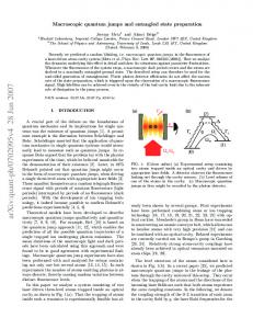
directly the stationary equations using central finite differences and solve the resulting nonlinear system with a damped Newton method. More precisely, we choose the interval (0, 1) and the boundary conditions n(0) = C(0), n(1) = C(1), nx (0) = nx (1) = 0, Jx (0) = Jx (1), V (0) = 0, V (1) = U, where U > 0 is the applied voltage. The numerical scheme is applied to the simulation of a one-dimensional resonant tunneling diode. The device consists of highly doped GaAs regions near the contacts and a lightly doped middle region. The middle region contains a quantum well sandwiched between two AlGaAs barriers (see Figure 1). The double barrier heterostructure is placed between two GaAs spacer layer with a doping of 5 · 1015 cm−3 . These spacers are enclosed by two layers with doping 1018 cm−3 . The double barrier height is 0.209 eV. The physical effect of the barriers is a shift in the quasi-Fermi potential level which we model by an additional step function Vext added to the electrostatic potential. 15

−3

GaAs 10 cm

−3

GaAs

1−x

Al xGa As

GaAs

1−x

Al xGa As

GaAs

−3

0

18

18

GaAs 10 cm

0.209

Energy [eV]

5 10 cm

50

55

60

65

70

75

125

Position [nm]

Figure 1: Geometry of the resonant tunneling diode. In Figure 2 current-voltage characteristics for different choices of the temperature are shown. The effective mass is considered here as a fitting parameter in order to see its influence on the behavior of the curves (also see the discussion in section 3.2). The viscosity depends on the effective mass. The characteristics show several features. First, the current density depends non-monotonously on the applied voltage and there are regions with negative differential resistance, i.e., the current density decreases although the applied voltage increases. The numerical results show that the equations are very sensitive to changes of the parameters. A larger viscosity constant gives a “smoother” curve. Furthermore, as already observed in [67], the curves have a sharp gradient just before the region of negative differential resistance. Physically, a sharp gradient just after the local maximum of the current is expected. The reason of this phenomenon is under investigation. 15

8

8

10

6

x 10

−2

Effective Current Density Jeff [Am ]

Effective Current Density J

eff

[Am−2]

9 8 7 6 5 4 3 2

x 10

5

4

3

2

1

1 0 0

0.05

0.1

0.15 0.2 Voltage U [V]

0.25

0.3

0 0

0.05

0.1

0.15 0.2 Voltage U [V]

0.25

0.3

Figure 2: Current-voltage characteristics of a tunneling diode. Left: temperature T = 300K, meff = 0.067m0 , ν0 = 4.89 (solid) and meff = 0.126m0 , ν0 = 2.60 (dashed). Right: temperature T = 77K, meff = 0.067m0 , ν0 = 1.59 (solid), meff = 0.067m0 , ν0 = 4.77 (dash-dotted), meff = 0.126m0 , ν0 = 2.53 (dashed). The viscosity ν0 is in units of 10−5 m2 /s and m0 is the electron mass at rest.

3.2

Quantum drift-diffusion models

The quantum drift-diffusion model has been recently derived by a diffusion limit from the Wigner equation [29]. We review the main ideas of the derivation using the quantum entropy minimization principle of section 2.4. After introducing the diffusion scaling t → t/δ and Q(w) → Q(w)/δ, the Wigner equation can be written as δ 2 ∂t wδ + δ(p · ∇x wδ + Θ[V ]wδ ) = Q(wδ ),

(27)

where p is the crystal momentum. We are interested in the limit δ → 0, provided the initial condition wδ (·, ·, 0) = wI is given and the quantum collision operator is of BGK-type. In order to make this precise, we introduce first the so-called relative quantum entropy for the density matrix ρ = W −1 [w] (see section 2.4) by Z dxdp w(Ln(w) − 1 + H/T ) , Sq (ρ) = Tr[ρ(ln ρ − 1 + Hq /T )] = (2πε)d R2d where H and Hq are the classical and quantum Hamiltonians, respectively, defined in section 2.4, T > 0 is a fixed temperature, and Ln(f ) := W [ln(W −1 [f ])] for suitable functions f is the “quantum logarithm”. We wish to find, for given n(x), the minimizer of ½ ¾ Z ∗ Sq (ρ ) = min Sq (ρ) : W [ρ]dp = n(x) for all x . Rd

16

The solution (if it exists) is given by ρa = W −1 [wa ], where wa = Exp(a(x) − H/T ). The “quantum exponential” Exp is defined, for suitable R functions f , −1 by Exp(f ) := W [exp(W [f ])]. The function a(x) is such that wa (x, p)dp = n(x). For given w(x, p) we introduce the quantum Maxwellian M [w] by M [w] R := Exp(a − H/T ) such that (M [w] − w)dp = 0, and we assume that this integral constraint fixes the function a(x) uniquely. Now we can make precise the BGK-type collision operator: Q(w) = M [w] − w.

(28)

It models the interaction of the particles with a background heat bath of fixed temperature T . In the limit δ → 0 we see from (27) that the formal limit w0 = limδ→0 wδ satisfies Q(w0 )R = 0, hence w0 = M [w0 ] = Exp(a0 − H/T ) for some a0 (x), and n0 (x) = w0 (x, p)dp/(2πε)d . In [29] it has been further proved by a Chapman-Enskog expansion for wδ that n0 satisfies the equations ∂t n0 − divJ0 = 0,

J0 = T n0 ∇a0 − n0 ∇V,

and n0 and a0 are related by ¶ µ Z dp |p|2 . n0 = Exp a0 (x) − 2T (2πε)d There are up to now no existence results for this model which is of quantum drift-diffusion type. However, some analytical results for a discretized version are shown in [40]. We can expand Exp[a0 (x) − |p|2 /2T ] and thus n0 and J0 in terms of the scaled Planck constant ε. Then n0 = n + O(ε4 ), J0 = J + O(ε4 ), a0 = √ √ ln n − (ε2 /6T )∆ n/ n + O(ε4 ), and n, J satisfy the so-called quantum driftdiffusion equations (up to order ε2 ) [29] µ √ ¶ ∆ n ε2 + T ∇n − n∇V, x ∈ Rd , t > 0. (29) ∂t n − divJ = 0, J = − n∇ √ 6 n Another derivation starts from the isothermal quantum hydrodynamic model (19)-(20), where the right-hand side of (20) is replaced by the momentum relaxation-time term −J/τ . Using the diffusive scaling t → t/τ and J → τ J and the relaxation-time limit τ → 0, n and J are formally satisfying the quantum drift-diffusion equations (29). This limit has been made rigorous for smooth solutions close to the steady state in [62]. The existence of solutions to the stationary equations with mixed DirichletNeumann boundary conditions for the electron density, the quantum quasiFermi potential, and the electrostatic potential is shown in [14]. Existence 17

results on the transient equations in one space dimension have been obtained for different choices of boundary conditions in [65, 69]. For numerical results, we refer to [65, 66]. In this context, we mention that the zero-temperature zero-electric field quantum drift-diffusion equation ¶ ¶ µ µ√ nxx = 0, t > 0, n(·, 0) = nI , x ∈ Rd , ∂t n + n √ n x x also appears in the modeling of interface fluctuations of certain spin systems [32] and has recently attracted the interest of several mathematicians since it possesses some remarkable properties. For instance, the solutions are non-negative, there are several Lyapunov functionals, and related logarithmic Sobolev inequalities can be proved [33]. The existence and uniqueness of solutions, their long-time behavior and numerical solution has been studied in [17, 21, 23, 33, 51, 55, 64, 68]. Quantum drift-diffusion models have been first used by electro-engineers for the simulation of strong inversion layers near the oxide of MOS transistors [2, 4]. It has been also employed for the simulation of source-drain tunneling in MOS transistors [85]. In the engineering literature the quantum drift-diffusion equations are called density-gradient models, and there exists a large number of publications on this subject; see, e.g., [3, 5, 8, 84, 89, 91]. Density-gradient models are also able to predict negative differential resistance effects (i.e. non-monotone behavior) in current-voltage characteristics of tunneling diodes [25, 27, 44, 65, 77, 80]. One important parameter is the socalled peak-to-valley ratio, i.e. the ratio between the maximal and the minimal current value in the current-voltage characteristic. It is well known that the model gives unsatisfactory numerical results at room temperature and with physical (but constant) effective electron mass (see, for instance, [34]). Another view point could be to employ the two constants “temperature” and “effective mass” as parameters to fit experimental data. As an example we present in Figure 3 the current-voltage curve of a tunneling diode using the parameters as in [65] with temperature T = 77K and effective mass meff = 0.067m0 , where m0 is the electron mass at rest. The geometry of the diode is similar to Figure 1 (see [65] for details). The equations are discretized by standard finite differences, and the nonlinear discrete system is solved using Newton’s method. For these parameters the currentvoltage curve shows a region with negative differential resistance. The electrons accumulate in the quantum well if the current density is minimal. In Figure 4 the peak-to-valley ratio (PVR) versus temperature (left) and effective mass (right) is displayed. It turns out that the effective mass appears to be an appropriate parameter to fit the PVR, whereas a change of temperature modifies the ratio only weakly. For temperatures larger than about 130K, 18

9

2.5

x 10

25

10

24

10 Electron density n [m−3]

−2

Current Density J [Am ]

2

1.5

1

0.5

0 0

23

10

22

10

21

10

20

10

19

0.05

0.1

0.15 0.2 0.25 Voltage U [V]

0.3

0.35

10

0.4

0

0.2

0.4 0.6 Position x [nm]

0.8

1

Figure 3: Left: current-voltage characteristic of a tunneling diode at T = 77K. Right: electron densities at the current peak (solid) and current valley (dashed).

8

1.18 1.16

7

Peak to Valley Ratio

Peak to Valley Ratio

1.14 1.12 1.1 1.08 1.06

6 5 4 3

1.04 2

1.02 1

80

90

100 110 Temperature [K]

120

130

1

0.8

1

1.2 1.4 Effective mass [kg]

1.6

1.8 −31

x 10

Figure 4: Peak-to-valley ratios in the current-voltage characteristics of a tunneling diode versus temperature (left) and effective electron mass (right).

19

there is no region of negative differential resistance anymore and the PVR is one. We notice that a non-constant effective mass would be much more physical but the modeling and numerical approximation are more involved (see [88, 89]).

3.3

Hybrid models

Only recently, hybrid quantum models have been derived. In this section, we review two approaches: the coupling of the Schr¨odinger system with the classical drift-diffusion equations and with the quantum drift-diffusion model. Also other hybrid models exist. For instance, we mention the coupled kineticquantum model of [13] and the hybrid classical-quantum equations in [12, 16]. Another approach is to use different models in different spatial directions in order to account for quantum transport in special directions [35]. We assume that the one-dimensional semiconductor domain consists of two parts: a ballistic quantum region, in which the mixed-state Schr¨odingerPoisson system with Lent-Kirkner boundary conditions [38, Appendix D] is solved (see [28, 34] for details), and two diffusion regions near the interval boundary, in which the classical or quantum drift-diffusion model is employed. We have to specify the connection conditions at the two interface points. Consider first the case in which the classical drift-diffusion equations are used in the diffusion regions. A natural condition is to assume the continuity of the current density at the interface. The second condition is derived from a diffusion approximation and a boundary-layer analysis of the reflection-transmission conditions at the interface, based on the model of [13]. This yields a relation between the particle density at the two interface points and the current density [28]. We mention that collisions via the Pauli master equation are included in the ballistic region in [11]. Another approach is to replace the classical drift-diffusion model by the quantum drift-diffusion equations in order to have a consistent quantum description in the whole device. Here, the electron and current densities are assumed to be continuous across the interface points. The current density computed from the Schr¨odinger system depends on the statistics (or “alimentation function”) used in the mixed-state formula. We assume that the statistics of the incoming particles equal the O(ε4 ) approximation of the quantum Maxwellian, introduced in section 3.2, which is related to the quantum driftdiffusion model. This yields nonlinear boundary conditions for the macroscopic electron density and current density. In Figure 5 the current-voltage characteristics of a resonant tunneling diode using the two hybrid models and the mixed-state Schr¨odinger-Poisson system in the whole device are shown. The figure is taken from [34]. We refer to this paper for the choice of the parameters and the numerical method. We 20

7

14

x 10

SP QDD−SP DD−SP

Current density [Am−2]

12 10 8 6 4 2 0 0

0.05

0.1

0.15

0.2

0.25

0.3

0.35

0.4

Voltage [V]

Figure 5: Current-voltage characteristics for a resonant tunneling diode using the Schr¨odinger-Poisson (SP), quantum drift-diffusion Schr¨odinger-Poisson (QDD-SP), and drift-diffusion Schr¨odinger-Poisson (DD-SP) models [34]. see that the numerical results are comparable, with a slightly more diffusive coupled quantum drift-diffusion Schr¨odinger-Poisson (QDD-SP) model. Compared to the full Schr¨odinger-Poisson (SP) model, the CPU time needed for the QDD-SP computations is reduced by about 50%. Since it is possible to derive an analytical expression for the connection conditions in the drift-diffusion Schr¨odinger-Poisson (DD-SP) model, the CPU time for this model compared to the SP system is even reduced by a factor of about 8. This shows that accurate and efficient computations are possible with hybrid quantum models.

References [1] G. Al`ı and G. Frosali. On quantum hydrodynamic models for the two-band Kane system. Preprint, 2004. [2] M. Ancona. Diffusion-drift modeling of strong inversion layers. COMPEL 6 (1987), 11-18. [3] M. Ancona. Finite-difference schemes for the density-gradient equations. J. Comp. Electr. 1 (2002), 435-443. [4] M. Ancona and G. Iafrate. Quantum correction to the equation of state of an electron gas in a semiconductor. Phys. Rev. B 39 (1989), 9536-9540. [5] M. Ancona, Z. Yu, W. Lee, R. Dutton, and P. Voorde. Density-gradient simulations of quantum effects in ultra-thin-oxide MOS structures. SISPAD 97 (1997), 97-100.

21

[6] P. Argyres. Quantum kinetic equations for electrons in high electric and phonon field. Phys. Lett. A 171 (1992), 373-379. [7] A. Arnold, J. Lopez, P. Markowich and J. Soler. An analysis of quantum FokkerPlanck models: a Wigner function approach. To appear in Rev. Mat. Iberoam., 2004. [8] A. Asenov, G. Slavcheva, A. Brown, J. Davies, and S. Saini. Increase in the random dopant induced threshold flutuations and lowering in sub-100nm MOSFETs due to quantum effects: a 3-D density-gradient simulation study. IEEE Trans. Electr. Dev. 48 (2001), 722-729. [9] N. Ashcroft and N. Mermin. Solid State Physics. Sanners Collegs, Philadelphia, 1976. [10] J. Barker and D. Ferry. Self-scattering path-variable formulation of high-field, time-dependent, quantum kinetic equations for semiconductor transport in the finite collision-duration regime. Phys. Rev. Lett. 42 (1979), 1779-1781. [11] M. Baro, N. Ben Abdallah, P. Degond, and A. El Ayyadi. A 1D coupled Schr¨odinger drift-diffusion model including collisions. Preprint No. 923, WIAS Berlin, Germany, 2004. [12] M. Baro, H.-C. Kaiser, H. Neidhardt, and J. Rehberg. A quantum transmitting Schr¨odinger-Poisson system. To appear in Rev. Math. Phys., 2004. [13] N. Ben Abdallah. A hybrid kinetic-quantum model for stationary electron transport in a resonant tunneling diode. J. Stat. Phys. 90 (1998), 627-662. [14] N. Ben Abdallah and A. Unterreiter. On the stationary quantum drift-diffusion model. Z. Angew. Math. Phys. 49 (1998), 251-275. [15] P. Bhatnagar, E. Gross, and M. Krook. A model for collision processes in gases. I. Small amplitude processes in charged and neutral one-component systems. Phys. Review 94 (1954), 511-525. [16] B. Biegel. Simulation of ultra-small electronic devices: the classical-quantum transition regime. NASA Technical Report 97-028, 1997. [17] P. Bleher, J. Lebowitz, and E. Speer. Existence and positivity of solutions of a fourth-order nonlinear PDE describing interface fluctuations. Commun. Pure Appl. Math. 47 (1994), 923-942. [18] K. Brennan. The Physics of Semiconductors. World Scientifc, Singapore, 1999. [19] L. Brillouin. La m´echanique ondulatoire de Schr¨odinger: une m´ethode g´en´erale de r´esolution par approximations successives. Comptes Rendus 183 (1926), 2426.

22

[20] F. Bornemann, P. Nettesheim, and C. Sch¨ utte. Quantum-classical molecular dynamics as an approximation to full quantum dynamics. Preprint, KonradZuse-Zentrum Berlin, Germany, 1995. [21] M. C´aceres, J.A. Carrillo, and G. Toscani. Long-time behavior for a nonlinear fourth order parabolic equation. To appear in Trans. Amer. Math. Soc., 2004. [22] A. Caldeira and A. Leggett. Path integral approach to quantum Brownian motion. Phys. A 121A (1983), 587-616. [23] J.A. Carrillo, A. J¨ ungel and S. Tang. Positive entropic schemes for a nonlinear fourth-order equation. Discrete Contin. Dynam. Sys. B 3 (2003), 1-20. [24] F. Castella, L. Erd¨os, F. Frommlet, and P. Markowich. Fokker-Planck equations as scaling limits of reversible quantum systems. J. Stat. Phys. 100 (2000), 543601. [25] P. Caussignac, J. Descloux, and A. Yamnahakki. Simulation of some quantum models for semiconductors. Math. Models Meth. Appl. Sci. 12 (2002), 1049-1074. [26] Z. Chen. A finite element method for the quantum hydrodynamic model for semiconductor devices. Comput. Math. Appl. 31 (1996), 17-26. [27] Z. Chen, B. Cockburn, C. Gardner, and J. Jerome. Quantum hydrodynamic simulation of hysteresis in the resonant tunneling diode. J. Comput. Phys. 117 (1995), 274-280. [28] P. Degond and A. El Ayyadi. A coupled drift-diffusion model for quantum semiconductor device simulations. J. Comp. Phys. 181 (2002), 222-259. [29] P. Degond, F. M´ehats, and C. Ringhofer. Quantum hydrodynamic models derived from the entropy principle. To appear in Contemp. Math., 2004. [30] P. Degond and C. Ringhofer. Binary quantum collision operators conserving mass, momentum and energy. C. R. Acad. Sci. Paris, S´er. I 336 (2003), 785790. [31] P. Degond and C. Ringhofer. Quantum moment hydrodynamics and the entropy principle. J. Stat. Phys. 112 (2003), 587-628. [32] B. Derrida, J. Lebowitz, E. Speer, and H. Spohn. Fluctuations of a stationary nonequilibrium interface. Phys. Rev. Lett. 67 (1991), 165-168. [33] J. Dolbeault, I. Gentil, and A. J¨ ungel. A nonlinear fourth-order parabolic equation and related logarithmic Sobolev inequalities. Preprint, Universit¨at Mainz, Germany, 2004. [34] A. El Ayyadi and A. J¨ ungel. Semiconductor simulations using a coupled quantum drift-diffusion Schr¨odinger-Poisson model. Preprint, Universit¨at Mainz, Germany, 2004.

23

[35] C. de Falco, E. Gatti, A. Lacaita, and R. Sacco. Quantum-corrected driftdiffusion model for transport in semiconductor devices. Preprint, MOX, Politecnico di Milano, Italy, 2004. [36] D. Ferry and H. Grubin. Modelling of quantum transport in semiconductor devices. Solid State Phys. 49 (1995), 283-448. [37] D. Ferry and J.-R. Zhou. Form of the quantum potential for use in hydrodynamic equations for semiconductor device modeling. Phys. Rev. B 48 (1993) 7944-7950. [38] W. Frensley. Boundary conditions for open quantum systems driven far from equilibrium. Rev. Modern Phys. 62 (1990), 745-791. [39] F. Frommlet, P. Markowich, and C. Ringhofer. A Wigner function approach to phonon scattering. VLSI Design 9 (1999), 339-350. [40] S. Gallego and F. M´ehats. Numerical approximation of a quantum driftdiffusion model. C. R. Acad. Sci. Paris, S´er. I 339 (2004), 519-524. [41] I. Gamba and A. J¨ ungel. Positive solutions to singular and third order differential equations for quantum fluids. Arch. Rat. Mech. Anal. 156 (2001), 183-203. [42] I. Gamba and A. J¨ ungel. Asymptotic limits for quantum trajectory models. Commun. Part. Diff. Eqs. 27 (2002), 669-691. [43] I. Gamba and P. Zhang. Work in preparation, 2004. [44] C. Gardner. The quantum hydrodynamic model for semiconductor devices. SIAM J. Appl. Math. 54 (1994), 409-427. [45] C. Gardner and C. Ringhofer. Smooth quantum potential for the hydrodynamic model. Phys. Rev. E 53 (1996), 157-167. [46] C. Gardner and C. Ringhofer. Approximation of thermal equilibrium for quantum gases with discontinuous potentials and application to semiconductor devices. SIAM J. Appl. Math. 58 (1998), 780-805. [47] C. Gardner and C. Ringhofer. The Chapman-Enskog expansion and the quantum hydrodynamic model for semiconductor devices. VLSI Design 10 (2000), 415-435. [48] I. Gasser and P. A. Markowich. Quantum hydrodynamics, Wigner transforms and the classical limit. Asympt. Anal. 14 (1997), 97-116. [49] I. Gasser, P. Markowich, and C. Ringhofer. Closure conditions for classical and quantum moment hierarchies in the small-temperature limit. Transp. Theory Stat. Phys. 25 (1996), 409-423.

24

[50] I. Gasser, P. Markowich, D. Schmidt, and A. Unterreiter. Macroscopic theory of charged quantum fluids. In: P. Marcati et al. (eds.). Mathematical Problems in Semiconductor Physics. Research Notes in Mathematics Series 340 (1995), 42-75, Pitman. [51] U. Gianazza, G. Savar´e, and G. Toscani. A fourth-order nonlinear PDE as gradient flow of the Fisher information in Wasserstein spaces. Preprint, Universit`a di Pavia, Italy, 2004. [52] H. Grubin and J. Kreskovsky. Quantum moment balance equations and resonant tunneling structures. Solid State Electr. 32 (1989), 1071-1075. [53] M. Gualdani and A. J¨ ungel. Analysis of the viscous quantum hydrodynamic equations for semiconductors. To appear in Europ. J. Appl. Math., 2004. [54] M. Gualdani, A. J¨ ungel, and G. Toscani. Exponential decay in time of solutions of the viscous quantum hydrodynamic equations. Appl. Math. Lett. 16 (2003), 1273-1278. [55] M. Gualdani, A. J¨ ungel, and G. Toscani. A nonlinear fourth-order parabolic equation with non-homogeneous boundary conditions. Preprint, Universit¨at Mainz, Germany, 2004. [56] M. T. Gyi and A. J¨ ungel. A quantum regularization of the one-dimensional hydrodynamic model for semiconductors. Adv. Diff. Eqs. 5 (2000), 773-800. [57] F. Huang, H.-L. Li, A. Matsumura, and S. Odanaka. Well-posedness and stability of multi-dimensional quantum hydrodynamics in whole space. Submitted for publication, 2004. [58] A. J¨ ungel. A steady-state quantum Euler-Poisson system for semiconductors. Commun. Math. Phys. 194 (1998), 463-479. [59] A. J¨ ungel. Quasi-hydrodynamic Semiconductor Equations. Birkh¨auser, Basel, 2001. [60] A. J¨ ungel and H.-L. Li. Quantum Euler-Poisson systems: existence of steady states. To appear in Archivum Math., 2004. [61] A. J¨ ungel and H.-L. Li. Quantum Euler-Poisson systems: global existence and exponential decay. To appear in Quart. Appl. Math., 2004. [62] A. J¨ ungel, H.-L. Li, and A. Matsumura. The relaxation-time limit in the quantum hydrodynamic equations for semiconductors. Preprint, Universit¨at Mainz, Germany, 2004. [63] A. J¨ ungel, M. C. Mariani and D. Rial. Local existence of solutions to the transient quantum hydrodynamic equations. Math. Models Meth. Appl. Sci. 12 (2002), 485-495.

25

[64] A. J¨ ungel and R. Pinnau. Global non-negative solutions of a nonlinear fourthoder parabolic equation for quantum systems. SIAM J. Math. Anal. 32 (2000), 760-777. [65] A. J¨ ungel and R. Pinnau. A positivity-preserving numerical scheme for a nonlinear fourth-order parabolic equation. SIAM J. Num. Anal. 39 (2001), 385-406. [66] A. J¨ ungel and R. Pinnau. Convergent semidiscretization of a nonlinear fourth order parabolic system. Math. Model. Num. Anal. 37 (2003), 277-289. [67] A. J¨ ungel and S. Tang. Numerical approximation of the viscous quantum hydrodynamic model for semiconductors. To appear in Appl. Numer. Math., 2004. [68] A. J¨ ungel and G. Toscani. Exponential decay in time of solutions to a nonlinear fourth-order parabolic equation. Z. Angew. Math. Phys. 54 (2003), 377-386. [69] A. J¨ ungel and I. Violet. The quasineutral limit in the quantum drift-diffusion equations. In preparation, 2004. [70] H. Kramers. Wellenmechanik und halbzahlige Quantisierung. Z. Physik 39 (1926), 828-840. [71] C. Levermore. Moment closure hierarchies for kinetic theories. J. Stat. Phys. 83 (1996), 1021-1065. [72] H.-L. Li and P. Marcati. Existence and asymptotic behavior of the multidimensional quantum hydrodynamic model for semiconductors. Commun. Math. Phys. 245 (2004), 215-247. [73] M. Loffredo and L. Morato. Self-consistent hydrodynamical model for HeII near absolute zero in the framework of stochastic mechanics. Phys. Rev. B 35 (1987), 1742-1747. [74] M. Loffredo and L. Morato. On the creation of quantized vortex lines in rotating HeII. Il Nuovo Cimento 108B (1993), 205-215. [75] E. Madelung. Quantentheorie in hydrodynamischer Form. Z. Physik 40 (1927), 322-326. [76] P. Markowich, C. Ringhofer, and C. Schmeiser. Semiconductor Equations. Springer, Vienna, 1990. [77] S. Micheletti, R. Sacco, and P. Simioni. Numerical simulation of resonant tunneling diodes with a quantum drift-diffusion model. In: W. Schilders, E. ten Maten, and S. Houben (eds.). Scientific Computing in Electrical Engineering, Springer (2004), 313-321. [78] V. Morozov and G. R¨opke. Zubarev’s method of a nonequilibrium statistical operator and some challenges in the theory of irreversible processes. Cond. Matter Phys. 1 (1998), 673-686.

26

[79] P. Pietra and C. Pohl. Weak limits of the quantum hydrodynamic model. In: Proceedings of the International Workshop on Quantum Kinetic Theory, Breckenridge, Colorado, USA, Special Issue of VLSI Design 9 (1999), 427-434. [80] R. Pinnau and A. Unterreiter. The stationary current-voltage characteristics of the quantum drift-diffusion model. SIAM J. Num. Anal. 37 (1999), 211-245. [81] C. Pohl. On the numerical treatment of dispersive equations. PhD thesis, Technische Universit¨at Berlin, Germany, 1998. [82] M. Rudan, A. Gnudi, and W. Quade. A generalized approach to the hydrodynamic model for semiconductor equations. In: G. Baccarani (ed.). Process and Device Modeling for Microelectronics. Elsevier, Amsterdam (1993), 109-154. [83] M. Taylor. Pseudodifferential Operators. Princeton University Press, Princeton, 1981. [84] H. Tsuchiya and T. Miyoshi. Quantum transport modeling of ultrasmall semiconductor devices. IEICE Trans. Electr. E82-C (1999), 880-888. [85] J. Watling, A. Brown, and A. Asenov. Can the density gradient approach describe the source-drain tunnelling in decanano double-gate MOSFETs? J. Comp. Electr. 1 (2002), 289-293. [86] W. Wenckebach. Essentials of Semiconductor Physics. John Wiley & Sons, Chichester, 1999. [87] G. Wentzel. Eine Verallgemeinerung der Quantenbedingungen f¨ ur die Zwecke der Wellenmechanik, Z. Physik 38 (1926), 518-529. [88] A. Wettstein. Quantum Effects in MOS Devices. Series in Microelectronics 94, Hartung-Gorre, Konstanz, 2000. [89] A. Wettstein, A. Schenk, and W. Fichtner. Quantum device-simulation with the density-gradient model on unstructured grids. IEEE Trans. Electr. Dev. 48 (2001), 279-284. [90] E. Wigner. On the quantum correction for thermodynamic equilibrium. Phys. Rev. 40 (1932), 749-759. [91] Z. Yu, R. Dutton, and R. Kiehl. Circuit/device modeling at the quantum level. Proceedings of the Sixth International Workshop on Computational Electronics, Osaka, Japan (1998), 222-229. [92] B. Zhang and J. Jerome. On a steady-state quantum hydrodynamic model for semiconductors. Nonlin. Anal. 26 (1996), 845-856. [93] D. Zubarev, V. Morozov, and G. R¨opke. Statistical Mechanics of Nonequilibrium Processes, Vol. 1. Akademie Verlag, Berlin, 1996.

27