Apr 22, 2009 - signed for quick and easy integration into application codes that ... limited and memory use must be completely transparent to the application developer. ...... each case, suggesting near-perfect parallelism in the data transfer.
MADRE: The Memory-Aware Data Redistribution Engine∗ Stephen F. Siegel
Andrew R. Siegel
April 22, 2009
Abstract We report on the development of a new computational framework for efficiently carrying out parallel data redistribution in a limited memory environment. This new library, MADRE (The Memory-Aware Data Redistribution Engine), is an open-source, C/MPI-based toolkit designed for quick and easy integration into application codes that have demanding data migration needs. At the same time, MADRE exposes a lower-level API that greatly facilitates the development and incorporation of new algorithms into the MADRE framework, thus serving as a potential organizing entity for continued research in this area. Finally, we develop, describe, and test in detail several new parallel redistribution algorithms that are incorporated into the MADRE distribution.
1
Introduction
A large class of massively parallel scientific applications are memory-bound. To achieve their scientific aims, considerable care must be taken to reduce their memory footprint via careful programming techniques, e.g. avoiding unnecessary data copies of main data structures, not storing global meta-data on a single processor, and so forth. The need for efficient many-to-many parallel data movement arises in a wide variety of such scientific applications (e.g., [8]). Adaptive algorithms, for example, require extensive load balancing to ensure an optimal distribution of mesh elements across processors (both in terms of equal balance and spatial locality) [2]. Time-dependent domaindecomposed particle codes are another good example, with frequent re-balancing of the main data structures as particles cross processor boundaries [6]. Typically, such load balancing operations consist of two parts: (1) computing the map that specifies the new destination for each block of data and (2) efficiently carrying out the movement of data blocks to their new location without exceeding the memory available to the application on any process. There has been much research into the first problem, resulting, for example, in numerous efficient algorithms for computing space-filling curves [1]. The second problem, though, ∗
Technical Report 2009/335, Department of Computer & Information Sciences, University of Delaware, April 2009. This research was supported by the National Science Foundation under Grants CCF-0733035 and CCF-0540948 and used resources of the Argonne Leadership Computing Facility at Argonne National Laboratory, which is supported by the Office of Science of the U.S. Department of Energy under contract DE-AC02-06CH11357.
1
has received little attention, especially in the critical case where memory resources are severely limited and memory use must be completely transparent to the application developer. One of the few explorations into memory-efficient solutions to the data redistribution problem was undertaken by A. Pinar and B. Hendrickson [7]. They formulated a “phase”-based class of solution algorithms, showed that the problem of finding a minimal-phase solution is NP-hard, and studied a family of algorithms for approximating minimal solutions. There remain a number of open issues, though. For example, one can envision many other solutions to the redistribution problem that are not based on the concept of migration phases. What are the basic properties of these algorithms and how will they perform relative to the phase-based methods? What is the impact of local data copies on overall algorithmic performance? What algorithms perform best for different areas of parameter space, including memory footprint, available scratch space, data block size, etc? Further theoretical work and experimentation is necessary to address these questions. Our approach to addressing these questions includes several related goals: (1) to package the new algorithms in a way that is readily accessible to application-level developers with little interest in the underlying theory and (2) to provide a clear, open source software architecture together with the rudimentary algorithmic components to encourage the contribution of new methods by algorithm developers throughout the community. These requirements underpin the current design philosophy of MADRE (Memory-Aware Data Redistribution Engine) [9], an open source, C/MPIbased toolkit for the solution of the limited-memory data redistribution problem. In this paper we describe the theory behind the multi-tiered MADRE API, focusing first on the fundamental properties of the local data redistribution problem, then extending this work to the parallel case. Two parallel algorithms are presented, their basic properties are studied in detail, and their performance is compared on a range of synthetic problems.
2
Local Redistribution
We begin with a precise analysis and description of the limited-memory redistribution problem on a single process. We do this both for clarity of exposition and, as we show, because efficient global (parallel) redistribution algorithms are based in large part on efficient solutions to the local problem. Providing access to a highly tuned local block solver is thus a key component of MADRE extensibility. An excerpt of the MADRE interface demonstrating these layers is shown in Figure 1. The goal of the local redistribution problem is to minimize the number of data copies required to redistribute the blocks according to a given map. The problem is similar to an in-place redistribution of an array based on a given permutation. The maps we are considering, however, are more general than permutations. This is because, in our context, some blocks may be “free,” i.e., they do not currently contain useful data. A redistribution map may indicate that a data block be moved to a free space, in which case there is no need to first copy the data in the free space to somewhere else. The redistribution map is therefore not necessarily a permutation, but a more general sort of function we call a transmutation. Much of the standard theory on permutations generalizes to transmutations. The basic results on transmutations presented below have been known for some time in the field of symmetric inverse semigroups [4,5], but in Section 2.1 we give our own concise, self-contained presentation of the exact results needed for the local algorithm. The algorithm itself is described and analyzed in Section 2.2. Proofs of all results can be found in Appendix A. 2
MADRE_Object MADRE_create(void* data, char* strategy, int numBlocks, int blockLength, MPI_Datatype datatype, MPI_Comm comm); MADRE layer void MADRE_redistribute(MADRE_Object madre, int length, Parallel int* destRanks, int* destIndices); Redistribution void MADRE_destroy(MADRE_Object madre); long MADRE_getMem(); . . . MADRE_BMAN_Object MADRE_BMAN_create(int maxArrays, int numBlocks, int numProcs); void MADRE_BMAN_setDestination(MADRE_BMAN_Object bman, BMAN layer int index, int rank , int destIndex); Block Manager int MADRE_BMAN_getDestinationRank(MADRE_BMAN_Object bman, int index); void MADRE_BMAN_sort(MADRE_BMAN_Object bman); . . . MADRE_LRED_Object MADRE_LRED_create(int maxArrays, int numBlocks); LRED layer Local void MADRE_LRED_addArray(MADRE_LRED_Object lred , Redistribution void* blocks, int elementSize, int blockSize); void MADRE_LRED_redistribute(MADRE_LRED_Object lred , int* map);
Figure 1: MADRE software layers
2.1
Transmutations
Let X be a finite set. Intuitively, we are interested in injective functions π from X to X which are not necessarily defined at every point. The following definition just makes this notion precise: Definition 2.1. A transmutation of X is an ordered pair π = (S, f ) where S ⊆ X and f is an injective function from S to X . The set of all transmutations of X is denoted Trans(X). If we think of π in the intuitive way as a function on X , then S is just the set of points on which π is defined. Define a product on Trans(X) as follows: given transmutations π = (S, f ) and σ = (T, g), let πσ = (U, h), where U = {x ∈ T | g(x) ∈ S} and h(x) = f (g(x)) for x ∈ U . On the intuitive level, πσ is the functional composition of π and σ , but is only defined at those points where the composition makes sense. The transmutation (X, idX ), where idX is the identity function on X , will be denoted simply 1X . For any π, σ, τ ∈ Trans(X), we have 1. 1X π = π1X (the identity property), and 2. (πσ)τ = π(στ ) (the associativity property). A set M with a binary operation and identity element e satisfying the identity and associativity properties is known as a monoid [3]. An element a of a monoid M is said to be invertible if there exists b ∈ M such that ab = e = ba. The set of invertible elements of M forms a group. For the 3
monoid Trans(X), the set of invertible elements is {(X, f ) | f : X → X is a 1-1 correspondence}. This group is isomorphic to the group of permutations of X . Although not every element of Trans(X) has an inverse, we can define the pseudo-inverse of any element as follows. Given π = (S, f ) ∈ Trans(X), let σ = (f (S), g), where g is defined by g(f (x)) = x for all x ∈ S . This is well-defined since f is injective. Then σπ = (S, idS ) and πσ = (f (S), idf (S) ). We call σ the pseudo-inverse of π . We next define two basic kinds of transmutations, which form the “building blocks” of Trans(X). Definition 2.2. Let n ≥ 1, and let x1 , . . . , xn be n distinct elements of X . Define f : X → X by xi+1 if x = xi for some 1 ≤ i < n f (x) = x1 if x = xn x if x ̸∈ {x1 , . . . , xn }. The transmutation π = (X, f ) is called a cycle, and is denoted (x1 , . . . , xn ). The length of the cycle is n, and is denoted len(π). Note there are many different ways to denote the same cycle, e.g., (x1 , x2 , x3 ) = (x2 , x3 , x1 ). However, the length of a cycle is well-defined. A cycle is said to be trivial if it has length 1. Clearly, a trivial cycle equals 1X . Definition 2.3. Let n ≥ 1, and let x1 , . . . , xn be n distinct elements of X . Let S = X \ {xn }. Define f : S → X by { xi+1 if x = xi for some 1 ≤ i < n f (x) = x if x ̸∈ {x1 , . . . , xn }. The transmutation π = (S, f ) is called a shift and is denoted [x1 , . . . , xn ]. The length of the shift is n, and is denoted len(π). We now turn to the problem of factoring a transmutation. Definition 2.4. Let π = (S, f ) ∈ Trans(X). The support of π is the set
supp(π) ≡ {s ∈ S | f (s) ̸= s} ∪ (X \ S). Hence the support of π consists of the points that are either “moved” by f or where f is not defined. Definition 2.5. Let π, σ ∈ Trans(X). We say π and σ are disjoint if supp(π) ∩ supp(σ) = ∅. The following is an easy exercise in the definitions: Proposition 2.6. If π and σ are disjoint transmutations of X then 1. πσ = σπ , and 2. supp(πσ) = supp(π) ∪ supp(σ). 4
1
procedure localRedistribute is input: n : Integer, p : array 0..n − 1 of Integer, blocks : array 0..n − 1 of Block;
2 3 4 5 6 7 8 9 10 11 12 13 14 15 16 17 18 19 20 21
q : array 0..n − 1 of Integer; /* used to store pseudo-inverse of p */ tmp : Block; /* temporary space to hold one block when redistributing a cycle */ for i ← 0 to n − 1 do q[i] ← −1; for i ← 0 to n − 1 do /* compute pseudo-inverse and check p is injective */ j ← p[i]; if j ≥ 0 then {assert q[j] < 0; q[j] ← i;} for k ← 0 to n − 1 do while k < n ∧ q[k] < 0 do k ← k + 1; if k = n then break; i ← k ; j ← p[i]; while j ≥ 0 ∧ j ̸= k do {i ← j ; j ← p[i];} if j < 0 then /* shift */ j ← i; i ← q[j]; while i ≥ 0 do {copy(blocks[j], blocks[i]); q[j] ← −1; j ← i; i ← q[j];} else /* cycle */ if i ̸= k then /* non-trivial cycle */ copy(tmp, blocks[j]); while i ̸= k do {copy(blocks[j], blocks[i]); q[j] ← −1; j ← i; i ← q[j];} copy(blocks[j], tmp); q[j] ← −1; Figure 2: Local Redistribution Algorithm
Note that the support of a non-trivial cycle (x1 , . . . , xn ) is {x1 , . . . , xn } (n ≥ 2). The support of a shift [x1 , . . . , xn ] is {x1 , . . . , xn } (n ≥ 1). Hence two of these primitive transmutations are disjoint if the two sets of symbols occurring in their representations do not intersect. The following is proved in Appendix A: Theorem 2.7 (Lipscomb, [4,5]). Every transmutation can be expressed as a product of non-trivial disjoint cycles and shifts. This factorization is unique, up to order. Example 2.8. Let X = {1, 2, 3, 4, 5}, S = {1, 2, 3}, f (1) = 2, f (2) = 1, f (3) = 4, and π = (S, f ). Then π = (12)[34][5] is the unique factorization of π as a product of non-trivial disjoint cycles and shifts. Note. The identity transmutation is considered to have the trivial factorization consisting of no cycles or shifts.
2.2
Local algorithm
The local redistribution problem can be formulated as follows. We are given an array of data blocks indexed from 0 to n − 1, and a transmutation π = (S, f ) on the set X = {0, 1, . . . n − 1}. 5
An algorithm solves the redistribution problem if for all i ∈ S , the contents of block f (i) after redistribution equals the contents of block i before redistribution. We assume the algorithm works by issuing a sequence of instructions of the form copy(s, t), which copies the contents of block t to block s, and that additional “scratch” blocks can be allocated. The MADRE local redistribution algorithm is given in Figure 2. The transmutation π is represented as an integer array p of length n. A negative value for p[i] indicates that i is not in S , i.e., that block i is free. The algorithm begins by checking that f is injective and computing the pseudoinverse of π , storing this in array q (lines 4–7). A non-negative value for q[i] indicates that block i is waiting to receive the contents of block q[i]; a negative value indicates that block i should not be updated. As soon as the correct data is copied into block i, q[i] is set to −1, so that at termination all entries of q will be −1. The algorithm proceeds by discovering the factors in the unique decomposition of π guaranteed by Theorem 2.7. The factors are discovered by iterating over the entries of q , looking for the first non-negative value. The index of this entry is k . We must next discover whether k belongs to a cycle or a shift. This is accomplished by repeatedly applying p until either we return to k or we reach a point i for which p[i] < 0; in the first case we have discovered a cycle, in the second a shift. The redistribution for a shift [x1 , . . . , xm ] (m ≥ 1) is handled by copying data from xm−1 to xm , then from xm−2 to xm−1 , and so on, finally copying from x1 to x2 . The number of copies used to execute the shift is m − 1. The redistribution for a non-trivial cycle (x1 , . . . , xm ) (m ≥ 2) is accomplished by first copying xm to a temporary space, then copying xm−1 to xm , and so on, and finally copying the temporary space to x1 . The number of copies is m + 1. The total number of copies performed by the algorithm is ∑ ∑ ncpy(π) ≡ (len(σ) − 1) + (len(τ ) + 1), τ ∈Cyc(π)
σ∈Shift(π)
where Shift(π) is the set of shift factors in the unique decomposition of π , and Cyc(π) is the set of non-trivial cyclic factors. Theorem 2.9. For any π ∈ Trans(X), ncpy(π) is the minimal number of copies that can occur in a redistribution solution for π . We now consider the complexity of the algorithm as a function of the number of blocks n. We assume the size of a block and the time required to execute copy are constant. Theorem 2.10. The functions for worst-case time and memory consumed by the local redistribution algorithm are both O(n).
3
Distributed Algorithms
We now formally describe the full parallel redistribution problem that was introduced in Section 1. The distributed data redistribution problem generalizes the local problem described in Section 2.2. For the distributed problem we assume a distributed-memory parallel program consisting of N processes. Each process maintains in its local memory a contiguous, fixed-sized array of data blocks of arbitrary fixed size. Let mi be the number of blocks maintained by process i (0 ≤ i < 6
N ). A block is specified by its address (i, j), where i is the process rank and j (0 ≤ j < mi ) is the array index. Let A denote the set of all addresses. A distributed redistribution problem is specified by a transmutation π = (B, f ) ∈ Trans(A). As in the local case, a redistribution algorithm solves the problem if for all b ∈ B , the contents of f (b) after redistribution equal the contents of b before redistribution. The distributed problem may be thought of as an “in-place” version of MPI_ALLTOALLV. The algorithms implemented in MADRE are expected to satisfy certain additional requirements. The first is that each should be a complete algorithmic solution to the data redistribution problem, i.e., it should terminate in finite time with the correct result on any redistribution problem, even one with no free blocks on any process. Second, the additional memory required by the algorithm should depend only linearly on the problem size. To be precise, there must be (reasonably small) constants c1 , c2 , and c3 such that the memory required by the algorithm on process i is at most c1 N + c2 mi + c3 l. Algorithms with a quadratic dependence on the problem size will not scale on current high-end machines. In particular, no single process can store the entire global map π ; it is only given the destination addresses for its own blocks. Finally, each algorithm should consume other resources frugally; e.g., the number of outstanding MPI communication requests on a process must stay within reasonably small bounds. The MADRE library includes a module for the management of blocks on a single process. This module maintains the destination addresses for each block and provides a procedure to sort the blocks on a single process by increasing destination rank (with all free spaces at the end). The sorting procedure uses the local redistribution algorithm of Section 2.2. The distributed algorithms depend heavily on these services, in particular because it is often necessary to create contiguous send and receive buffers. Finally, the algorithms discussed here are restricted to a certain subset of MPI functions (referred to as “permissible” in [10]) that guarantees deterministic behavior. As shown in [10], the advantage gained by this is that the final state arrived at in any execution of the program depends only on the inputs to the program (e.g., the map), and not on any choices made by the MPI implementation. This makes the programs much easier to test and debug.
3.1
A Pinar-Hendrickson Parking Algorithm
Our first algorithm is an instance of the family of “parking” algorithms described in [7]. Pseudocode for the algorithm is given in Figure 3. We first describe a more basic algorithm from [7], and then describe the modifications to the basic version which yield the parking algorithm. The basic algorithm proceeds in a series of global phases. Within each phase, each process receives as much data as possible into its free space while sending out as much data as possible to other processes. When this communication completes, the space occupied by the sent data is reclaimed as free, the blocks are re-sorted, and the next phase begins. This continues until all blocks have arrived at their final destinations. The protocol for determining how many blocks a process p will send and receive to/from other processes in a phase proceeds as follows. First, p informs each process q of the number of blocks it has to send to q . These can be thought of as “requests to send” on the part of p. At the same time, p receives similar requests from the processes that wish to send it data. If p does not have sufficient free space to receive all the incoming data, it uses some heuristic to apportion its free space among its sources. In any case, p sends each source a message stating how much of the request will 7
symbol N out[i] in[i] send[i] recv[i] park[i] ∆[i] free 1 2 3 4 5 6 7 8 9 10 11 12 13 14 15 16 17 18 19 20 21 22 23 24
meaning number of processes number of blocks remaining to send to proc i number of blocks remaining to receive from proc i number of blocks to send to i in current phase number of blocks to receive from i in current phase number of parking blocks to send to i in current phase number parking spaces (−) or blocks to park (+) for proc i (root only) number of free spaces on this proc
procedure main is while true do update out∑ ; done ← ( i out[i] = 0 ? 1 : 0); Allreduce(done, 1, INT, LAND); if done then break; computeDirectMoves(); addParking(); executePhase();
25 26 27 28 29 30 31 32 33 34
procedure computeDirectMoves is Alltoall(out, 1, INT, in, 1, INT); r ← free; for i ← 0 to N − 1 do recv[i] ← min{r, in[i]}; r ← r − recv[i]; Alltoall(recv, 1, INT, send, 1, INT); procedure executePhase is sortBlocks(); foreach {i | recv[i] > 0} do post recv for recv[i] blocks from proc i foreach {i | send[i] > 0} do post send of send[i] blocks to proc i ∑ free ← free + i (send[i] − recv[i]); wait for all requests to complete;
35 36
37 38 39 40 41 42 43 44 45 46
procedure addParking is foreach ∑i do park[i] ← 0; d←∑ ( i in[i]) − free; s ← i send[i]; if d < 0 then δ ← d; else if d > s then δ ← d − s; else δ ← 0; Gather(δ, 1, INT, ∆, 1, INT, root); if myRank = root then foreach {i | ∆[i] > 0} do foreach j do t[j] ← num. parking blocks proc i will send to proc j if i ̸= root then Send(t, N, INT, i); else foreach j do park[j] ← t[j]; else if δ > 0 then Recv(park, N, INT, root) foreach i do send[i] ← send[i] + park[i] Alltoall(send, 1, INT, recv, 1, INT);
Figure 3: A Pinar-Hendrickson parking algorithm be granted, i.e., the number of blocks it will receive from that source in the current phase. (Our implementation uses the first-fit heuristic of [7].) At the same time, p receives similar granting messages from its targets. At this point, p knows how many blocks it will send and receive to/from each process. The data is then transferred by initiating nonblocking send and receive operations for the specified quantities. There are situations in which the basic algorithm described above does not terminate. This can happen, for example, if a cyclic dependency occurs among a set of processes with no free space. 8
Moreover, when it does complete it may take many more phases than necessary. For these reasons, Pinar and Hendrickson introduce “parking.” The idea is that if p does not have enough free space to receive all of its incoming data in the next phase it can temporarily “park” data on processes with extra free space. The parked data will be moved to its final destination when space becomes available. A root process is used in each phase to match processes with data to park with those with extra free space. A parking algorithm will always complete, as long as there is at least one free space on at least one process. (Our implementation allocates a single free space if there are no free spaces at all so that the algorithm will complete in all cases.) Parking can also significantly reduce the number of phases, approximating to within a factor of 1.5 a minimal-phase solution, though this does not always reduce the run-time.
3.2
Cyclic Scheduler
The parking algorithm described above exhibits several potential weaknesses. First, the total quantity of data moved is greater than necessary, because parking blocks are moved more than once. Second, the division into phases, with an effective barrier between each phase, may limit the possible overlap of communication with communication. For example, if some processes require very little time to complete their work in a phase, they will block, waiting for other processes to complete the phase, when they could be working on the next phase. Third, the number of phases may blow up as the total number of free spaces decreases, and there is significant overhead required to execute each phase. Like the parking algorithm, the cyclic scheduler algorithm uses a root process to help schedule actions on other processes. However, it differs in several ways. First, all blocks are moved directly to their final destinations. Second, the cyclic algorithm separates the process of schedule creation from the process of schedule execution. The schedule is created in the first stage of the algorithm, which relies heavily on the root. Once that stage completes, each process has the complete sequence of instructions it must follow in order to complete the redistribution. In the schedule execution stage, each process executes these instructions. In this stage, the root plays no special role, there are no effective barriers, and minimal overhead is required. Since the length of a schedule is bounded above by mi , the memory overhead required to store the schedule is within our required limits. In all of our experiments to date, the time required to complete the schedule creation stage has been insignificant compared to the time required for the execution stage. A schedule is a sequence of actions for a process to follow. There are three types of actions. The first has the form “Send q blocks to process p1 in increments of c blocks,” meaning that the process should send a message to p1 containing c blocks, then another message of c blocks, and so on, until a total of q blocks have been sent. (The final message will consist of q %c blocks if c does not divide q .) The other action types are “Receive q blocks from p2 in increments of c” and “Send q blocks to p1 and receive q blocks from p2 in increments of c.” The last form requires that c blocks be sent and c received, and after those operations have completed, another c are sent and received, and so on. The blocks must be sorted once before an action begins, but do not have to be sorted again until the next action is executed. This is an important point which reduces the overhead associated to executing an action. To create the schedule, the root essentially performs a depth-first search of the transmission graph. This is the weighted directed graph in which the nodes are the process ranks, and there is an edge from i to j of weight k > 0 if i has k blocks to send to j . It is not possible to store the 9
symbol degree[i] stack[i] stackSize weight[i] dest[i] free[i] 1 2 3 4 5 6 7 8 9 10 11 12 13
meaning number of remaining edges departing from proc i in transmission graph ith element in DFS stack containing nodes of transmission graph current size of DFS stack weight of current edge departing from proc i destination node for current edge departing from i current number of free spaces on proc i
procedure main is for i ← 0 to N − 1 do while degree[i] > 0 do push(i); while stackSize > 0 do r ← peek(); if degree[r] = 0 then scheduleShift(); else d ← dest[r]; p ← stackPos[d]; if p < 0 then push(d); else scheduleCycle(p);
14 15 16 17 18 19 20 21 22 23
24 25
procedure scheduleCycle(s) is q ← mini≥s {weight[stack[i]]}; c ← min{q, max{1, mini≥s {free[stack[i]]}}}; l ← peek(); while stackSize > s do p1 ← pop(); p2 ← dest[p1 ]; if stackSize > s then p0 ← peek(); else p0 ← l; schedule send-recv on p1 with source p0 , dest p2 , quantity q , and increment c; weight[p1 ] ← weight[p1 ] − q ; if weight[p1 ] = 0 then nextEdge(p1 );
Figure 4: The cyclic scheduler root scheduling algorithm. entire transmission graph on the root in linear memory. Instead, each process p sends the root one outgoing edge, i.e., the rank r of a single process to which p has data to send and the number of blocks p has to send to r. As soon as the root has received an edge from each process, it begins scheduling actions. This involves decrementing edge weights, and sending actions back to the nonroot processes. When the weight of an edge from p reaches 0, the root requests a new edge from p. Hence edges are continually flowing in to the root and actions are continually flowing out, in a pipelined manner, which is how the memory required by the root is bounded by a constant times the number of processes. The main part of the scheduling algorithm on the root is shown in Figure 4. The root uses a stack to perform the search of the graph. The stack holds nodes in the graph, i.e., process ranks. If p0 and p1 are two consecutive elements in the stack then there is an edge from p0 to p1 . The stack grows until either (a) a cycle is reached, i.e., the destination rank of the edge departing from the last node on the stack is already on the stack, or (b) a node is reached with no remaining outgoing edges (i.e., no data to send). In case (a), an action is scheduled on each process in the cycle, while in case (b), an action is scheduled on each process in the stack. The algorithm for case (a) is shown. The functions for sending actions and retrieving edges are not shown; these involve parameters, such as the number of actions/edges to include in a single message, that provide some control over the memory/time trade-off. In case (a), the number of blocks q to be sent and received by each process is the minimum weight of an edge in the cycle. The increment is usually the minimum number of free spaces for 10
5.5
Park (128 procs) Cyclic (128 procs)
100
5 4.5 Cyclic (0 free blocks) Park (5K free blocks) Cyclic (5K free locks)
4
10
3.5 3 2.5 2
4
8
16
32
64
128
256
512
(a) Simple global cycle 10000
1 12000
1024
14000
16000
18000
20000
22000
24000
(b) Effect of decreasing free memory
Park Cyclic
Park Cyclic
1000
1000 100 100
10 10
1
1 2
4
8
16
32
64
128
256
512
1024
(c) All free space on one process
2
4
8
16
32
64
128
256
512
1024
(d) Global transpose, 5,000 free blocks/proc
Figure 5: Time to redistribute data. In all cases, each process maintains 25,000 memory blocks of 16,000 bytes each and the y -axis is the time in seconds to complete a data redistribution. In (a), (c), and (d), the x-axis shows the number N of processes in logarithmic scale. In (b), (c), and (d) the time is logarithmic. a process in the cycle. However, if there is a process with no free space, the increment is set to 1: in this case an extra free space reserved for this situation will be used to receive each incoming increment. When the cycle has been executed the extra space will again be free. This is the essential fact that guarantees the algorithm will always terminate, though it does require the allocation of an additional block on each process. The actions scheduled in case (b) are similar, though the first element in the stack performs only a send and the last performs only a receive. The algorithm is most effective when it finds many long cycles or shifts with large quantities. The idea is that all of the actions comprising a single cycle/shift can execute in parallel and should take approximately the same amount of time. Moreover, as pointed out above, no local redistribution needs to take place during the execution of an action.
4
Experiments
We report here on a few experiments comparing the performance of the different algorithms. The experiments are designed to test the algorithms in situations of very high data movement and very limited memory. All experiments were executed on the 1024-node IBM Blue Gene/L at Argonne National Laboratory. In each experiment, each process maintains an array of 25,000 blocks, and each block consists of 16,000 bytes. Thus 400 MB are consumed by data, which is a significant portion of the 512 MB total RAM available on each node. In the first experiment, each process has no free space, and wishes to send all 25K blocks to the next process in the cyclic ordering i 7→ (i + 1)%N , where N is again the number of processes. The 11
data redistribution was timed for various values of N . The second experiment is similar, except that each process has 5K free spaces and sends 20K blocks. The results of these two experiments are shown in graph (a) of Figure 5. The time for the parking algorithm to complete the first experiment is not shown because it did not terminate after 30 minutes; the reasons for this will be explained below. Otherwise, the times range from 2.5 to 5.5 seconds and remain relatively constant as the number of processes is scaled in each case, suggesting near-perfect parallelism in the data transfer. The third experiment is similar to the two above, except that the number of processes was fixed at 128 and the number of blocks to be transferred was scaled from 12K to 25K. (Equivalently, the number of free spaces was decreased from 13K to 0.) The results are shown in graph (b) of Figure 5, and illustrate how the time of the parking algorithm blows up with the decreasing amount of free space, in contrast with the cyclic algorithm. Our performance analyses reveal that this behavior is not due to the communication patterns, which are essentially the same in both cases. Rather, the difference arises because the parking algorithm requires that data be re-sorted at the end of each phase. In this experiment, the distribution of the blocks on process N − 1 at the end of each phase presents a worst case scenario for the sort: the entire array of blocks must be shifted, requiring on the order of 25K calls to memcpy (of 16 KB) as the free space approaches 0. Moreover, the number of phases approaches 25K as the free space approaches 0, and so the time dedicated to sorting quickly blows up. For the cyclic algorithm, each process need only execute a single sendreceive action of 25K blocks with increment equal to the number of free spaces. Because a sort is only required at the end of each action, the cyclic algorithm performs only one sort for the entire execution. In the fourth experiment, one process has 25K blocks of free space and all others have no free space. Each of the processes with data wishes to send an approximately equal portion of its data to all other processes. The times are shown in Figure 5(c). Both algorithms complete for every process count, though the time clearly grows exponentially for both. In the fifth experiment, each process has 5K free spaces and the map sends block j of process i to position (mi + j)/N of process (mi + j)%N , where m = 20K. (The map is essentially a global transpose of the data matrix.) The results are shown in Figure 5(d). In this case the cyclic algorithm blows up with process count, and cannot scale beyond 128 nodes without exceeding our 30-minute limit. In contrast, the parking algorithm scales reasonably well and completes the 1024-node redistribution in only 28 seconds. Further investigation revealed the reason for the discrepancy. For this redistribution problem, the transmission graph is the complete graph in which all edges have approximately equal weight. Moreover, in our implementation each process orders its outgoing edges by increasing destination rank. The result is that all of the actions scheduled by the root are cycles of length 2. These are scheduled in the “dictionary order”
{0, 1}, {0, 2}, . . . , {0, N − 1}, {1, 2}, {1, 3}, . . . , {1, N − 1}, . . . , {N − 1, N }. The execution of one of these pairs involves the complete exchange of data between the two processes. If all exchanges take approximately the same time, execution will proceed in 2N +3 phases: in phase k , the exchanges for all pairs {i, j}, where i + j = k and i ̸= j , will take place. This means that many processes will block when they could be working. For example, in phase 1 only processes 0 and 1 will exchange data, while all other processes wait. In contrast, the parking algorithm completes in 4 stages for any N . Hence, in this case, the parking algorithm achieves much greater overlap of communication. 12
5
Conclusion
For a certain class of scientific applications, the limited-memory data redistribution problem will become an increasingly important component of overall performance and scalability as we move toward the petascale. Solutions to this problem are difficult and subtle. Solution algorithms can behave in ways that are difficult or impossible to predict using purely analytical means, so experimentation is essential for ascertaining their qualities. We have implemented a practical framework with multiple solutions to the problem, two of which are explored in this paper. A series of simple experiments helped us identify some potential weaknesses in a variant of the Pinar-Hendrickson parking algorithm. We addressed these in a new algorithm, only to discover different situations in which that algorithm also performs poorly. We continue to refine the algorithms presented here and to explore entirely new ones. In addition, we are exploring heuristics capable of predicting which algorithm will perform well on a given problem. It may also be possible to combine different algorithms, so that in certain states the algorithm will be switched dynamically, in the middle of the redistribution. Finally, we are preparing another set of experiments in which we integrate MADRE directly into scientific applications, as opposed to the synthetic experiments reported on here. Acknowledgements. We are grateful to Ali Pinar for answering questions about the parking algorithm and making the code used in [7] available to us. We also thank Anthony Chan for assistance with the Jumpshot performance visualization tool [11].
A
Proofs
Proof of of Theorem 2.7. We first establish some notation. Let S ⊆ X and f : S → X an injective function. For any integer i, we will define a function f i from a subset of X to X . For i = 0, f 0 = idX . For i > 0, f i (x) = f (f i−1 (x)) and the domain of f i consists of all x in the domain of f i−1 such that f i−1 (x) ∈ S . For i < 0, f i (x) is defined if there exists y ∈ X such that f −i (y) = x, in which case f i (x) = y ; this is well-defined since f is injective. Note that f i+j (x) = f i (f j (x)) for any integers i and j and any x for which the expressions are defined. We define
f ∗ (x) = {f i (x) | i ∈ Z and x is in the domain of f i } Note that x ∈ f ∗ (x), by taking i = 0. The proof is by induction on |supp(π)|. If supp(π) = ∅ then π = 1X , which has the trivial factorization. So suppose |supp(π)| ≥ 1 and that the theorem holds for any transmutation with support of size less than |supp(π)|. We will show how to express π as product of disjoint transmutations σ and τ , where τ is a non-trivial cycle or shift and supp(σ) ( supp(π). The inductive hypothesis can then be applied to σ , and Proposition 2.6(2) ensures the factors of σ will all be disjoint from τ , completing the proof. Write π = (S, f ). Let t ∈ supp(π), and T = f ∗ (t). Let σ = (S ∪ T, g), where { x if x ∈ T g(x) = f (x) if x ∈ S \ T . 13
The injectivity of g follows from the injectivity of f and the fact that if x ∈ S \ T then f (x) ̸∈ T . Hence σ ∈ Trans(X) and supp(σ) = supp(π) \ T ( supp(π) as t ∈ T . Let τ = (X \ (T \ S), h), where { x if x ∈ X \ T h(x) = f (x) if x ∈ S ∩ T . The injectivity of h follows from that of f and the fact that if x ∈ S ∩ T then f (x) ∈ T . Hence τ ∈ Trans(X) and supp(τ ) = (T \ S) ∪ (T ∩ supp(π)). Furthermore, it is not possible that τ = 1X . For if this were the case then we would have T \ S = ∅, i.e., T ⊆ S , and hence t ∈ S . The definition of h would then imply f (t) = t, which contradicts that assumption that t ∈ supp(π). It is clear that σ and τ are disjoint and that π = στ . It remains to see that τ is either a cycle or a shift. Case 1: T ⊆ S . We will show τ is a cycle. Since T ⊆ S , f i (t) is defined for every integer i. Since S is finite, there must exist j > k ≥ 0 such that f j (t) = f k (t). Since f is injective, f j−k (t) = t. Let m be the least positive integer such that f m (t) = t. Given any integer i, write i = mq + r, where 0 ≤ r < m. Then f i (t) = f mq+r (t) = f r (f mq (t)) = f r (t). This shows that T = {t, f (t), . . . , f m−1 (t)}, from which it follows τ is the cycle (t, f (t), . . . , f m−1 (t)). Case 2: T ̸⊆ S . We will show τ is a shift. First, it is not possible that f i (t) is defined for all i ≥ 0. For if this were the case, we could argue as in Case 1 to show that f m (t) = t for some m, and from there that T ⊆ S . So let m be the least positive integer such that t is not in the domain of f m . Similarly, it is not possible that f i (t) be defined for all i ≤ 0, so let n be the greatest negative integer such that t is not in the domain of f n . It follows that τ is the shift [f n+1 (t), . . . , f −1 (t), t, f (t), . . . , f m−1 (t)]. Proof of Theorem 2.9. Let µ(π) denote the minimal number of copies that can occur in a solution for π . We first claim that if π = π1 π2 , where π1 and π2 are disjoint transmutations, then µ(π) = µ(π1 ) + µ(π2 ). To see this, note that any copy instruction in a redistribution solution involves copying data that originated in some block. Given any solution for π , the subsequence of copy instructions for data that originated in supp(π1 ) will be a solution for π1 . A similar statement holds for π2 . Since the supports of π1 and π2 are disjoint, µ(π) ≥ µ(π1 ) + µ(π2 ). On the other hand, suppose we are given solutions for π1 and π2 . If the solution for π1 uses any blocks in supp(π2 ), replace these with temporary blocks to get another solution of the same length; likewise for π2 . Now a solution for π can be obtained by appending the solution for π2 to the one for π1 , showing µ(π) ≤ µ(π1 ) + µ(π2 ). This means we only need to show that ncpy(π) = µ(π) for π a cycle or a shift. If π is a shift of length m, there are precisely m − 1 blocks that must be moved to new locations, so clearly µ(π) ≥ m − 1 = ncpy(π), so ncpy(π) = µ(π) in this case. If π is a cycle of length m ≥ 2, there are m blocks that must be moved to new locations. Given any solution, consider the first copy from a block in S ≡ supp(π). The target of this copy cannot be in S , because that would overwrite data that has not yet been copied to another location. Hence the first copy must be into some block not in S . So after this first copy completes, there are still m blocks that need to be copied to their final destinations. Hence µ(π) ≥ m + 1, and we have ncpy(π) = µ(π) in this case as well. Proof of Theorem 2.10. Space is clearly O(n). To see that time is O(n), we argue that the body of each loop is executed no more than n times. This is obvious for the loops on lines 4, 5, and 14
8. The loop on line 9 always begins with a value of k at least one larger than the final value of k from the previous iteration, so can iterate no more than n times. Now, X is the disjoint union of the sets supp(σ) (σ ∈ Cyc(π) ∪ Shift(π)) and the sets {x} (for all x ∈ X such that f (x) = x). After any execution of the body of the loop of line 8, q[x] = −1 for all x in the partition containing k . Since control can only reach line 11 if q[k] ≥ 0, this implies that the inner loops (lines 12, 15, 19) are executed at most once for each σ . Moreover, each inner loop iterates at most once over the elements of supp(σ). Hence the total number of iterations of each inner loop is at most n.
References [1] U. Catalyurek, E. Boman, K. Devine, D. Bozdag, R. Heaphy, and L. Riesen. Hypergraphbased dynamic load balancing for adaptive scientific computations. In Proc. of 21st International Parallel and Distributed Processing Symposium (IPDPS’07). IEEE, 2007.
¨ [2] H. L. deCougny, K. D. Devine, J. E. Flaherty, R. M. Loy, C. Ozturan, and M. S. Shephard. Load balancing for the parallel adaptive solution of partial differential equations. Appl. Numer. Math., 16(1-2):157–182, 1994. [3] J. M. Howie. Fundamentals of Semigroup Theory. Oxford University Press, 1995. [4] S. Lipscomb. Cyclic subsemigroups of symmetric inverse semigroups. Semigroup Forum, 34:243–248, 1986. [5] S. Lipscomb. Symmetric Inverse Semigroups. American Mathematical Society, Providence, RI, 1996. [6] C. Nieter and J. R. Cary. Vorpal: a versatile plasma simulation code. J. Comput. Phys., 196(2):448–473, 2004. [7] A. Pinar and B. Hendrickson. Interprocessor communication with limited memory. IEEE Transactions on Parallel and Distributed Systems, 15(7), July 2004. [8] P. M. Ricker, B. Fryxell, K. Olson, F. X. Timmes, M. Zingale, D. Q. Lamb, P. MacNeice, R. Rosner, and H. Tufo. FLASH: A multidimensional hydrodynamics code for modeling astrophysical thermonuclear flashes. volume 31 of Bulletin of the American Astronomical Society, page 1431, Dec. 1999. [9] S. F. Siegel. The MADRE web page. http://vsl.cis.udel.edu/madre, 2008. [10] S. F. Siegel and G. S. Avrunin. Verification of halting properties for MPI programs using nonblocking operations. In F. Cappello, T. H´erault, and J. Dongarra, editors, Recent Advances in Parallel Virtual Machine and Message Passing Interface, 14th European PVM/MPI User’s Group Meeting, Paris, France, September 30 - October 3, 2007, Proceedings, volume 4757 of Lecture Notes in Computer Science, pages 326–334. Springer, 2007. [11] O. Zaki, E. Lusk, W. Gropp, and D. Swider. Toward scalable performance visualization with Jumpshot. Int. J. High Perform. Comput. Appl., 13(3):277–288, 1999.
15