JOURNAL OF GEOPHYSICAL RESEARCH, VOL. 106, NO. E10, PAGES 23,403–23,417, OCTOBER 25, 2001
Magnetic field of Mars: Summary of results from the aerobraking and mapping orbits M. H. Acun ˜a,1 J. E. P. Connerney,1 P. Wasilewski,1 R. P. Lin,2 D. Mitchell,2 K. A. Anderson,2 C. W. Carlson,2 J. McFadden,2 H. Re`me,3 C. Mazelle,3 D. Vignes,3 S. J. Bauer,4 P. Cloutier,5 and N. F. Ness6 Abstract. The Mars Global Surveyor (MGS) Magnetic Field Investigation was designed to provide fast vector measurements of the ambient magnetic field in the near-Mars environment and over a wide dynamic range. The fundamental objectives of this investigation were to (1) establish the nature of the magnetic field of Mars; (2) develop appropriate models for its representation; and (3) map the Martian crustal remanent field (if one existed) to a resolution consistent with the spacecraft orbit altitude and ground track separation. Important and complementary objectives were the study of the interaction of Mars with the solar wind and of its ionosphere. The instrumentation is a synergistic combination of a twin-triaxial, fluxgate magnetometer system and an electron reflectometer. The twin-magnetometer system allows the real-time detection of spacecraftgenerated fields, while the electron reflectometer adds remote magnetic field sensing capabilities as well as information about the local electron population. After Mars orbit injection in September 1997 and through the aerobraking (AB) and science-phasing orbits (SPO) that followed, observations were acquired from more than 1000 elliptical orbits with periapses ranging from 85 to 170 km above Mars’ surface. Following injection into the final ⬃400 km altitude circular-mapping orbit, data have been acquired from more than 6000 orbits in the fixed 0200 –1400 local time plane. Major results obtained so far by the Magnetometer/Electron Reflectometer (MAG/ER) investigation in the course of the mission include (1) the determination that Mars does not currently possess a magnetic field of internal origin (dynamo), (2) the discovery of linear, strongly magnetized regions in its crust, closely associated with the ancient, cratered terrain of the highlands in the southern hemisphere, and (3) multiple magnetic “cusps” that connect the crustal magnetic sources to the Martian tail and shocked solar wind plasma. The solar wind interaction with Mars is therefore similar in many ways to that at Venus and at an active comet, primarily an ionospheric/atmospheric interaction. A comet-like “magnetic pileup” region and boundary develop that stand off the solar wind, and mass loading by pickup ions of planetary origin plays an important role in defining interaction regions and overall geometry. This paper focuses primarily on the results obtained by the magnetometer (MAG) portion of the investigation during the MGS aerobraking, science-phasing, and mapping orbits. A companion paper on this issue summarizes the results obtained from the Electron Reflectometer (ER) sensor.
1. Investigation Objectives and Primary Science Goals The primary objective of the Mars Global Surveyor (MGS) Magnetic Field Investigation was identical to that of the Mars Observer Magnetic Field Investigation, that is, to establish definitively the nature of the magnetic field of Mars [Albee and 1
NASA Goddard Space Flight Center, Greenbelt, Maryland. Space Sciences Laboratory, University of California, Berkeley, California. 3 Centre d’Etude Spatiale de Rayonnements, Toulouse, France. 4 Institut fu ¨r Meteorologie und Geophysik, Universita¨t Graz, Graz, Austria. 5 Space Science Department, Rice University, Houston, Texas. 6 Bartol Research Institute, University of Delaware, Newark, Delaware. 2
Copyright 2001 by the American Geophysical Union. Paper number 2000JE001404. 0148-0227/01/2000JE001404$09.00
Palluconi, 1990]. An important objective in characterizing the magnetic field was to determine if Mars had a global field of internal origin. Previous spacecraft missions had already established that the planetary magnetic field, if it existed, was weak with an expected surface field strength estimated at ⬍50 nT. The detection of a global magnetic field of internal origin would have implied the existence of dynamo action in the interior of the planet. Dynamo field generation requires the motion of an electrically conducting fluid driven by thermal convection; this information alone provides powerful constraints on the composition, thermal evolution, and dynamics of the interior of the planet. As such, magnetometry is one of very few observational techniques (gravimetry is another) capable of probing the deep interior of a planet from a spacecraft orbiting the planet. The remanent magnetization of SNC meteorites suggested that Mars may have had in its past a surface magnetic field comparable in magnitude to that of the Earth [Curtis and Ness, 1988]. Mars’ thermal evolution is evidenced in the geologic
23,403
˜A ET AL.: MAGNETIC FIELD OF MARS ACUN
23,404
formations and units mapped by the Mariner 9, Viking, and Phobos 2 missions and recently by MGS. Different regions of the Martian crust could have been magnetized with varying strengths and orientations representative of prior epochs of magnetic activity. Therefore an important objective of the MGS magnetometer experiment was to detect and characterize any crustal remanent magnetization although this possibility was considered a challenging task owing to the weakness of the anticipated equatorial surface field (7–17 nT [Axford, 1991]). The original Mars Observer mission called for a direct injection of the spacecraft into a 400 km circular-mapping orbit, and the unambiguous detection of weak crustal fields in the presence of strong, solar wind induced fields would have been a difficult task from this altitude. The special characteristics of the low-periapsis aerobraking orbits used by MGS to reduce spacecraft orbital velocity were immediately recognized as a major advantage for the Magnetometer/Electron Reflectometer (MAG/ER) investigation of crustal fields. They enhanced the magnetometer detection sensitivity by a factor of ⬃50 over that achievable from the mapping orbit and made possible the direct study of the lower Martian ionosphere by the Electron Reflectometer instrument. This orbit geometry, coupled with the unforeseen events associated with engineering anomalies in one of the spacecraft solar panels, combined to yield low-altitude (⬍200 km) magnetic field measurements distributed over ⬃20% of the Martian surface [Acun ˜a et al., 1999]. Mars, like the Earth, is a highly differentiated planet. It is considerably more volatile rich with higher oxidation states available for Fe, implying a greater abundance of FeS, FeO, Fe2O3, and Fe3O4 than the Earth [Pepin and Carr, 1992; Longhi et al., 1992]. We therefore expected a large Fe-FeS core, a FeO-rich mantle, and a thick basaltic crust [Anderson et al., 1977]. The prerequisites for an internal dynamo driven magnetic field (a thermally convecting core) and a superimposed “anomalous” magnetic field due to magnetization of rocks as they cool below the Curie temperature (an iron oxide rich basaltic crust) analogous to the Earth were there. A wide range of questions about the internal constitution and thermal and geologic history of the planet could then be addressed: What is the size and probable composition of the core? What is the character of the main field, and what was it in times past? What is the composition of the Martian crust and upper mantle? What is the internal temperature distribution? What are the internal geometries of the crustal provinces, the volcanic edifices, and perhaps other features such as the canyons and large faults? The MGS results have shed considerable light on these fundamental issues but have also opened up a whole new range of intriguing and unexpected questions about Mars’ early history and thermal evolution. 1.1.
MAG/ER Instrument Description
The Mars Global Surveyor magnetic field experiment is similar to that previously developed for the Mars Observer (MO) mission, which failed to achieve Mars orbit in 1993 [Acun ˜a et al., 1992]. The instrumentation provides fast vector measurements (up to 32 samples/s) of magnetic fields over a very wide dynamic range. The instrument complement includes two redundant triaxial fluxgate magnetometers (MAG) and an electron reflectometer (ER). The vector magnetometers provide in situ sensing of the ambient magnetic field in the vicinity of the MGS spacecraft over the range of ⫾4 nT to ⫾65,536 nT with a digital resolution of 12 bits. The Electron Reflectometer
measures the local electron distribution function in the range of ⬃1 eV to 20 KeV and can be used to infer the strength of the magnetic field remotely, where the electrons are reflected back toward the spacecraft, using directional information provided by the vector magnetometer. This synergistic combination of detectors was designed to increase significantly the sensitivity and spatial resolution achievable from Martian orbit with the vector magnetometer alone [Acun ˜a et al., 1992]. The Mars Global Surveyor spacecraft does not include a boom to separate sensors from the main body (Figure 1) and thus reduce the error introduced in the measurements by spacecraft-generated magnetic fields. Each magnetometer sensor is placed at the outer edge of the articulated solar panels, ⬃5 m from the center of the spacecraft. The electron reflectometer sensor is mounted directly on the spacecraft nadir panel. This “twin-magnetometer” configuration allows the real-time detection of spacecraft-generated fields and provides complete redundancy for the investigation. The MAG/ER configuration was dictated by the reduced size of the MGS spacecraft compared to MO and the limited resources available as spares from the Mars Observer Project. The solar panels were also used for aerobraking of the spacecraft to achieve the final mapping orbit and are articulated about two orthogonal axes with respect to the spacecraft bus (Figure 1). Therefore the orientation of the magnetic field sensors with respect to the spacecraft is variable and follows that of the solar panels, which are controlled to satisfy a variety of engineering requirements. The solar panels were specifically designed to minimize the magnetic fields generated by the circulating currents. However, residual stray fields associated with shunt regulators mounted at the base of the panels and the spacecraft Power Supply Electronics (PSE) assembly were found and have been successfully removed, as described in section 1.5. The magnetometer and electron reflectometer designs have extensive space flight heritage, and similar versions have been flown in numerous missions, the most recent being Lunar Prospector [Lin et al., 1998]. At present, the instruments continue to operate flawlessly, and a minimum of 2–32 vector samples/s of magnetic field data are acquired continuously, depending on the telemetry rate supported. Data acquisition, transmission, and command functions are microprocessor controlled and operating nominally with no known anomalies. The total mass of the MGS MAG/ER instruments is 5.2 kg, and the power consumption is 3.7 W. 1.2.
Data System and Products
The MAG/ER fully redundant Data Processing Unit (DPU) onboard MGS includes the magnetometer analog to digital (A/D) converter and performs all the required operations on the raw data acquired by the fluxgate sensor system and the electron reflectometer. This system formats the source packets to be delivered to the spacecraft data system and monitors experiment status, modes of operation, housekeeping functions, etc. A set of default parameter tables and vectors is associated with the executive software system such that the instrument does not require any commands upon power up for proper initialization and setup. Critical commands are processed by an independent hardware capability without the need for microprocessor intervention or initialization. The Electron Reflectometer sensor is coupled to the magnetometer processor through a serial interface link. Each data packet is 952 bytes long, and separate packets are formatted by the processor for the fluxgate magnetometer and electron reflec-
˜A ET AL.: MAGNETIC FIELD OF MARS ACUN
23,405
Figure 1. Schematic of the Mars Global Surveyor (MGS) spacecraft in mapping phase configuration. The outboard (OB) and inboard (IB) magnetometer sensors are located at the outer edge of the ⫹Y and ⫺Y solar panels. The solar panels and the high-gain antenna (HGA) assembly articulate throughout the mapping phase, orienting the solar panels toward the Sun and the HGA axis toward Earth. Both “rewind” while the spacecraft is shadowed by Mars. The principal spacecraft coordinate axes are defined by the X, Y, Z directions (payload coordinate (PL) system). tometer data. The digitization, data collection, and processing routines are interrupt driven by a real-time signal provided 8 times per second by the spacecraft data system, and hence MAG and ER data are sampled uniformly in time with negligible uncertainty. Data compression techniques are used on the experiment to make maximum use of the assigned bandwidth. The fluxgate magnetometer “raw” data are first averaged and then 6 bit differenced between adjacent averages. These differences are then formatted into the MAG packet. Full 12 bit samples are periodically added to recover the baseline. A particular feature of the differencing technique is that when the differences exceed the 6 bit dynamic range, instead of saturating, the system will transmit the folded-over value (modulo 64 count). This allows the reconstruction of rapidly varying signals that otherwise would be lost. In addition, the onboard software monitors the performance of the 6 bit differencing scheme; if the number of saturated differences exceeds a predetermined value, the DPU will left-shift the differencing scheme by one least significant bit, doubling the dynamic range that can be accommodated. The maximum capability of the system is two left shifts, or, equivalently, an increase of 4 times the differencing dynamic range. This feature has been designed to enhance the detection and measurement of small-scale, highly time variable magnetic field structures such as those associated with the sheath and pileup regions on the dayside. The executive flight
software resides in hard programmed Read Only Memory, but default parameter tables can be modified by ground command. Instrument parameters such as sensor zero offsets and electron reflectometer tables were updated at the time of Mars orbit insertion and are periodically reviewed to maintain calibrations up to date. The general data flow diagram of the Mars Global Surveyor MAG/ER data-processing and analysis system has been given by Acun ˜a et al. [1992]. Engineering diagnostic packets and data packets containing either MAG or ER data are processed as appropriate, and both contain sufficient instrument health and status information for monitoring the performance of the instrumentation. The raw data in the MAG packets are processed to yield a continuous time series of magnetic field vectors at the appropriate temporal resolution corresponding to the spacecraft telemetry mode. ER packets are translated into relevant parameters, energy spectra, reflection coefficients, etc., and time-averaged distribution functions as permitted by the telemetry allocation. The MGS MAG/ER archive data set contains vector magnetic field data acquired by the fluxgate magnetometers, measurements of the electron population by the electron reflectometer instrument, and ancillary data. The data are provided in time series format at a variable time resolution depending on the telemetry rate available to the investigation. Magnetometer and electron reflectometer observations are archived in separate time-ordered ASCII files with identical time tags. The final data set will
23,406
˜A ET AL.: MAGNETIC FIELD OF MARS ACUN
eventually cover the entire mapping, aerobraking, and sciencephasing orbits as well as limited cruise phase observations. Cruise phase observations cannot be completely processed owing to the lack of supplementary engineering data (kernels) early in the mission. All data are currently being reprocessed with a more accurate spacecraft magnetic field model that resulted from analysis of the cruise and January/February 2000 maneuver sequences as described in this paper. The magnetometer data are calibrated and provided in physical units (nT) along with spacecraft ephemeris information and additional useful spacecraft engineering data. The static and dynamic (model) spacecraft magnetic fields are also provided along with the corrected ambient field. The electron reflectometer archive is a time ordered series of electron measurements from the MGS mission. Each record consists of a time tag with 19 scalar data points representing measurements of the electron flux in 19 different energy channels, ranging from 10 eV to 20 keV, with an energy resolution of 25%. Each data point is a measure of the electron flux (cm2 s⫺1 sr⫺1 eV⫺1) averaged over a 360⬚ ⫻ 14⬚ disk-shaped field of view (FOV). During the Mapping Phase, as the spacecraft orbits the planet the ER field of view sweeps out the entire sky (4 steradians) every 58.5 min. This is much longer than the integration time per record (2– 48 s, depending on energy and telemetry rate) and much longer than most timescales of interest in Mars’ plasma environment. Two principal coordinate systems are used to render the data in the MGS MAG/ER archive: Sun-state (SS) and planetocentric (PC). Cartesian representations are used for both coordinate systems. Separate files are used for each coordinate system: the SS files have spacecraft position and ambient magnetic field rendered in the SS coordinate system, and PC files have spacecraft position and ambient field rendered in the PC coordinate system. Additional files have been made available for limited time periods associated with studies of the possible Phobos and Deimos interactions with their environment. These preliminary files contain the same magnetic field data rendered in coordinate systems centered on those bodies. The SS coordinate system is defined using the instantaneous Mars-Sun vector as the primary reference vector (X direction). The X axis lies along this vector and is taken to be positive toward the Sun. The Mars velocity vector (state vector) is the second vector used to define the coordinate system. The negative of the velocity vector is used as a secondary reference vector so that the vector cross product of X and Y yields a vector Z parallel to the northward (upward) normal of the orbit plane of Mars. The SS system is therefore called a Sunstate coordinate system since its principal vectors are the Sun vector and the Mars-state vector. This coordinate system is particularly useful for studies of the solar wind interaction with Mars’ ionosphere. The planetocentric coordinate system is body-fixed and rotates with the body as it spins on its axis. The body rotation axis is the primary vector used to define this coordinate system. Z is taken to lie along the rotation axis and be positive in the direction of angular momentum. The X axis is defined to lie in the equatorial plane of the body, perpendicular to Z, and in the direction of the prime meridian as defined by the International Astronomical Union (IAU). The Y axis completes the right-handed set. This coordinate system is particularly useful for studies of crustal magnetism (and other internal fields, if any). A third system, defined as the spacecraft or payload coordinate system, is used for engineering and spacecraft field
correction purposes only. This system is aligned with the spacecraft principal axes and is shown in Figure 1. Data are archived on CD-ROMs in Level 1 compliance with the International Standardization Organization (ISO) 9660 standard. The data are provided as ASCII tables of time series data. These files are referred to as standard time series files (STS files), and all such files have a STS suffix. Each file has an attached header (called an ODL header, which represents the MAG/ER team’s object definition language, distinct from the Planetary Data System Object Description Language). The attached header contains text documenting the data processing and describing the record structure. 1.3.
Spacecraft-Generated Magnetic Fields
The MGS spacecraft was designed with minimal system constraints concerning magnetic cleanliness with one important exception: the solar array panels where the MAG sensors were mounted. The wiring layout of these assemblies was analyzed and simulated using piecewise linear techniques in order to arrive at an optimum design that would minimize the magnetic field generated at the sensor location under all operational conditions. The in-flight performance of the solar arrays was extremely close to that predicted from the analyses. Other spacecraft subsystems did not perform as well, in particular the Power Supply Electronics (PSE), which even after prelaunch compensation produced a few nanoteslas of dynamic interference. Of particular importance for mapping orbit magnetic contamination were the traveling wave tube amplifiers (TWTA) located behind the high-gain antenna (HGA). The construction of these units includes long linear arrays of strong permanent magnets. During the cruise, aerobraking (AB), and science-phasing orbit (SPO1 and SPO2) phases of the mission the HGA was kept stationary and folded against the spacecraft body. Likewise, the magnetometer sensors mounted on the solar arrays remained largely confined to fixed positions (cruise configuration or array normal spin (ANS)). During these periods the spacecraft field is well represented as a constant bias that was subtracted from the data. However, after injection into the circular-mapping orbit the HGA was deployed, and its articulation mechanism was activated. In the mapping phase the HGA and the solar panels are articulated throughout the orbit, creating a variable spacecraft field background related to the motion of the spacecraft in orbit about Mars. The correction techniques used to quantify and remove the fields associated with the TWTA magnets and the PSE currents are described below. Stray magnetic fields associated with the illumination of the solar panels and resulting currents were minimized by the implementation of compensation wiring loops and mirrorimage cancellation techniques. Owing to aerobraking temperature rise considerations, the MGS solar panel interconnection wiring was placed on only one side of the panel, the same as that of the solar cells. This configuration simplified magnetic compensation by reducing a three-dimensional problem to a one-dimensional problem. The final compensated panels generated ⬍0.4 nT at the location of the sensors under full Sun illumination conditions at Mars except under conditions of grazing angle illumination, where local shadowing disturbed the compensation scheme. Testing of the panels was conducted by forcing currents backward through the solar cell strings to simulate uniform illumination. The success of this effort can be measured by noting that the magnetic field generated by the solar array at the magnetometer sensor location exceeded 500
˜A ET AL.: MAGNETIC FIELD OF MARS ACUN
nT prior to the implementation of the compensation scheme. The solar panel actuators did not produce any detectable perturbation in the measurements. However, solar panel current shunts mounted on the solar array yoke appear to have produced a net interference moment equivalent to a few tenths of a nanotesla at the MAG sensors. 1.4.
Instrument In-Flight Calibration
Spacecraft attitude maneuvers can be used as a powerful calibration tool for magnetic field experiments. The MGS spacecraft was put in a “rotisserie mode” during cruise phase that slowly rotated the spacecraft and magnetic field sensors about the X axis every ⬃120 min. This configuration was maintained for the most part during cruise, aerobraking, and science-phasing orbits and allowed a reasonable estimation of spacecraft fields and zero offsets while the HGA was undeployed. During cruise the solar panels were exercised through a range of angles to attempt to characterize the spacecraft field. These maneuvers were only partially successful. Analysis of the data acquired during the maneuvers revealed another spacecraft field source related to the power subsystem. Since the field produced by this source covaried with the spatial position of the sensors (solar panels), it was not possible to unambiguously separate the effects due to the HGA and PSE. During January and February of 2000, additional articulations of the solar panels and the (now) deployed HGA were carried out to more fully characterize the most significant sources of spacecraft magnetic interference. A special sequence of HGA articulations was performed when the spacecraft was in Mars’ shadow (zero solar array current) so an accurate HGA magnetic field model could be developed. The data acquired during these calibration maneuvers allowed the development of a reasonably accurate magnetic field model for the MGS spacecraft. This effort was completed during the summer of 2000, and the model is currently incorporated in all ongoing and retrospective data-processing activities. 1.5.
Spacecraft Field Estimation and Compensation
The spacecraft field estimation and compensation techniques must account for complex contributions from a variety of sources. The magnetometers measure the superposition of the ambient field plus that produced by different sources on the spacecraft. The spacecraft may generate magnetic fields in many ways, and the estimation problem is largely one of identifying correctly what mechanism or subsystem is responsible for the interference. It is very helpful to conduct specialized prelaunch magnetic tests to identify the most important sources. Often one finds that it is impractical to operate the spacecraft in precisely the manner it will be in space (e.g., powered by solar panels, power subsystem state, component articulations, thermal environment, and so on). Prelaunch screening tests of the MGS spacecraft identified the presence of strong permanent magnet assemblies in the traveling wave tube amplifiers attached to the back of the high-gain antenna. Additional sources associated with the power subsystem wiring were also found and partially compensated, but significant residual fields remained. For the purpose of our analysis, we categorize spacecraft sources as static or dynamic. Static fields are due to permanent magnetization, for example, magnets or magnetized objects. Magnetic fields are also produced by currents, for example, in the power subsystem, solar arrays, batteries, and so on; these often scale with a known current, are time-variable, and are
23,407
called dynamic fields. Other dynamic fields may be created by the motion or articulation of mechanical devices or actuators that incorporate permanent magnets. For MGS, during mapping operations, the HGA is articulated in the frame of reference of the spacecraft (payload coordinates or PL for short) as are the two solar panels upon which the magnetometer sensors are located. Each sensor has an associated zero offset vector (for each dynamic range) that must also be estimated. Note that a spacecraft-generated static magnetic field that is in the same reference coordinates as the sensor (sensor coordinates) will behave as a sensor offset. Since the HGA is constantly articulating, the “static” field of the TWTAs is time-variable as seen by the sensors. The January/February maneuvers were designed to map the magnetic field of the HGA. The solar panels (and MAG sensors) were set at one of several fixed orientations and positions with respect to the main body of the spacecraft, and the HGA was rotated in elevation several times at each position. The field of the HGA could then be determined from the difference between the vector field measured at the two locations of the magnetometer sensors. The difference readings are used to eliminate the time-variable, and mostly much larger, ambient field. A more complete model of the field at each sensor takes into account the possibility of a static field associated with the spacecraft and fixed in PL coordinates (Bc), as well as dynamic fields both fixed in sensor coordinates (Bod) and fixed in payload coordinates (Bcd). The former might arise from imperfect cancellation of the contributions of current loops on the solar panels, and the latter might arise from loops associated with power distribution circuits fixed to the spacecraft body. These sources were to be characterized in cruise and on orbit around Mars. The ambient magnetic field due to Mars in the mapping orbit is large (to 220 nT) and variable and behaves as very large amplitude “common mode noise” in the signals produced by the MAG sensors (it is most useful otherwise). Thus only differences between the measurements made simultaneously by both sensors are used to characterize the spacecraftgenerated magnetic field. Because of traditional definitions associated with dual magnetometer systems mounted along a single boom, we identify the sensor mounted on the ⫹Y solar panel as “outboard” (OB) and that mounted on the ⫺Y solar panel as “inboard” (IB). The magnetic field is modeled in PL coordinates (applies to both sensors) as B pl ⫽ 关H兴B s ⫹ 关T兴B 0 ⫹ B a ⫹ B c ⫹ 关T兴B od ⫹ B cd, where Bpl is the field in Cartesian payload coordinates, Bs is the static field of the HGA assembly in Cartesian coordinates defined in the HGA coordinate system, [H] is the transformation matrix from HGA coordinates to payload coordinates, [T] is the transformation matrix from sensor to payload coordinates, B0 is the constant sensor zero offset vector, Ba is the ambient field in payload coordinates, Bc is the spacecraft body static field in payload coordinates, Bod is the dynamic field in sensor coordinates that scales with the power system currents (in Cartesian coordinates), and Bcd is the spacecraft (body) dynamic field in payload coordinates that scales with the power system currents. We assume that Bod and Bcd scale with the spacecraft current as follows: (1) The IB MAG dynamic field scales with the ⫺Y solar array panel current, and (2) the OB MAG dynamic field scales with the ⫹Y solar array panel current. In the case
23,408
˜A ET AL.: MAGNETIC FIELD OF MARS ACUN
Plate 1. Difference (black line) of the vector magnetic field in PL coordinates (top, B x ; middle, B y ; bottom, B z ) measured by the OB and IB magnetometer sensors during one of the HGA articulation sequences. The blue line shows the difference in the modeled field of the HGA at the OB and IB sensor locations.
of Bcd, the spacecraft body field, we assume that it scales with total current output from the (shunted) arrays (defined as [sao_l] in the engineering telemetry). This is the current that goes into the power distribution system on the spacecraft. We use the observation [Bpl (IB) ⫺ Bpl (OB)] to remove the ambient field Ba. Pure sensor rotations will constrain B0, and coupled displacements/rotations (from solar panel movements) or HGA articulations will be used to constrain the
spacecraft field Bs, modeled as an offset dipole about the HGA origin. A generalized inverse procedure [Connerney, 1981] is used to estimate the parameters of the various sources, e.g., the dipole coefficients of the HGA and the offset of the HGA source from the defined center of the HGA coordinate system or scale factors (in nT/A) for the ( x, y, z) components of the dynamic field associated with solar panel currents. The current spacecraft magnetic field model (used in routine
Plate 2. Map of the magnetic field of Mars at MGS mapping altitude of 400 (⫾20) km. The radial component of the magnetic field (in planetocentric coordinates) associated with crustal sources is illustrated using the color scale shown. Observations used for this map were obtained while the spacecraft was in the shadow of Mars during mapping cycles 1–3 and 10 –12. We plot the median value of all observations for each 3⬚ latitude by 3⬚ longitude bin.
˜A ET AL.: MAGNETIC FIELD OF MARS ACUN 23,409
Plate 3. Orthographic projection of the (radial) magnetic field of Mars at MGS mapping altitude viewed from 30⬚S latitude and 180⬚E longitude. A corresponding albedo image of Mars is shown for reference.
23,410 ˜A ET AL.: MAGNETIC FIELD OF MARS ACUN
˜A ET AL.: MAGNETIC FIELD OF MARS ACUN
data processing) is described in the file 具sc_mod.ker典, included in the current data release. It uses an offset dipole for the HGA field (tests demonstrated that no improvement in the fit resulted from using higher-degree and -order spherical harmonic models), referenced to the HGA coordinate system (which is defined at the end of the HGA boom; see SPICE associated documentation). We found that no additional static spacecraft field contributions were needed, and they are assumed to be nonexistent in the current data release. The dynamic fields produced when the solar panels are illuminated are at present estimated with limited but adequate accuracy and amount to ⬍0.2 nT/A in each sensor. Plate 1 shows an example of one HGA mapping sequence and model fit. The three components of the difference field [Bpl (IB) ⫺ Bpl (OB)] acquired on January 20 –21, 2000, are plotted as a function of time (top, ⌬B x ; middle, ⌬B y ; bottom, ⌬B z ) and compared with the HGA model difference field (blue line). The modeling interval begins shortly after the spacecraft entered Mars’ shadow, at which time the HGA was articulated through its maximum elevation range, and ends minutes before the spacecraft emerges into sunlight. The RMS error of the observed difference (⌬B) compared with the model is 0.5 nT. Note that this figure is the sum of the errors for both magnetometers since we use differences in modeling the spacecraft field. The error is larger when the MGS solar panels are illuminated. Figure 2 shows the HGA model field for each sensor during the same time interval as Plate 1. Observations obtained in the shadow of Mars and corrected for spacecraft fields are estimated to be accurate to 0.5 nT or better. Observations obtained during periods when the solar panels are illuminated are estimated to be accurate to ⬃1 nT. It must be noted that the spacecraft fields illustrated in Plate 1 and Figure 2 are of the order of ⫾4 nT and are substantially less than the perturbations due to the solar wind–ionosphere interaction. 1.6.
Magnetometer Zero Levels
The basic zero level stability of the fluxgate sensors used in the MGS instrumentation has been demonstrated over many space missions such as Voyager 1 and 2 and is of the order of 0.2 nT/yr [Acun ˜a, 1974; Behannon et al., 1977; Acun ˜a et al., 1992]. Hence, for the MGS application the magnetometers’ effective “zero” levels are dominated by spacecraft-generated magnetic fields, which have been modeled and removed as described above. 1.7.
Sensor Alignment and Stability
The intrinsic orthogonality of the MAG sensors was calibrated at the Goddard Space Flight Center Magnetic Test facility and is known to an accuracy of better than 0.02⬚. The angular alignment of the MAG sensors with respect to the payload reference coordinate system (PL) was determined optically and mechanically prior to launch. From the flight data it is estimated that the error in knowledge of the alignment between the two triaxial MAG sensors is ⬍0.5⬚ when the solar panels are aligned parallel to each other. The alignment knowledge for each MAG sensor with respect to the spacecraft reference coordinate system is estimated to be better than 1.0⬚ when all contributions are taken into account. These values have remained stable with time over the course of the mission, and the derived alignment correction matrices are used in the MAG- and SPICE-kernel-based data-processing algorithms.
23,411
Figure 2. Model vector magnetic field in payload coordinates (top, B x ; middle, B y ; bottom, B z ) at the OB (primary) and IB (secondary) magnetometer sensor locations during the HGA articulation sequences shown in Plate 1. The difference of the two appears in Plate 1.
1.8.
Solar Panel Anomaly
Shortly after initiating the first aerobraking maneuvers in 1997, significant spacecraft dynamic perturbations were detected during the periapsis passes and attributed to a known “unlatched” and incomplete deployment condition for the ⫺Y solar panel. Further analysis of all available data suggested possible physical damage to this panel, and the decision was made by the MGS Project to reduce the maximum dynamic pressure allowable for aerobraking. The result of this decision was that MGS remained in the cruise configuration (array normal spin, or ANS) and in a low-periapsis, elliptical orbit for ⬃1 additional year instead of just ⬃2 months. This led to extended observations of the Martian ionosphere and an opportunity to map crustal magnetic sources much closer to the planet than originally intended. From the engineering point of view the MAG sensors, located at the outer edge of the solar panels, acted as sensitive attitude perturbation detectors near periapsis when the ambient magnetic field was strongest. It is interesting that detailed analyses of the MAG data, including differences between the two sensors, confirmed the unlatched condition of the solar
˜A ET AL.: MAGNETIC FIELD OF MARS ACUN
23,412
panel but could not support the conclusion of a damaged panel suggested by other analyses. Later on, during aerobraking the panel in question latched in the fully deployed position and the problem was resolved. 1.9.
Telemetry and Dynamic Performance
The MAG/ER instrumentation includes a significant degree of autonomy that reduces to negligible levels the amount of commanding required for routine operations. The onboard processor receives information from the spacecraft data system regarding the supported downlink data rate and status and adjusts the sampling rates and data formatting accordingly. As discussed above, the raw data acquisition rates are derived from hardware signals that exhibit negligible random jitter or random interrupt latency. This feature of the experiment allows the acquisition of high-quality, high sample rate data sets (up to 32 samples/s of magnetic field data) without artificially coloring the magnetic field power spectrum with spurious signals. A significant number of the existing low-altitude, highresolution data sets were acquired during the science-phasing orbits (SPO1 and SPO2) when the orbit periapsis location precessed slowly over the north polar region [Acun ˜a et al., 1999; D. Brain et al., manuscript in preparation, 2001]. Additional high-resolution data have been acquired in the circularmapping orbit at 400 km when the downlink rates have permitted it.
2. 2.1.
Summary of Science Results Global Magnetic Field
Mars Global Surveyor is the first spacecraft to have obtained magnetic field observations below the Martian ionosphere (⬃170 –200 km). Observations acquired from many periapsis passes over the northern hemisphere and at different longitudes indicated only the existence of weak fields (ⱕ5 nT) below the ionosphere, over regions located remote from the crustal magnetic sources discovered by MGS. This led to an upper limit of ⬃2 ⫻ 1018 A/m2 for the magnitude of a present-day Mars dipole [Acun ˜a et al., 1999]. We have reduced our estimate of the maximum present-day Mars dipole by an order of magnitude, to ⬃2 ⫻ 1017 A/m2 (or 2 ⫻ 1020 G/cm3), by a preliminary analysis of a subset of the mapping data acquired during magnetically “quiet” days. The data set consisted of averages (over 1⬚ in latitude) of the vector field acquired over the night hemisphere, when the solar panels are not illuminated. All averages for which the magnitude of B exceeded 5 nT were rejected, leaving 4842 averages well distributed in longitude but (by a 7:1 ratio) predominately northward of the equator. These data were fit to a centered dipole model, allowing for a uniform external field. The best fitting dipole, with magnitude ⬃2 ⫻ 1017 A/m2, did not fit the observations significantly better than no dipole (RMS residual of 1.89 nT versus 1.93 nT). A dipole of this magnitude produces a field of 0.5 nT at the equator, which may be considered an upper limit for the equatorial field of a putative Mars dipole. The magnetic moment of individual crustal sources is difficult to estimate since the distance to the source and its exact geometry are not well known. Using data acquired at the 400 km mapping altitude, Acun ˜a et al. [1999] estimated the net magnetic moment of the Terra Sirenum region to be of the order of 1.3 ⫻ 1017 A/m2, a value comparable to the new upper limit derived in this paper for the global magnetic moment. Candidate minerals possibly responsible for the observed intense magnetization of
the crustal sources have been discussed by Kletetschka et al. [2000]. We note that an equatorial field of 0.5 nT is not significantly greater than the estimated accuracy of the observation, corrected for spacecraft fields, over the nightside of Mars (dark solar panels). The sampling bias in weak field observations introduced by the abundant crustal magnetization south of the dichotomy boundary could lead to an apparent dipole moment comparable to our upper limit. Furthermore, any residual spacecraft-generated field (beyond that modeled and removed in our data processing) with a systematic variation as the spacecraft moves from pole to pole could lead to an apparent dipole moment comparable to our estimated upper limit. Since the solar panels and the HGA track the Sun and Earth over the dayside and (often) rewind over the nightside, it is not unlikely that any residual spacecraft fields would exhibit a systematic variation as the spacecraft moves in its orbit. Therefore it will be difficult to further reduce the presently derived upper limit of ⬃2 ⫻ 1017 A/m2 for the Mars dipole (0.5 nT equatorial field). These more detailed analyses therefore provide additional support to the initial conclusion that the immediate environment of Mars and its interaction with the solar wind is not significantly influenced by a global-scale, planetary magnetic field [Acun ˜a et al., 1998, 1999]. The discovery by MGS of strong, localized crustal magnetic sources is strong evidence that Mars had a global field of interior origin in the past, raising the fundamental question of when and why its dynamo stopped working. The dynamo and the generation of a magnetic field in the interior of a planet are believed to be the consequence of convection in a fluid metallic core driven by thermal energy. This source of this energy is either gravitational (core-mantle differentiation) or the solidification of the inner core (latent heat). A totally liquid core with minimal convection cannot sustain large-scale dynamo action, and the same extreme condition applies to a totally frozen out core. As discussed by Acun ˜a et al. [1999], the observations acquired during AB2 over the Hellas, Argyre, and other impact basins show no evidence of significant fields, suggesting that the dynamo had ceased to operate or its strength had decreased significantly when these basins were formed, presumably by giant impacts dating to the earliest stages of Mars evolution. It is estimated [Hartmann, 1978, 1995; Neukum and Wise, 1976; Neukum and Hiller, 1981] that the Hellas and Argyre impacts took place ⬍300 Myr after Mars accretion was completed (and hence core formation), therefore suggesting that Mars dynamo cessation predates this epoch. If this hypothesis is correct, Mars has had to lose heat much more rapidly than previously estimated from interior models [Schubert and Spohn, 1990; Schubert et al., 1992; Sohl and Spohn, 1997; Spohn et al., 1998] that predict dynamo activity for at least 1000 Myr under varying assumptions for core composition and heat flux. 2.2. Solar Wind Interaction and the Magnetic Pileup Boundary Our knowledge of the nature of the interaction of Mars with the solar wind was incomplete until the arrival of MGS and the acquisition of close-in magnetic field data. The upper limit on any intrinsic magnetic moment discussed above implies that the interaction of the solar wind with Mars is dominated by the planet’s ionosphere and atmosphere [Acun ˜a et al., 1998]. In addition, between the bow shock and the ionopause, the MGS observations confirmed the existence of a third plasma bound-
˜A ET AL.: MAGNETIC FIELD OF MARS ACUN
ary: the magnetic pileup boundary (MPB). The solar wind interaction with Mars displays both Venus-like [Cloutier et al., 1999] and comet-like [Mazelle et al., 1995] features. The solar wind plasma and frozen-in interplanetary magnetic field (IMF) drape around the obstacle formed by the dayside ionosphere. The magnetic field piles up in front of the obstacle, forming a “magnetic barrier,” the MPB. This boundary is similar to those detected at comets Halley and Grigg-Skjellerup by the Giotto experiments [Mazelle et al., 1989, 1995; Re`me et al., 1993]. Turbulent magnetic fields and energized electrons are observed throughout the magnetosheath region between the shock and the MPB [Acun ˜a et al., 1998]. Similar magnetic field signatures were detected at Mars by the Phobos 2 instruments, and ion measurements identified a composition boundary inside of which ions of planetary origin (i.e., O⫹) dominate [Riedler et al., 1989; Rosenbauer et al., 1989; Lundin et al., 1989]. In addition to charge exchange, electron impact ionization has also been shown to be an important mechanism for the production of pickup ions in this region and their subsequent loss to the solar wind [Crider et al., 2000]. 2.3.
Crustal Magnetic Field
The most significant and surprising result of the MAG/ER investigation to date is the discovery of intensely magnetized regions in the Martian crust. Aided by the aerobraking orbit geometry, the MGS MAG/ER experiment recorded unexpectedly large magnetic fields when the spacecraft was beneath the ionosphere and close to the surface of Mars [Acun ˜a et al., 1998, 1999; Connerney et al., 1999]. The sparse longitude and narrow latitude coverage of the planet by the early MGS orbits led to the initial interpretation of these features as being of small spatial extent but strongly magnetized. Contrary to earlier expectations [Hood and Hartdegen, 1997] no crustal magnetization was detected over the giant volcanic edifices of Tharsis or Elysium. Numerous additional magnetic crustal sources were observed during the science-phasing orbits (SPO1 and SPO2) and second aerobraking (AB2) phases of the mission. For coarse mapping purposes, a sufficiently dense sampling of the Mars crust was acquired by the end of AB2, when enough orbits accumulated such that the orbit separation at periapsis was no more than a few degrees in longitude. The latitude of periapsis progressed southward during AB2 and more frequent and intense magnetic sources were detected, particularly in the range of 120⬚W–210⬚W and 30⬚S– 85⬚S, where fields as large as ⬃1600 nT at periapsis (⬃100 km) were observed [Acun ˜a et al., 1999; Connerney et al., 1999]. The observations show that the majority of the crustal magnetic sources lie south of the dichotomy boundary on the ancient, densely cratered terrain of the highlands and extend ⬃60⬚ south of this boundary. It is inferred that the formation of the dichotomy boundary must postdate the cessation of dynamo action because of the clear magnetic differentiation between the terrains on either side of the boundary. The absence of detectable crustal magnetization north of the dichotomy boundary in spite of a widespread record of active volcanism and magmatic flows suggests that dynamo action had ceased at this stage of thermal evolution and crustal differentiation. The southernmost limit of the crustal magnetization region appears to be associated with the destruction or modification of the magnetized crust by the impacts that created the Argyre and Hellas basins. The distribution of magnetization therefore suggests that processes that took place during the late stages or after the cessation of dynamo action only mod-
23,413
ified the ancient, magnetized, thin crust through deep impacts, magmatic flows, tectonics, or reheating above the Curie point. The weaker crustal magnetic sources detected in the northern hemisphere [Acun ˜a et al., 1999] represent a challenge to this interpretation since the lowland terrain where they are located is significantly younger than the ancient highlands south of the dichotomy boundary where the strong crustal sources are found. Dipole models derived for the north polar sources [Acun ˜a et al., 1998; Ness et al., 1999; L. L. Hood et al., personal communication, 2000] tend to yield source depths approaching 100 km, in rough agreement with the estimated depth to the Curie isotherm in this region [Smith et al., this issue; Zuber et al., 2000]. These magnetic signatures are more likely owing to spatially distributed sources at shallower depth. Complementing the discovery of crustal magnetism at Mars, the MGS MAG/ER experiment observed linear patterns in the intense magnetization of the southern hemisphere, particularly over Terra Sirenum and Terra Cimmeria [Connerney et al., 1999]. These linear magnetic structures, or “magnetic lineations,” suggest that tectonic processes similar to those associated with seafloor spreading at Earth operated at Mars. If this association is correct, it would imply the existence of plate tectonics and magnetic field reversals in Mars’ early history. An early era of plate tectonics, with an enhanced surface heat flux, favors generation of a Mars magnetic field; the chronologies of both are intimately linked [Nimmo and Stevenson, 2000]. However, alternative explanations involving the fracturing of a magnetized, thin crustal layer by tectonic stresses associated with the Tharsis rise must also be considered (Herna´ndezBarosio, personal communication, 2000). 2.4.
Crustal Field From Mapping Orbit
At the 400 km orbit altitude the magnetic fields generated by the interaction of Mars’ atmosphere with the solar wind can at times be appreciable. In mapping crustal magnetization, we seek to minimize the influence of external sources. Following our earlier practice [Acun ˜a et al., 1999], we concentrate on the radial magnetic field component, as this is least influenced by the solar wind interaction. To a very good first approximation, external fields draped over a conducting obstacle will align with the conducting surface (perpendicular to the radial component). Second, in the MGS mapping orbit we obtain oversampled coverage of all latitudes and longitudes accessible to the spacecraft at 400 km orbit altitude. We further reduce the influence of external fields by rejecting all observations acquired under sunlit conditions, using only those acquired over the nightside, where the solar wind interaction induced fields are at a minimum. Plate 2 shows a global map of the magnetic field of Mars at a nearly constant 400 (⫾20) km mapping altitude. Plate 2 shows the radial magnetic field magnitude and sign, with blue and red corresponding to the largest negative and large positive radial fields, as defined by the color bar. The large dynamic range of the field measured at mapping altitude due to crustal magnetization motivated the use of a compressed color scale (see color bar). The contour intervals have been chosen to outline some of the weaker sources, with isomagnetic intervals of ⫾100, 50, 25, and 12.5 nT. The radial field due to crustal sources reaches a maximum of 220 nT in the Terra Sirenum region. This is 20 times the field produced by the strongest terrestrial magnetic anomalies observed at comparable altitude by MAGSAT [Langel et al., 1982]. The maps presented in this paper were produced with a
23,414
˜A ET AL.: MAGNETIC FIELD OF MARS ACUN
subset of our mapping phase observations that could be reprocessed with a correction for spacecraft-generated fields by the deadline for submission of this article. In order to provide complete global coverage, while using only observations acquired over the nightside, we used observations obtained during two seasons on Mars. The southern hemisphere was well sampled during the first three mapping cycles (1999 DOY 67 through 1999 DOY 152 with good observations obtained on 64 of the days in this time period). The northern hemisphere was well sampled during the tenth through twelfth mapping cycles (1999 DOY 321 through 2000 DOY 39 with good observations obtained during 84 of the days in this time period). This set of observations was the most recent data available at the time of submission of this article. The maps were produced in the following manner: (1) data volume was reduced by selecting night side observations and averaging along track, decimating to one average for each 1⬚ of latitude; (2) for each latitude/longitude bin, the median value of all measurements within the bin was chosen as a representative field value for that bin. We used bins of 3⬚ latitude by 3⬚ longitude in size, corresponding to approximately 180 km ⫻ 180 km at the equator. The bin size is large enough to include an adequate number of orbit passes (median of 15/bin) and small compared with the spatial resolution that one can achieve from mapping altitude (⬎400 km); that is, the full spatial resolution of the crustal field has not been limited by the averaging and binning performed. We use a median value for each bin rather than an average value because the median is less influenced by the inclusion of one or two very disparate measurements, compared with the mean or average of all measurements. Note that we have performed no filtering or detrending along track, as is often required for analysis of observations from Earth-orbiting spacecraft. Therefore these maps do not limit observation of long-wavelength magnetic sources. In particular, these maps are relatively free of the artifacts that can arise in such situations, e.g., anomalies that appear elongated perpendicular to the orbit tracks.
3.
Discussion
The global distribution of crustal magnetization on Mars is readily apparent in Plate 2. As reported previously [Acun ˜a et al., 1999], the most intense crustal magnetization is found in the southern highlands, particularly the Terra Sirenum and Terra Cimmeria near 180⬚E longitude. Crustal magnetization appears to be associated with and southward of the crustal dichotomy boundary. The relatively young northern lowlands are relatively weakly magnetized, with notable exceptions near 30⬚E longitude. Plate 3 shows an orthographic projection of the radial component of the Martian field as viewed from 30⬚S latitude and 180⬚E longitude. An image of Mars seen from the same angle is also shown for comparison. Plate 4 shows the same field component in an orthographic projection viewed from 30⬚N latitude and 0⬚E longitude. The north polar region was mapped particularly well at lower altitude (170 –200 km) during the SPO mission phase, and a polar projection of these data is given by Acun ˜a et al. [1999]. The north polar region is also extremely interesting for studies of the Mars solar wind interaction; multiple magnetic “cusps” were detected in this region during the SPO phase, and plasmas of different origin are observed. These topics are discussed in detail in the companion paper by Mitchell et al. [this issue], which summarizes Electron Reflectometer results.
Large regions in the southern hemisphere also appear to be free of significant magnetization; as noted previously, these regions are roughly delineated by large and extended areas that reflect the effects of giant and ancient impacts that formed Argyre and Hellas. A notable exception is the relatively weak (⬃12 nT at 400 km) and isolated feature that appears near 30⬚E longitude and 60⬚S latitude, which also appeared in the aerobraking phase map of Acun ˜a et al. [1999]. The east-west trending linear features in the Terra Sirenum and Terra Cimmeria are quite remarkable, bearing in mind the altitude of observation. These features are the high-altitude expression of magnetic lineations observed at lower altitudes during the aerobraking phase (AB2) of the mission and modeled by Connerney et al. [1999]. The mapping orbit (overflight) data near 180⬚ longitude is consistent with the field predicted by the magnetization model presented by Connerney et al. [1999]. However, the higher altitude of observation results in a loss of spatial resolution, so at mapping altitude we sense the average magnetization over large-scale lengths, many hundreds of kilometers. It is unlikely that such large volumes of material could be uniformly magnetized. Indeed, the observations at lower altitude indicated the existence of structures with a characteristic size at the limit of the spatial resolution afforded by the aerobraking altitude (⬃100 km). In general, one cannot expect that the average magnetization over such scales would be representative of the actual magnetization directions present in the crustal material. Indeed, the limiting spatial resolution afforded by the mapping orbit can be deduced by inspection of Plate 2. The relatively isolated circular features of positive sign near 215⬚E longitude, 8⬚S latitude and 255⬚E, 30⬚S are good examples of how a localized source with approximately outward radial magnetization would appear at mapping altitude. Features that evidence elongation in one or more directions are the result of a distribution of crustal magnetization. Isolated, seemingly unipolar features are in a sense more easily interpreted than a collection of features with different signs. A magnetic source produces no net flux on our mapping surface, so, for example, a horizontal dipole produces a pair of positive and negative features in the radial magnetic field separated by distance comparable to the altitude of observation. A dipole oriented radially produces a circular feature of the appropriate sign and the return flux, spread over a much larger area surrounding the central feature, is nearly undetectable (in such maps). A dipole with orientation within 30⬚ or so of the radial direction will thus appear as a unipolar feature. Also evident in Plate 2 are several remarkable features that are spatially extensive and have circular organization. The circular feature of negative polarity at 225⬚E longitude and 45⬚S latitude appears nearly in the center of a partial ring of opposite polarity, much stronger to the west and south. Another such feature appears near 45⬚E and 15⬚N. We have been unable to reliably associate either feature with a crater or similar geologic feature of the appropriate scale in topographic, gravity, or crustal thickness maps [Zuber et al., 2000; Smith et al., this issue].
4.
Summary
The MGS MAG/ER experiment has been in operation almost continuously since its activation early in the cruise phase of the mission until the present. During the aerobraking and science-phasing orbit phases, which lasted more than one year, as well as the first cycle of the mapping phase, this experiment
Plate 4. Projections similar to those shown in Plate 3 but viewed from 30⬚N latitude and 0⬚E longitude.
˜A ET AL.: MAGNETIC FIELD OF MARS ACUN 23,415
23,416
˜A ET AL.: MAGNETIC FIELD OF MARS ACUN
has been able to acquire a remarkable data set. Its analysis led to the discovery of Mars’ crustal magnetization, the mapping of its global distribution, and the modeling of magnetic lineations most likely associated with large-scale Martian tectonic processes that were unsuspected until now. Detailed observations were also made of the solar wind interaction with Mars, including processes such as electron impact ionization of exospheric neutrals and the formation of multiple magnetic cusps and the population of these magnetic structures with electron plasmas of different origins and characteristics. Recently, the MAG/ER investigation has refined its previous estimate of an upper limit to the present-day Martian global dipole moment, showing that it is ⬃10 times lower than previously estimated. An important achievement of the MAG/ER team is the accurate modeling and correction of spacecraft-generated fields, which became possible only after spacecraft calibration maneuvers were completed in January/February 2000. Complete data sets corresponding to the science-phasing orbits phase and the first cycle of mapping data have been delivered to the Planetary Data System for distribution to the science community at large. Additional data sets will be available in the immediate future as they are processed, incorporating the latest algorithms and corrections derived from calibration activities described in this paper. Acknowledgments. We thank the MSOP office at JPL and Lockheed Martin for their assistance with the design and implementation of the spacecraft calibration maneuvers described in this paper. The contributions of Patricia Lawton, Monte Kaelberer, and Ever Guandique of the MAG/ER data-processing and analysis team are, as always, outstanding and are gratefully acknowledged. D. Brain also provided initial visualization and analysis support for mapping orbit data and high time resolution data sets. The research at U.C. Berkeley (S.S.L.) was supported by NASA grant NAG 5 959. The research at U. Delaware (B.R.I.) was supported by NASA grant NAG 5 3538. The research at CESR was supported by a grant from CNES.
References Acun ˜a, M. H., Fluxgate magnetometers for outer planets exploration, IEEE Trans. Magn., 10, 519 –521, 1974. Acun ˜a, M. H., et al., The Mars Observer Magnetic Fields Investigation, J. Geophys. Res., 97, 7799 –7814, 1992. Acun ˜a, M. H., et al., Magnetic field and plasma observations at Mars: Initial results of the Mars Global Surveyor mission, Science, 279(5357), 1676 –1680, 1998. Acun ˜a, M. H., et al., Global distribution of crustal magnetism discovered by the Mars Global Surveyor MAG/ER experiment, Science, 284(5415), 790 –793, 1999. Albee, A. L., and D. F. Palluconi, Mars Observer global mapping mission, Eos Trans. AGU, 71(39), 1099 –1107, 1990. Anderson, D. L., W. F. Miller, G. V. Latham, Y. Nakamura, M. N. Tokosoz, A. M. Dainty, F. K. Duennebier, A. R. Lazarewicz, R. L. Kovach, and T. C. D. Knight, Seismology on Mars, J. Geophys. Res., 82, 4524 – 4546, 1977. Axford, W. I., A commentary on our present understanding of the Martian magnetosphere, Planet. Space Sci., 39(1–2), 167–173, 1991. Behannon, K. W., M. H. Acun ˜a, L. F. Burlaga, R. P. Lepping, N. F. Ness, and F. M. Neubauer, Magnetic field experiment for Voyagers 1 and 2, Space Sci. Rev., 21, 235–257, 1977. Cloutier, P. A., et al., Venus-like interaction of the solar wind with Mars, Geophys. Res. Lett., 26(17), 2685–2688, 1999. Connerney, J. E. P., The magnetic field of Jupiter: A generalized inverse approach, J. Geophys. Res., 86, 7679 –7693, 1981. Connerney, J. E. P., M. H. Acun ˜a, P. Wasilewski, N. F. Ness, H. Re`me, C. Mazelle, D. Vignes, R. P. Lin, D. Mitchell, and P. Cloutier, Magnetic lineations in the ancient crust of Mars, Science, 284(5415), 794 –798, 1999. Crider, D. H., et al., Evidence of electron impact ionization in the
magnetic pileup boundary of Mars, Geophys. Res. Lett., 27(1), 45– 48, 2000. Curtis, S. A., and N. F. Ness, Remanent magnetism at Mars, Geophys. Res. Lett., 15(8), 737–739, 1988. Hartmann, W. K., Martian cratering, 5, Toward an empirical Martian chronology, and its implications, Geophys. Res. Lett., 5(6), 450 – 452, 1978. Hartmann, W. K., Planetary cratering, 1, The question of multiple impactor populations—Lunar evidence, Meteoritics, 30(4), 451– 467, 1995. Hood, L. L., and K. Hartdegen, A crustal magnetization model for the magnetic field of Mars: A preliminary study of the Tharsis region, Geophys. Res. Lett., 24, 727–730, 1997. Kletetschka, G., P. J. Wasilewski, and P. T. Taylor, Mineralogy of the sources for magnetic anomalies on Mars, Meteorit. Planet. Sci., 35(5), 895– 899, 2000. Langel, R., et al., Initial vector magnetic anomaly map from MAGSAT, Geophys. Res. Lett., 9(4), 273–276, 1982. Lin, R. P., D. L. Mitchell, D. W. Curtis, K. A. Anderson, C. W. Carlson, J. McFadden, M. H. Acun ˜a, L. L. Hood, and A. Binder, Lunar surface magnetic fields and their interaction with the solar wind: Results from Lunar Prospector, Science, 281(5382), 1480 – 1484, 1998. Longhi, J., E. Knittle, J. R. Holloway, and H. Wa¨nke, The bulk composition, mineralogy and internal structure of Mars”, in Mars, edited by H. H. Kieffer et al., pp. 184 –208, Univ. of Ariz. Press, Tucson, 1992. Lundin, R., A. Zakharov, R. Pellinen, H. Borg, B. Hultqvist, N. Pisarenko, E. M. Dubinin, S. W. Barabash, I. Liede, and H. Koskinen, First measurements of the ionospheric plasma escape from Mars, Nature, 341, 609 – 612, 1989. Mazelle, C., et al., Analysis of suprathermal electron properties at the magnetic pile-up boundary of comet p-Halley, Geophys. Res. Lett., 16(9), 1035–1038, 1989. Mazelle, C., et al., Comparison of the main magnetic and plasma features in the environments of comets Grigg-Skjellerup and Halley, Adv. Space. Res., 16(4), 41– 45, 1995. Mitchell, D. L., et al., Probing Mars’ crustal magnetic field and ionosphere with the MGS Electron Spectrometer, J. Geophys. Res., this issue. Ness, N. F., et al., MGS magnetic fields and electron reflectometer investigation: Discovery of paleomagnetic fields due to crustal remanence, Adv. Space Res., 23(11), 1879 –1886, 1999. Neukum, G., and K. Hiller, Martian ages, J. Geophys. Res., 86(B4), 3097–3121, 1981. Neukum, G., and D. U. Wise, Mars—Standard crater curve and possible new time scale, Science, 194(4272), 1381–1387, 1976. Nimmo, F., and D. J. Stevenson, Influence of early plate tectonics on the thermal evolution and magnetic field of Mars, J. Geophys. Res., 105, 11,969 –11,979, 2000. Pepin, R. O., and M. H. Carr, Major issues and outstanding questions, in Mars, edited by H. H. Kieffer et al., pp. 120 –146, Univ. of Ariz. Press, Tucson, 1992. Re`me, H., Mazelle C., Sauvaud J. A., et al., Electron-plasma environment at comet Grigg-Skjellerup: General observations and comparison with the environment at comet Halley, J. Geophys. Res., 98(A12), 20,965–20,976, 1993. Riedler, W., et al., Magnetic field near Mars: First results, Nature, 341, 604 – 607, 1989. Rosenbauer, H., et al., Ions of Martian origin and plasma sheet in the Martian magnetosphere: Initial results of the TAUS experiment, Nature, 341, 612– 614, 1989. Schubert, G., and T. Spohn, Thermal history of Mars and the sulfurcontent of its core, J. Geophys. Res., 95(B9), 14,095–14,104, 1990. Schubert, G., S. C. Solomon, D. L. Turcotte, M. J. Drake, and N. H. Sleep, Origin and thermal evolution of Mars, in Mars, edited by H. H. Kieffer et al., pp. 147–183, Univ. of Ariz. Press, Tucson, 1992. Sohl, F., and T. Spohn, The interior structure of Mars: Implications from SNC meteorites, J. Geophys. Res., 102(E1), 1613–1635, 1997. Spohn, T., F. Sohl, and D. Breuer, Mars, Astron. Astrophys. Rev., 8(3), 181–235, 1998. Smith, D. E., et al., Mars Orbiter Laser Altimeter (MOLA): Experiment summary after the first year of global mapping of Mars, J. Geophys. Res., this issue. Zuber, M. T., et al., Internal structure and early thermal evolution of
˜A ET AL.: MAGNETIC FIELD OF MARS ACUN Mars from Mars Global Surveyor topography and gravity, Science, 287, 1788 –1793, 2000. M. H. Acun ˜a, J. E. P. Connerney, and P. Wasilewski, NASA Goddard Space Flight Center, Planetary Magnetospheres Branch, Code 695, Greenbelt, MD 20771. (
[email protected]) K. A. Anderson, C. W. Carlson, R. P. Lin, J. McFadden, and D. Mitchell, Space Sciences Laboratory, University of California, Berkeley, CA 94720. S. J. Bauer, Institut fu ¨r Meteorologie und Geophysik, Universita¨t Graz, Graz, Austria.
23,417
P. Cloutier, Space Science Department, Rice University, Houston, TX 77001. C. Mazelle, H. Re`me, and D. Vignes, Centre d’Etude Spatiale des Rayonnements, Toulouse, France. N. F. Ness, Bartol Research Institute, University of Delaware, Newark, DE 19711.
(Received September 29, 2000; revised February 8, 2001; accepted February 19, 2001.)
23,418