The Astrophysical Journal, 828:83 (15pp), 2016 September 10
doi:10.3847/0004-637X/828/2/83
© 2016. The American Astronomical Society. All rights reserved.
MAGNETO-FRICTIONAL MODELING OF CORONAL NONLINEAR FORCE-FREE FIELDS. II. APPLICATION TO OBSERVATIONS 1
Y. Guo1,2, C. Xia2, and R. Keppens1,2
School of Astronomy and Space Science, Nanjing University, Nanjing 210023, China;
[email protected] 2 Centre for mathematical Plasma-Astrophysics, Department of Mathematics, KU Leuven, B-3001 Leuven, Belgium Received 2016 March 10; revised 2016 May 24; accepted 2016 June 16; published 2016 September 7
ABSTRACT A magneto-frictional module has been implemented and tested in the Message Passing Interface Adaptive Mesh Refinement Versatile Advection Code (MPI-AMRVAC) in the first paper of this series. Here, we apply the magneto-frictional method to observations to demonstrate its applicability in both Cartesian and spherical coordinates, and in uniform and block-adaptive octree grids. We first reconstruct a nonlinear force-free field (NLFFF) on a uniform grid of 1803 cells in Cartesian coordinates, with boundary conditions provided by the vector magnetic field observed by the Helioseismic and Magnetic Imager (HMI) on board the Solar Dynamics Observatory (SDO) at 06:00 UT on 2010 November 11 in active region NOAA 11123. The reconstructed NLFFF successfully reproduces the sheared and twisted field lines and magnetic null points. Next, we adopt a three-level block-adaptive grid to model the same active region with a higher spatial resolution on the bottom boundary and a coarser treatment of regions higher up. The force-free and divergence-free metrics obtained are comparable to the run with a uniform grid, and the reconstructed field topology is also very similar. Finally, a group of active regions, including NOAA 11401, 11402, 11405, and 11407, observed at 03:00 UT on 2012 January 23 by SDO/HMI is modeled with a five-level block-adaptive grid in spherical coordinates, where we reach a local resolution of 0 . 06 pixel−1 in an area of 790 Mm×604 Mm. Local high spatial resolution and a large field of view in NLFFF modeling can be achieved simultaneously in parallel and block-adaptive magneto-frictional relaxations. Key words: methods: numerical – Sun: corona – Sun: magnetic fields 1. INTRODUCTION
Amari 2010; Cheng et al. 2010; Guo et al. 2010a, 2010b; Jing et al. 2010), magnetic null points (Zhang et al. 2012; Sun et al. 2013, 2014), and quasi-separatrix layers (Savcheva et al. 2012, 2015; Guo et al. 2013; Zhao et al. 2014; Yang et al. 2015). Most of them are modeled in Cartesian coordinates, although some models are reconstructed in spherical geometry (Su et al. 2009; Tadesse et al. 2011; Guo et al. 2012) or with tetrahedral meshes (Amari et al. 2014b). In particular, Amari et al. (2014a) has developed another code to fulfill the need for reconstructions on the scale of local active regions within a global extrapolation, using an iterative Grad– Rubin scheme adapted to spherical coordinates. Such a state-ofthe-art code resolves an active region in a global model with 120 ´ 200 ´ 340 grid points. This contrasts to most earlier modeling efforts, which were limited either to a small field of view (for Cartesian coordinates) or to lower spatial resolution (for spherical coordinates) due to limited computational resources. The data volume and the computation time increase for NLFFF modeling with a large field of view and high spatial resolution simultaneously, which implies a big data problem. On the other hand, we have to use data with high spatial resolution to resolve the small-scale features of the magnetic field, such as small flux tubes and electric current channels. They are crucial for reconstructing the non-potential magnetic field. We also have to consider a field of view as large as possible to include remote magnetic field connections (DeRosa et al. 2009). Since only the bottom boundary is available at present for realistic NLFFF modeling, the magnetic field concentration should be isolated to mitigate any effects of lateral boundary conditions (Wiegelmann et al. 2006). An isolated magnetic field region has magnetic field lines originating from the bottom boundary and connecting back to the bottom. A large field of view is required to fulfill this
The solar atmosphere is filled with magnetized plasma and displays many activities, such as magnetic flux rope eruptions, flares, coronal mass ejections, magnetohydrodynamic (MHD) waves, and so on. All these activities depend crucially on the density, temperature, and velocity of the plasma, and most importantly on the three-dimensional (3D) distribution of the magnetic field. Because of the conditions of high conductivity and low plasma β (the ratio between gas and magnetic pressure) in the solar corona, the magnetic field governs the structure and dynamics of coronal plasma. However, the magnetic field can only be routinely and relatively accurately observed in the photosphere. Extrapolations of the magnetic field from the bottom boundary have existed for a long time (Schmidt 1964). Initially, a potential field without any electric current was adopted due to the limited observational and computational techniques. A potential field model does provide a crude approximation for the large-scale solar magnetic structures, and is appropriate when little electric current is present. Later on, linear force-free field modeling was developed with a constant α, the torsional parameter representing the global proportionality between the electric current and the magnetic field (Nakagawa & Raadu 1972; Chiu & Hilton 1977; Seehafer 1978; Alissandrakis 1981). However, observations show that α is usually not constant for the solar magnetic field (Régnier et al. 2002; Wiegelmann & Neukirch 2002; Schrijver et al. 2005). Therefore, a more realistic force-free field model with non-constant α, the nonlinear force-free field (NLFFF), is required at least to compute the 3D magnetic field in the corona (Wiegelmann & Sakurai 2012 and references therein). NLFFF models have been widely adopted to study magnetic field structures in the solar atmosphere, for instance, magnetic flux ropes (Canou et al. 2009; Su et al. 2009; Canou & 1
The Astrophysical Journal, 828:83 (15pp), 2016 September 10
Guo, Xia, & Keppens
The transverse component of the vector magnetic field bears an intrinsic 180 ambiguity, which is resolved by the use of an improved version of the minimum energy method (Metcalf 1994; Metcalf et al. 2006; Leka et al. 2009). Finally, the vector magnetic field needs to be projected into an appropriate coordinate system, which consists of two steps. The first step is to remap physical positions from one coordinate system to another. The second step is to transform the vector observables. As described in the overview of the SDO/HMI vector magnetic field pipeline (Hoeksema et al. 2014), the observations are registered in the helioprojective coordinates of the CCD image plane. To convert them to physical coordinates on the Sun, one first remaps the positions to cylindrical equal-area heliographic coordinates, then transforms the magnetic field vectors to the heliographic spherical coordinates following the method proposed by Gary & Hagyard (1990). When the field of view is small, a local Cartesian coordinate system can be adopted as an approximation. Then, we adopt a method proposed by Gary & Hagyard (1990) to do the remapping. The physical positions of the magnetic field vector are remapped on to a plane that is tangent to the solar surface at the center of the region of interest. The vector directions are approximated by their heliographic components, which are the same as a spherical projection, because the field of view is small. Figures 1(a) and (b) display the vector magnetic field that is projected in the Cartesian coordinate system for active region 11123 observed by SDO/HMI at 06:00 UT on 2010 November 11. The series name of the Joint Science Operations Center is “hmi.ME_720s_fd10” for these data. They show a newly emerging active region that produces a series of flares. Mandrini et al. (2014) studied its magnetic field topology with both the NLFFF model and the linear force-free field model. The NLFFF model was constructed with the optimization method (Wheatland et al. 2000; Wiegelmann 2004). It was found that there is a magnetic flux rope lying under three magnetic null points. The location and shape of the magnetic flux rope coincide with those of the filament observed by the Atmospheric Imaging Assembly (AIA: Lemen et al. 2012) on board SDO. The spatial distribution of the quasi-separatrix layers associated with the magnetic null points explains the circular shape of the flare ribbons. Here, we apply the newly implemented magneto-frictional method in MPI-AMRVAC to the vector magnetic field of active region 11123 to demonstrate that our implementation can reproduce all the critical magnetic structures found by the optimization method. The vector magnetic field observed in the photosphere is known to be not force-free. The magnetic field in the upper chromosphere, which is about 1 Mm above the photosphere, is close to the force-free state. Molodensky (1969) and Aly (1989) derived that the surface integral of the magnetic flux, magnetic force, and magnetic torque should vanish over a volume of forcefree field. In practice, only the bottom boundary data are available. If the magnetic fluxes are concentrated on the bottom and the magnetic field lines originating from the bottom connect back to it, the force-free and torque-free conditions can be met when they are satisfied on the bottom boundary. Wiegelmann et al. (2006) developed a preprocessing method to remove the magnetic force and torque in observed non-force-free vector magnetic field. Additionally, this preprocessing procedure smooths the boundary data, while modifying the vector magnetic field only within the measurement errors. As demonstrated in some benchmark papers, this preprocessing improves the NLFFF
requirement of having an isolated magnetic domain. When the field of view is large, the curvature of the Sun cannot be neglected and spherical coordinates are recommended (e.g., Guo et al. 2012; Yeates 2014). To deal with the aforementioned problems, we implemented a magneto-frictional module in the Message Passing Interface Adaptive Mesh Refinement Versatile Advection Code (MPIAMRVAC; Keppens et al. 2003, 2012; Porth et al. 2014), which already offers a flexible framework that can perform parallel, block-adaptive simulations for a variety of partial differential equations. The magneto-frictional method is a versatile NLFFF model that can in principle be applied in Cartesian and spherical coordinates, on (domain-decomposed) uniform or adaptive mesh refinement (AMR) grids. We inherit the parallelization with MPI, which ensures a load-balanced computation by distributing the (fixed-size) grid blocks across the available processors. In our first paper (Guo et al. 2016), we tested the magneto-frictional module with the analytic solution of Low & Lou (1990) and the model of Titov & Démoulin (1999), which showed that it could recover both classes of NLFFF models with the potential field computed from the normal component at the bottom boundary as the initial condition. When all boundaries including lateral and top ones are known, as is the case in analytic models, the magneto-frictional method could reconstruct the NLFFF from a potential field in the whole computational domain. If only the bottom boundary is provided, only the magnetic field in an inner region can be relaxed to NLFFF. For the realistic cases studied in this paper, only the vector magnetic field on the bottom boundary is available from observations. It is always ascribed to the innermost ghost layer. The tangential components of the unknown boundaries are provided by a one-sided second-order zerogradient extrapolation except for the bottom boundary in the Cartesian coordinate system, where a fourth-order zero-gradient extrapolation is used. The normal component is determined by · B = 0 with the second-order central difference scheme. We first describe the observations of the vector magnetic field and preprocessing of the boundary data in Section 2. The NLFFF models in the Cartesian and spherical coordinate systems with and without AMR are presented in Section 3. Finally, the results are summarized and discussed in Section 4. 2. OBSERVATIONS AND PREPARATION OF BOUNDARY CONDITIONS For the vector magnetic field, we adopt data observed by the Helioseismic and Magnetic Imager (HMI: Scherrer et al. 2012; Schou et al. 2012) on board the Solar Dynamics Observatory (SDO). Observing the full solar disk with two 4 K×4 K CCDs in the 6173 Å Fe I line, SDO/HMI provides full Stokes data (I , Q, U , and V) over a large field of view and with high spatial resolution. It also has a high cadence of 45 seconds for observation of the line-of-sight magnetic field (12 full-disk images at two polarization states, I V , and six wavelengths), and 135 seconds, which could be shorter depending on the modulation mode, for observation of the vector magnetic field (36 full-disk images at six polarization states, I Q, I U , and I V , and six wavelengths). Then, the Stokes parameters are derived from the observed data after calibration, and they are averaged over 12 minutes to increase the signal-to-noise ratio and to decrease the data volume. The vector magnetic field together with some other thermodynamic parameters are inverted by the Very Fast Inversion of the Stokes Vector software (VFISV: Borrero et al. 2011; Centeno et al. 2014). 2
The Astrophysical Journal, 828:83 (15pp), 2016 September 10
Guo, Xia, & Keppens
Figure 1. The vector magnetic field observed by SDO/HMI at 06:00 UT on 2010 November 11. The geometry and vector components have been projected to the Cartesian coordinate system. The unit of the coordinates is helioprojective arcsec, where 1 » 718 km. The origin (0 , 0 ) of the coordinates is the local reference position of the lower left corner, which is not necessarily at the center of the solar disk. (a) The vertical component Bz displayed in a grayscale image. All the four panels use the same color scale as shown by the color bar. (b) A smaller field of view of all three components Bx, By, and Bz. The horizontal components Bx and By are represented by the arrows. Blue and red colors are used to increase the image contrast. (c) The vertical component Bz after preprocessing. (d) A smaller field of view of all three components Bx, By, and Bz after preprocessing.
modeling when forced boundary data are used (e.g., Wiegelmann et al. 2006; Metcalf et al. 2008; Guo et al. 2012). We apply the preprocessing method developed in Wiegelmann et al. (2006) to the vector magnetic field observed by
while the general configuration does not deviate far from the original one. Wiegelmann et al. (2006) defined two dimensionless parameters to quantify the conditions of force and torque balance in the Cartesian coordinates, namely,
òS Bx Bz dxdy∣ + ∣òS By Bz dxdy∣ + ∣òS (Bx + By - Bz ) dxdy∣ , 2 2 2 òS (Bx + By + Bz ) dxdy 2
∣
force =
2
2
(1 )
and
òS x (Bx + By - Bz ) dxdy∣ + ∣òS y (Bx + By - Bz ) dxdy∣ + ∣òS (yBx Bz - xBy Bz ) dxdy∣ . 2 2 2 òS x 2 + y2 (Bx + By + Bz ) dxdy
∣
torque =
2
2
2
2
2
2
(2 )
The formulae for force and torque in the spherical coordinates are provided in Tadesse et al. (2009). In the following computation of the conditions for force and torque balance, the corresponding formulae are adopted in the Cartesian and
SDO/HMI at 06:00 UT on 2010 November 11. Figures 1(c) and (d) display the vector components after the preprocessing. Compared with the magnetic field before the preprocessing shown in Figures 1(a) and (b), the magnetic field is smoother 3
The Astrophysical Journal, 828:83 (15pp), 2016 September 10
Guo, Xia, & Keppens
Table 1 Dimensionless Parameters to Quantify the Lorentz Force, Magnetic Torque, Smoothness of the Vector Magnetic Field, and the Divergence-free and Force-free Conditions of the NLFFF Models Model 20101111-rbn-oric 20101111-rbn-smhd 20101111-rbn-no-smhe 20101111-orif 20101111-smhg 20101111-no-smhh 20120123-rbn-orii 20120123-rbn-smhj
force
torque
L4
á∣ fi∣ña
sJ b
4.0 ´ 10-1 3.0 ´ 10-4 3.6 ´ 10-4 3.4 ´ 10-1 3.0 ´ 10-4 3.8 ´ 10-4 2.1 ´ 10-1 3.4 ´ 10-7
3.2 ´ 10-1 5.8 ´ 10-4 4.3 ´ 10-4 2.4 ´ 10-1 4.6 ´ 10-4 4.2 ´ 10-4 4.2 ´ 10-2 6.6 ´ 10-8
4.3 ´ 10-5 5.1 ´ 10-7 5.5 ´ 10-5 1.2 ´ 10-5 7.9 ´ 10-8 1.4 ´ 10-5 1.4 ´ 10-6 8.9 ´ 10-7
L 2.3 ´ 10-4 2.7 ´ 10-4 L 3.1 ´ 10-4 4.9 ´ 10-4 L 9.9 ´ 10-4 8.0 ´ 10-4
L 2.0 ´ 10-1 2.6 ´ 10-1 L 3.9 ´ 10-1 4.2 ´ 10-1 L 5.1 ´ 10-1 5.2 ´ 10-1
Notes. a The divergence-free metric á∣ fi∣ñ is computed in an inner volume excluding the outermost quarter length in the four sides and the top half length in the vertical direction for Cartesian coordinates, and it is computed in a smaller region as defined in Section 3.3 for spherical coordinates. b The force-free metric sJ is computed in the same volume as above. c The 2×2 binned vector magnetic field observed at 06:00 UT on 2010 November 11 before preprocessing. d The same magnetic field as 20101111-rbn-ori after preprocessing with smoothing. e The same magnetic field as 20101111-rbn-ori after preprocessing without smoothing. f The vector magnetic field with the highest spatial resolution observed at 06:00 UT on 2010 November 11 before preprocessing. g The same magnetic field as 20101111-ori after preprocessing with smoothing. h The same magnetic field as 20101111-ori after preprocessing without smoothing. i The 2×2 binned vector magnetic field observed at 03:00 UT on 2012 January 23 before preprocessing. j The same magnetic field as 20120123-rbn-ori after preprocessing with smoothing; the first line is for the northern volume and the second line for the southern one as defined in Section 3.3.
spherical coordinates. The bottom boundary is satisfied with the magnetic force-free and torque-free conditions, if force 1 and torque 1. Here, we prepare two maps of vector magnetic field with different spatial resolutions for the NLFFF modeling. For the average lower resolution boundary of the 2×2 grid, force = 0.40 and torque = 0.32 before the preprocessing (listed as model 20101111-rbn-ori in Table 1), and they decrease to force = 3.0 ´ 10-4 and torque = 5.8 ´ 10-4 after the preprocessing (model 20101111-rbn-smh in Table 1). For the vector magnetic field at higher spatial resolution (i.e., not averaged and with twice the spatial resolution), force = 0.34 and torque = 0.24 before the preprocessing (model 20101111-ori in Table 1), and they decrease to force = 3.0 ´ 10-4 and torque = 4.6 ´ 10-4 after the preprocessing (model 20101111smh in Table 1). Quantitative evaluation shows that the parameters for balance of magnetic force and torque on the bottom boundary decrease to negligible values. Wiegelmann et al. (2006) introduced a smoothing term in the preprocessing method. A discrete summation of the square of the Laplacian of each magnetic field component is adopted to quantify the smoothness of a vector magnetic field. The smoother a vector magnetic field is, the smaller this summation would be. The summation is defined as L4 with L4 =
å [(DBx )2 + (DBy)2 + (DBz )2 ] ,
2×2 binned cases with lower resolution and higher resolution, L4 decreases from 4.3 ´ 10-5 (20101111rbn-ori) and 5.5 ´ 10-5 (20101111-ori) to 5.1 ´ 10-7 (20101111-rbn-smh) and 7.9 ´ 10-8 (20101111-smh). We could use the absolute value of the difference between the preprocessed magnetic field and the unpreprocessed one (∣Bxp - Bx ∣, ∣Byp - By∣, and ∣Bzp - Bz∣) to quantify how much the preprocessing method changes the magnetic field vectors. The observations of Stokes data and the inversion code VFISV also provide uncertainties for the magnetic field strength B, inclination angle i, and azimuth angle a for each pixel. To compare the changes caused by the preprocessing and the uncertainties, we make an error propagation analysis by a Monte Carlo method. For each pixel and each variable (B, i, or a), we generate 10 random numbers with a normal distribution. The standard deviation of the 10 random numbers is the uncertainty for that variable at the position. We add these random numbers to B, i, and a and obtain 10 maps of the vector magnetic field without removing the 180° ambiguity. The ambiguity is removed by the minimum energy method and the projection effect is corrected with the method proposed by Gary & Hagyard (1990). The uncertainties are computed with the standard deviation of the 10 noisy vector magnetic fields. We find that the averages of the uncertainties for Bx, By, and Bz are 56.3, 49.0, and 28.4 G, while the averages for ∣Bxp - Bx ∣, ∣Byp - By∣, and ∣Bzp - Bz∣ are 42.2, 43.1, and 28.1 G for the magnetic field with the original resolution, and 39.5, 38.6, and 33.3 G for the 2×2 binned magnetic field. Therefore, the changes caused by the preprocessing are within the level of the uncertainties related to the observation and inversion of the magnetic field. Meanwhile, we also find that the largest changes caused by the preprocessing exceed the uncertainty at some positions and they are located inregions of stronger magnetic field. The preprocessing method of Wiegelmann et al. (2006) uses an integration of the magnetic force, torque, changes, and smoothness over the vector magnetic field to
(3 )
i
where i runs through all the grid points on the bottom vector magnetic field, and Δ represents the two-dimensional Laplace operator, which is implemented in a symmetric five-point stencil numerical scheme. In the spherical coordinates, the components Bx, By, and Bz are replaced with Br, Bθ, and Bf as shown in Tadesse et al. (2009). The smoothness factor L4 is listed in Table 1. To compute these values the length and magnetic field are normalized by the cell size and åi B2 , respectively, and B = Bx2 + By2 + Bz2 . For the 4
The Astrophysical Journal, 828:83 (15pp), 2016 September 10
Guo, Xia, & Keppens
Figure 2. The vector magnetic field observed by SDO/HMI at 03:00 UT on 2012 January 23. The geometry and vector components have been projected to the spherical coordinate system. The unit of the coordinates is heliographic degree, where 1 » 12.1 Mm. The origin (0, 0) of the coordinates is located at the center of the solar disk. The direction of the longitude f points to the west (rightward), while the direction of the latitude θ points to the south (downward). (a) The radial component Br in the grayscale image. All four panels use the same color scale as shown by the color bar. (b) A smaller field of view of all three components Br, Bf, and -Bq . The horizontal components Bf and -Bq are represented by the arrows. Blue and red colors are used to increase the image contrast. (c) The radial component Br after preprocessing. (d) A smaller field of view of all three components Br, Bf, and -Bq after preprocessing.
optimize the final results. It does not guarantee explicitly that the changes caused by the preprocessing are within the uncertainties locally for each pixel, while changes can be limited to the average level of the measurement and inversion uncertainties. To demonstrate the full ability of the magneto-frictional module in MPI-AMRVAC, we prepare another vector magnetic field observed by SDO/HMI at 03:00 UT on 2012 January 23 as shown in Figures 2(a) and (b). The series name provided by the Joint Science Operations Center for the data is “hmi. b_720s_e15w1332_cea.” They contain four active regions: NOAA 11401, 11402, 11405, and 11407. The field of view is about 65 . 3 ´ 49 . 9, or, equivalently, 790 Mm ´ 604 Mm . It is much larger than the field of view of the Cartesian case as shown in Figure 1(a), which is about 200 ´ 199, or, equivalently, 144 Mm ´ 143 Mm . Therefore, the vector magnetic field is more appropriately projected to spherical coordinates. It is remapped to cylindrical equal-area spherical coordinates and the vector components are transformed to spherical coordinates. This group of active regions has previously been studied in Guo et al. (2012) using the spherical version of the NLFFF solver with the optimization method. Since only a uniform grid was available with the optimization method, a lower spatial resolution of about 0 . 5 pixel−1 was adopted in Guo et al. (2012) to reduce computational requirements. However, the spatial resolution of the observations provided by SDO/HMI is about 0 . 03 pixel−1. Here, we
use the parallel and AMR ability of the magneto-frictional module in MPI-AMRVAC to take full advantage of the high spatial resolution of the data. In practice, a 2×2 pixel average of the original data is used, which yields an effective spatial resolution of 0 . 06 pixel−1. The vector magnetic field projected to spherical coordinates must similarly be preprocessed. Tadesse et al. (2009) developed such a preprocessing method in spherical geometry. Guo et al. (2012) implemented and tested this method following the formulae presented in Tadesse et al. (2009). Here, we apply this preprocessing method to the vector magnetic field, Br, Bθ, and Bf. We note that the vector components as shown in Figures 2(a) and (b) are Br, Bf, and -Bq , which are represented in the right-hand orthogonal basis formed by the radius (er ), longitude (ef ), and latitude (-eq ). This is then transformed to the conventional spherical coordinate system with the basis formed by the radius (er ), colatitude (eq ), and longitude (ef ). The vector magnetic field after the preprocessing is shown in Figures 2(c) and (d). Similarly to the Cartesian case, the magnetic field is smoothed while the general distribution of the magnetic field vectors is similar to that before the preprocessing. The magnetic force-free parameter force = 0.21, the torque-free parameter torque = 0.042, and L 4 = 1.4 ´ 10-6 before the preprocessing (model 20120123rbn-ori), and they are reduced to force = 3.4 ´ 10-7, torque = 6.6 ´ 10-8, and L 4 = 8.9 ´ 10-7. Therefore, the magnetic force and torque of the vector magnetic field on the 5
The Astrophysical Journal, 828:83 (15pp), 2016 September 10
Guo, Xia, & Keppens
bottom boundary become more balanced and the field becomes smoother after the preprocessing. The Joint Science Operations Center provides the uncertainties for Br, Bθ, and Bf for these cylindrical equal-area projected data. We find that the average uncertainties for them are 30.0, 38.6, and 38.4 G. The averages of the absolute changes caused by the preprocessing are 4.8 ´ 10-4 , 12.6, and 12.0 G for ∣Brp - Br ∣, ∣Bqp - Bq∣, and ∣Bfp - Bf∣, respectively, which are below the average uncertainties provided by the measurement and magnetic field inversion. Similar to the vector magnetic field projected in the Cartesian coordinates, the largest changes caused by the preprocessing method exceed the uncertainty at some positions, which is due to the global nature of the preprocessing method. We note that Fuhrmann et al. (2007) implemented another preprocessing method. This method guarantees the changes in magnetic field at each pixel to be within a prescribed border, which could be provided by the measurement uncertainties. Fuhrmann et al. (2011) compared their method with the one proposed by Wiegelmann et al. (2006). In the present study, we only use the method of Wiegelmann et al. (2006), which has been developed in both Cartesian and spherical coordinates.
computational volume within a distance Lj toward the four lateral and one top boundaries, which is 5% of the length of the computational box in each direction j. To derive a steady state and control the divergence-free condition, we omit the resistive term but add a diffusive term in the magnetic induction equation (Keppens et al. 2003) to iterate on ¶B c Dl 2 = ´ (v ´ B) + d ( · B) , ¶t Dt
where cd is a free parameter that satisfies 0 cd 2 to control the speed of diffusion, and Dl 2 is the harmonic mean of the square of the spatial steps divided by the number of directions. The fourth-order central difference scheme with a local Lax– Friedrich dissipation (stabilization) term is used to discretize Equation (5), as explained in the first paper of this series (Guo et al. 2016). This local Lax–Friedrichs upwind-like term contains a multiplicative factor LF , which is in the range 0 LF 1. When it vanishes, we fall back on the fourthorder central difference scheme, and we can also vary its magnitude in the range [0, 1] to control the amount of numerical dissipation. In the tests of the magneto-frictional method with analytic solutions, we reported that reducing this factor did not improve the overall performance of the NLFFF modeling. However, in the present application, we find that reducing this factor is necessary to get a better convergence. When keeping LF = 1, the initial potential field with bottom boundaries of the vector field cannot relax to a good force-free state. The results shown in the following cases are all derived by decreasing LF in the iteration process. Specifically, the dissipation coefficient is set to LF = 1.0 at the beginning of the magneto-frictional iteration. It is reduced by 0.02% every iteration step from step 10,000. Therefore, for an iteration of 60,000 steps, LF = 4.5 ´ 10-5 at the final iteration step, while for an iteration of 30,000 steps, LF = 1.8 ´ 10-2 at the end.
3. NLFFF MODELING The magneto-frictional method uses an approximate momentum equation to solve the magnetic induction equation to relax an initially non-force-free magnetic field to a force-free state. In practice, the initial condition is provided by the potential field, which can be computed from the normal component of the vector magnetic field on the bottom boundary. The boundary condition is provided by the observed but preprocessed vector magnetic field on the innermost ghost layer of the bottom boundary, and by appropriate numerical boundary conditions for the other four sides, one top, and the outer bottom ghost layer boundaries. Here, we always use the one-sided secondorder zero-gradient extrapolation to prescribe the tangential components of the magnetic field on the unknown boundaries, except that in the Cartesian coordinates, a fourth-order zerogradient extrapolation is used for the outer bottom ghost layer. The normal component is always computed from the magnetic divergence-free condition ( · B = 0) with the second-order central difference scheme. By omitting the inertial term and the terms due to the pressure gradient and gravity, and assuming that the dissipation term is proportional to the velocity v, the momentum equation is simplified as v=
Dx vˆ fw (x) , max (∣ˆ∣) v Dt J´B vˆ = Dx , ∣B∣2
(5 )
3.1. Cartesian Coordinates and Uniform Grid As the first example, we perform an NLFFF modeling in Cartesian coordinates and with a uniform grid for AR 11123. We adopt a 2×2 grid point average of the original SDO/HMI data as the bottom boundary condition. The NLFFF computational box is resolved into 180 ´ 180 ´ 180 grid points that are uniformly distributed. We use two layers of ghost cells in each of the six boundaries to handle the boundary condition. The observed vector magnetic field after prepocessing as shown in Figures 1(c) and (d) fills the inner ghost layer at the bottom boundary. The initial condition in the physical domain is computed with the potential field derived from the vertical components of the vector magnetic field. The boundary conditions for all the other boundaries, other than the bottom inner ghost layer, are provided by the zero-gradient extrapolation. In accordance with the stability requirements and after some experiments, we select the following values for the free parameters in the magneto-frictional iteration process. The magneto-frictional velocity coefficients cc and cy should be in the range [0, 1] to satisfy the Courant–Friedrichs–Lewy condition as explained in Valori et al. (2005, 2007). They are set to cc=0.5 and cy=0.2, where cc remains unchanged but cy is increased by 0.01% every step until it reaches 1.0. In this way, the numerical scheme will be kept stable throughout the iteration, while it suppresses the magneto-frictional velocity at
cc cy
(4 )
where we adopt the same numerical expression as that in Valori et al. (2005, 2007). Equation (4) in essence prescribes the flow to use in the induction equation. The free parameters cc and cy control the magneto-frictional velocity, the function max() evaluates the maximum value of vˆ over the full domain, and Dx and Dt are the spatial and time steps. The weight function fw (x) introduces a buffer zone at the lateral and top sides, where the velocity smoothly drops to zero to allow us to match the initial potential field. The buffer zone occupies the 6
The Astrophysical Journal, 828:83 (15pp), 2016 September 10
Guo, Xia, & Keppens
the beginning when the bottom boundary and the initial condition differ drastically, and it speeds up the iteration at a later time. The divergence cleaning coefficient is cd=0.1 and remains unchanged, which conforms with the requirement that 0 cd 2. With different choices of cd, we find that the divergence cleaning term and the advection term in Equation (5) have competing effects. We keep this term small to derive a good force-free field. The dissipation coefficient is LF = 1.0 initially and is reduced by 0.02% every step after step 10,000. In this way, it keeps the numerical scheme stable at the beginning when the bottom boundary and the initial condition do not match, but it also allows the solution to be steady at a later time. To evaluate the goodness of an NLFFF model, Wheatland et al. (2000) proposed two metrics. The volume-weighted average of the absolute value of the fractional magnetic flux change, á∣ fi∣ñ, evaluates the divergence-free condition:
åi∣ fi∣DVi , åi DVi
(6 )
( · B)i DVi , Bi Ai
(7 )
á∣ fi∣ñ =
and fi =
where Bi = ∣B∣i , and DVi and Ai are the cell volume and the cell surface area at position i. The current- and volume-weighted average of the sine of the angle between the magnetic field B and the current density J determines the force-free condition: sJ =
åi Ji sin qi DVi , åi Ji DVi
(8 )
where sin qi =
∣Ji ´ Bi ∣ , Ji Bi
(9 )
Figure 3. The evolution of the average of the absolute value of the fractional magnetic flux change, á∣ fi∣ñ, and the current- and volume-weighted average of the sine of the angle between the magnetic field and the current, sJ , during the iteration process of (a) the NLFFF modeling for the vector magnetic field observed at 06:00 UT on 2010 November 11 in Cartesian coordinates and on a uniform grid; (b) the same data as in panel (a) with the NLFFF modeling in Cartesian coordinates and on an AMR grid; (c) the NLFFF modeling for the vector magnetic field observed at 03:00 UT on 2012 January 23 in spherical coordinates and on an AMR grid.
and Ji = ∣J∣ at position i. The magnetic divergence · B and current density J are evaluated numerically with the secondorder central difference scheme. We note that the cell volume DVi changes with position i in spherical coordinates or AMR grids. Equations (6) and (8) reproduce the expressions in Wheatland et al. (2000) in the Cartesian coordinates with uniform grids. Figure 3(a) displays the evolution of á∣ fi∣ñ and sJ for the NLFFF modeling with the vector magnetic field observed at 06:00 UT on 2011 November 11 in Cartesian coordinates and on the uniform grid of 1803 cells. These two metrics are computed in the volume excluding a buffer region, which is within a distance of 5% of the lengths of the computational box toward the four side and one top boundaries (this corresponds to the weighting function fw (x)). The divergence-free metric á∣ fi∣ñ finally decreases to a value of about 1.2 ´ 10-4 . The force-free metric sJ reaches a value of about 0.22, which is equivalent to about 12 . 7 for the average angle between the electric current and magnetic field (which should vanish for a perfect force-free magnetic field). We also computed these two metrics in an inner region, which excludes 25% of the length toward the four side boundaries and 50% of the length toward the top one. In this smaller region, á∣ fi∣ñ is found to be 2.3 ´ 10-4 , while sJ is about 0.20 (listed in Table 1 as model 20101111-rbn-smh), which corresponds to an angle of about
11 . 5. As a reference, we computed the divergence-free and force-free metrics for the NLFFF field derived from the optimization method as studied in Mandrini et al. (2014). Computed in the same inner region, á∣ fi∣ñ is about 9.9 ´ 10-4 , and sJ is about 0.34, which corresponds to an angle of about 19 . 9. We note that the optimization code used in Mandrini et al. (2014) was the version reported in Wiegelmann (2004), and further developments such as mentioned in Wiegelmann et al. (2012) could provide better force-free metrics by taking into account the measurement errors in the observed vector magnetic field. Some selected magnetic field lines for the NLFFF model 20101111-rbn-smh derived in the Cartesian coordinates and on a uniform grid are plotted in Figure 4. There are two key features appearing in the NLFFF model. One is the twisted and sheared magnetic field lines (yellow lines as shown in Figure 4) lying along the polarity inversion line. The other is that three magnetic null points are found above the sheared magnetic
7
The Astrophysical Journal, 828:83 (15pp), 2016 September 10
Guo, Xia, & Keppens
field has been transformed to the local Cartesian coordinates (whose x, y, and z axes represent the western, northern, and vertical directions at the tangent point of the magnetic field to the solar surface), we converted the positions and magnetic field vectors of the NLFFF model back to the heliocentric coordinates (whose x ¢, y¢, and z ¢ axes represent the directions toward the observer, west, and north). Then, the NLFFF model is overlaid on the 171 Å and 304 Å images. The parallel projection in ParaView is used to simulate the small angular breadth of the solar disk. The position of the active region (NOAA 11123) is shown in the full solar disk view in Figure 5(a). A filament is found in the center of the active region in Figure 5(b). We find that the extrapolated magnetic field lines coincide with the 171 Å coronal loops as shown by the upper left green lines in Figure 5(c). And the blue lines indicate that some sheared magnetic field lines coincide with and resemble the shape of the dark filament (Figures 5(c) and 5(d)). To test the result with a boundary condition that is not smoothed but with the rest of the preprocessing, we make another extrapolation with the boundary condition (model 20101111-rbn-no-smh as listed in Table 1). It is found that the divergence-free metric is á∣ fi∣ñ = 2.7 ´ 10-4 and the force-free metric is sJ = 0.26. They are both larger, and therefore worse, than the metrics of the extrapolation with a smoothed boundary condition. We also check the magnetic field lines derived from model 20101111-rbn-no-smh. The sheared field lines integrated from the same position (as that in model 20101111-rbnsmh) are less sheared than the same field lines of model 20101111-rbn-smh. We will discuss why the smoothing of the boundary condition is necessary to derive a better NLFFF extrapolation in Section 3.2. 3.2. Cartesian Coordinates and AMR As a second application of the magneto-frictional method in MPI-AMRVAC, we model the same active region 11123 as in Section 3.1 in Cartesian coordinates but now with a three-level AMR grid. The basic level is resolved into 90 ´ 90 ´ 90 cells. Each higher level doubles the spatial resolution of the lower one. With three levels, the highest spatial resolution is equivalent to 360 ´ 360 ´ 360 cells for the whole computational box. The AMR grid is block-based where the spatial resolution is the same within one block, and in this case the block size is 10 ´ 10 ´ 10 cells. The level for each block can be determined by a Löhner-type estimator (Keppens et al. 2012). In addition, here we prescribe more constraints for automatically determining the mesh level locally: we require that any cell above the height of half the length of the computational box in the z direction is preferentially coarsened to the lowest level. At the same time, if the magnetic field strength in any cell is above 50 G, the block is refined to the highest level. The actual grid distribution must also obey the proper nesting condition, allowing only one change in grid level between neighboring blocks at a time, so the actual grid must compromise on all requirements. The resulting mesh distribution in one slice of the computational box can be found in Figure 6(b). The three AMR levels, from lower to higher, contain 506, 924, and 6880 blocks each. Since each block has 103 cells, the data volume contains about 2033 cells. The boundary and initial conditions are prescribed consistently with the AMR levels. We note that in this case the bottom boundary has a spatial resolution everywhere that is
Figure 4. The NLFFF model computed using the magneto-frictional method and the vector magnetic field observed by SDO/HMI at 06:00 UT on 2010 November 11 in the Cartesian coordinates and on a uniform grid of 1803 cells. The image on the bottom plane shows the vertical component of the magnetic field. White arrows represent the horizontal component of the magnetic field. Yellow and green lines are selected magnetic field lines of the extrapolated NLFFF model. (a) Top view. (b) Side view.
field lines. The magnetic field lines in the vicinity of the magnetic null points are plotted as the green lines in Figure 4. These key features of the magnetic field are the same as those derived from the optimization method as studied in Mandrini et al. (2014). They found that the filament at the location of the magnetic flux rope (shown with yellow field lines in Figure 4) later erupted and possibly drove magnetic reconnection at the magnetic null points as observed in the SDO/AIA 304 Å channel. Since the structure of the magnetic null points is highly asymmetric, multiple flare ribbons appeared, which were generated at the footpoints of the spine and fan magnetic field lines. The extrapolated magnetic field lines are overlaid on two SDO/AIA images to compare the NLFFF model and observed coronal loops (or filament material). The two images are observed in the 171 and 304 Å wavebands, which are typically sensitive to the temperatures of the quiet corona and chromosphere, respectively. They are both chosen at the same time as the vector magnetic field is observed. Since the vector magnetic 8
The Astrophysical Journal, 828:83 (15pp), 2016 September 10
Guo, Xia, & Keppens
Figure 5. Selected magnetic field lines overplotted on the SDO/AIA 171 and 304 Å images observed at 06:00 UT on 2010 November 11. (a) Full solar disk view of the uniform grid model (20101111-rbn-smh) on the 171 Å waveband image. (b) The 304 Å waveband image with the dark filament indicated by an arrow. (c) Similar to panel (a) with a zoomed-in view of active region NOAA 11123. (d) The uniform grid model (20101111-rbn-smh) on the 304 Å waveband image with a zoomed-in view to active region NOAA 11123. (e) The AMR model 20101111-smh on the 171 Å waveband image with a zoomed-in view. (f) The AMR model 20101111-smh on the 304 Å waveband image with a zoomed-in view.
only slightly larger than that in the uniform grid case. Figure 3(b) displays the evolution of á∣ fi∣ñ and sJ in the magneto-frictional iteration process for the AMR grid case with Cartesian coordinates. The force-free metric, sJ , decreases to 0.37 (corresponding to about 21 . 7) after 30,000 iteration steps
twice that of the uniform grid case, and level 3 grids cover the entire bottom area. In that case, the bottom boundary (model 20101111-smh as listed in Table 1) is handled as before on the uniform grid, but now positioned in the first ghost layer of the mesh of 3603 cells. Still, the data volume for the AMR case is 9
The Astrophysical Journal, 828:83 (15pp), 2016 September 10
Guo, Xia, & Keppens
three pairs of magnetic null points from north to south. Note that the error of 0.4 Mm is estimated from the highest spatial resolution of the AMR grid. However, the general properties are consistent for the two cases as shown in Figures 4 and 6. For example, both cases find three null points and the connections of the spine and fan field lines are very similar. We also overlay some selected magnetic field lines of the NLFFF model in the AMR grid on two SDO/AIA images as shown in Figures 5(e) and (f). The comparison shows similar results to the uniform grid case, namely, the extrapolated magnetic field lines coincide with the coronal loops and resemble the filament closely. The execution time of the AMR grid case is 2.3 hr for 2033 cells and 30,000 iteration steps with 128 Intel® Xeon® E52670 processors with 2.60 GHz central processing unit (CPU). As a comparison, the execution time of the uniform grid case is 2.6 hr for 1803 cells and 60,000 iteration steps with the same processors. Using AMR grids increases by about 20% the time for processing each cell and each step. However, AMR decreases the data volume dramatically and therefore the computation time. If the uniform grid of 3603 cells were computed, the computation time would be much longer than 2.3 hr. We also compute another NLFFF model with the boundary condition (model 20101111-no-smh as listed in Table 1) that is not smoothed but with the rest of the preprocessing. The divergence-free metric is á∣ fi∣ñ = 4.9 ´ 10-4 and the force-free metric is sJ = 0.42. Similar to the uniform grid models, the NLFFF model 20101111-no-smh is worse than 20101111-smh. The smoothing is necessary both because of the numerical schemes and for its observational implications. The fourthorder central difference scheme uses four cells to compute the variables at one position. It prefers a smooth variation within this length scale. Any noisy fluctuations within this length scale, such as those present in the observations, would worsen the numerical accuracy. To resolve the fluctuations between two adjacent pixels, one would need a much higher spatial resolution. Meanwhile, observations suggest that magnetic field in the photosphere is not force-free, but it tends to be more force-free toward the middle chromosphere. A comparison between the preprocessed (with smoothing) vector magnetic field in the photosphere and the magnetic field measurements in the chromosphere shows that the preprocessed field could serve as an approximation of the chromospheric one (Jing et al. 2010).
Figure 6. The NLFFF model computed using the magneto-frictional method and the vector magnetic field observed by SDO/HMI at 06:00 UT on 2010 November 11 in the Cartesian coordinates and on a three-level AMR grid. The image on the bottom plane shows the vertical component of the magnetic field. White arrows represent the horizontal component of the magnetic field. Yellow and green lines are selected magnetic field lines of the extrapolated NLFFF model. The meshes display the distribution of the three-level AMR grid on a slice of the computational volume. (a) Top view. (b) Side view.
in the physical domain excluding the buffer region (this buffer is the same as in the uniform grid case). We conducted more experiments and found that sJ does not decrease further with more iterations. The divergence-free metric, á∣ fi∣ñ, is 1.7 ´ 10-4 in the same region and iteration step. If the two metrics are evaluated in an inner region that excludes 25% of the length toward the four side boundaries and 50% of the length toward the top one, á∣ fi∣ñ is 3.1 ´ 10-4 and sJ is 0.39. The magnetic field as shown in Figure 6 has a similar configuration to the uniform grid case with Cartesian coordinates. There are some sheared and twisted magnetic field lines lying below the three magnetic null points. Since the spatial resolutions for the bottom boundaries of the uniform and AMR grid cases are different, and their meshes also differ, the positions of the three null points are not exactly the same. We could compute the distance between each pair of magnetic null points as computed on the uniform and AMR grids. The distances are 1.2±0.4, 0.2±0.4, and 4.3±0.4 Mm for the
3.3. Spherical Coordinates and AMR As a third example, we apply the magneto-frictional method in MPI-AMRVAC to a group of active regions observed by SDO/HMI at 03:00 UT on 2012 January 23 as shown in Figure 2. Since the field of view is large (65 . 3 ´ 49 . 9) and the spatial resolution is high (1088 × 832 cells after 2 × 2 cell averaging with a spatial resolution of 0 . 06 per cell), we have to take full advantage of the magneto-frictional module in MPIAMRVAC, that is, combining spherical coordinates with the AMR technique. Five levels of AMR grids are used. The distribution of the mesh on a slice of the computational box is displayed in Figures 7 and 8. The five AMR levels, from lower to higher, contain 311, 350, 1120, 4044, and 15,776 blocks each. Since each block consists of 83 cells in this AMR grid case with spherical coordinates, the data volume is approximately equivalent to 2233 cells. However, the highest spatial 10
The Astrophysical Journal, 828:83 (15pp), 2016 September 10
Guo, Xia, & Keppens
Figure 7. The PFSS model computed using the PFSS module in MPI-AMRVAC and the synoptic radial magnetic field map constructed for the data observed by SDO/HMI for Carrington rotation 2119. Five AMR levels are used to incorporate as large a field of view and as high a spatial resolution as possible at the same time. Different panels show different enlargements to highlight all the AMR levels. The image on the surface of the sphere shows the radial magnetic field. Green lines represent some selected magnetic field lines of the PFSS model. The meshes display the distribution of the five-level AMR grid on a slice of the computational volume.
resolution close to the bottom boundary, which is 0 . 06 per cell with 1088×832 cells, is much higher than a uniform grid would achieve with 2233 cells. The initial condition for the NLFFF modeling is provided by the potential field source surface model (PFSS: Altschuler & Newkirk 1969; Schatten et al. 1969; Schrijver & De Rosa 2003). Here, we compute the PFSS model as implemented in MPI-AMRVAC (Porth et al. 2014). The source surface is specified at 2.5R☉ and the principal order of the spherical harmonic series, lmax, is set to be 720. The PFSS model asks for a radial magnetic field on the full surface of the Sun. However, this has limitations for the following two reasons. One is that the magnetic field on the far side of the Sun cannot be observed with present instruments. The other is that the magnetic field in the polar regions is blocked periodically due to the tilt angle between the Sun’s equatorial plane and the ecliptic plane. Therefore, the global radial magnetic field is constructed from the synoptic map, which is available from SDO/HMI data series. The polar magnetic field is derived using an interpolation method proposed by Sun et al. (2011). The radial magnetic field in the synoptic map is not exactly the same as that in the SDO/HMI snapshot. The correlation coefficient of the two radial magnetic fields in the field of view as shown in Figure 2 is about 0.49. We compute the PFSS model only in the region where NLFFF is going to be computed and use the AMR grids as shown in Figure 7. However, we note that the spherical
harmonics for computing this model are derived from the global radial magnetic field. The observed vector magnetic field is now prescribed on the inner ghost layer of the level with the highest spatial resolution as part of the bottom boundary conditions. Unlike the case of Cartesian coordinates above, the grid level is not the highest one for every block on the bottom boundary. Some blocks are on the second level with a spatial resolution that is half that of the highest level. For the highest grid level, the tangential components on the bottom outer ghost layer are prescribed by the one-sided second-order zero-gradient extrapolation. The normal components are computed using the magnetic divergence-free condition with the second-order central difference scheme. For the second grid level, the vector magnetic field on the bottom inner ghost layer of the coarser boundary is derived using a constant-value extrapolation and average. That is, the vector magnetic field with the highest spatial resolution on the inner ghost layer is copied to the second ghost layer. Then, the magnetic fields in the finer cells within the coarser cell are averaged and prescribed as the bottom inner ghost layer with the spatial resolution of the second level. The tangential components of the magnetic field on the bottom outer (second) ghost layer are further computed using the one-sided secondorder zero-gradient extrapolation, and the normal component is computed from the divergence-free condition with the secondorder central difference scheme. On the four lateral and one 11
The Astrophysical Journal, 828:83 (15pp), 2016 September 10
Guo, Xia, & Keppens
Figure 8. The NLFF model computed using the magneto-frictional module in MPI-AMRVAC and the vector magnetic field observed by SDO/HMI at 03:00 UT on 2012 January 23. The five AMR levels are the same as those for the PFSS model. Different panels show different enlargements and view angles to highlight all the AMR levels. The meshes display the distribution of the five-level AMR grid on a slice of the computational volume. The image on the surface of the sphere shows the radial magnetic field, whose color bar is shown in panel (a). Some solid lines colored by the magnetic field strength, ∣B∣, represent selected magnetic field lines of the NLFFF model, whose color bar is shown in panel (b). The two boxes in panel (b) indicate the volume that is used to evaluate the divergence-free and force-free metrics. (c) A focus on the northern active region. (d) A focus on the southern active region.
and the force-free metric sJ is about 0.51. For the southern one, they are 8.0 ´ 10-4 and 0.52. The divergence-free metrics in these smaller volumes are better than those in the whole volume excluding the buffer region. However, the Lorentz forces are larger for the smaller regions. Some spurious electric currents and magnetic divergence errors are created in the sunspot regions. Therefore, we need a higher spatial resolution to resolve regions of strong magnetic field. And further developments are needed to ensure the preservation of curl and divergence when handling the boundaries between different AMR levels. At present, the prolongation and restriction formulae are applied for each field component independently. The execution time is 4.6 hr for 2233 cells and 30,000 iteration steps with 128 Intel® Xeon® E5-2670 processors with 2.60 GHz CPU. The NLFFF model is shown in Figure 8. The most prominent feature is a magnetic flux rope with twisted field lines in the northern active region. Note that two earlier studies gave conflicting results for the obtained NLFFF topology: the low-resolution result from optimization with a spherical grid in Guo et al. (2012) did not report any flux ropes. However, this same group of active regions has also been studied by Cheng et al. (2013), who used the optimization method in Cartesian coordinates for the entire large-scale region. They found that there are two magnetic flux ropes—one in the northern active
top boundaries, and for all the AMR levels, the tangential components are derived using the second-order zero-gradient extrapolation, and the normal component is computed from the divergence-free condition with the second-order central difference scheme. With the aforementioned initial and boundary conditions, the magneto-frictional method could relax to an NLFFF state. The free parameters to control the magneto-frictional velocity, the magnitude of divergence cleaning, and the amount of dissipation (cc, cy, cd, and LF ) are the same as for the previous two cases. The best relaxation curve is displayed in Figure 3(c). The force-free metric sJ decreases to 0.41 after 30,000 iteration steps. And the divergence-free metric á∣ fi∣ñ is about 2.3 ´ 10-3. The latter metric is not kept at a relatively low level, an aspect that we hope to improve upon by, e.g., handling the boundary condition and the divergence constraint in the diffusion approach with higher-order accuracy, or developing a better numerical scheme to compute the electric current and magnetic divergence between different AMR levels. We also evaluate the divergence-free and force-free metrics in two smaller volumes as shown in Figure 8(b), which are located in r Î [1.0R☉, 1.1R☉], q Î [55, 63], f Î [17, 27] and r Î [1.0R☉, 1.1R☉], q Î [71, 77], f Î [24, 31] for the northern and southern regions, respectively. For the northern volume, the divergence-free metric á∣ fi∣ñ is about 9.9 ´ 10-4 12
The Astrophysical Journal, 828:83 (15pp), 2016 September 10
Guo, Xia, & Keppens
Figure 9. Selected magnetic field lines overplotted on the SDO/AIA 171 and 304 Å images observed at 03:00 UT on 2012 January 23. (a) Full solar disk view of the AMR model in spherical coordinates (20120123-rbn-smh) on the 171 Å waveband image. Green (blue) lines mark the magnetic field derived using the PFSS (NLFFF) model. (b) The 304 Å waveband image with the dark filament indicated by an arrow. (c) Similar to panel (a) with a zoomed-in view of the group of active regions including NOAA 11401, 11402, 11405, and 11407. (d) The field lines are overlaid on the 304 Å waveband image with a zoomed-in view.
2012 January 23, while the time in Guo et al. (2012) and this study is 03:00 UT on 2012 January 23. Some selected field lines are overlaid on the SDO/AIA 171 Å and 304 Å images (Figure 9). It is found that the flux rope coincides with part of the filament as shown in Figures 9(b)–(d). This does not conflict with the presence of a longer filament in the northern active region, because magnetic arcades rather than flux ropes for supporting a longer filament are a distinct possibility. This is also found in Guo et al. (2010b). Comparing Figures 9(b)
region and the other in the southern active region. The 304 Å channel in SDO/AIA reveals two filaments sitting at the locations of these two active regions. In contrast to the NLFFF modeling performed by optimization in Cartesian coordinates, our model in spherical geometry and on an AMR grid finds a magnetic flux rope only in the northern active region where the northern filament is located. For the southern active region, we rather find magnetic arcades as shown in Figure 8. We note that the observation time in Cheng et al. (2013) is 00:00 UT on 13
The Astrophysical Journal, 828:83 (15pp), 2016 September 10
Guo, Xia, & Keppens
and (d), the southern filament is not present at 03:00 UT. In Figure 9, the NLFFF model in the spherical coordinates and on an AMR grid is shown as the blue lines only in the centers of the active regions. The PFSS model is shown as the green lines to compare with the 171 Å coronal loops (Figure 9(c)). For the aforementioned reasons, the NLFFF model is not well converged in the full computational box and some overlying magnetic field lines are unrealistic at interfaces of different AMR levels. This will need further improvements to the algorithm (or the use of a domain-decomposed grid).
03:00 UT on 2012 January 23. The field of view is so large (65 . 3 ´ 49 . 9, which is equivalent to 790 Mm ´ 604 Mm ) that we have to use the spherical geometry to take care of the curvature of the solar surface. Meanwhile, the spatial resolution is so high (0 . 06 per cell with 1088×832 cells) that we have to use AMR grids to reduce the data volume. It takes about 4.6 hr to iterate 30,000 steps with 128 Intel® Xeon® E5-2670 processors with 2.60 GHz CPU. The NLFFF model in the spherical coordinates and on an AMR grid reconstructs both the small-scale magnetic flux rope and large-scale magnetic arcades, although our present discretizations in spherical geometry with AMR need to be improved to handle global NLFFF with observed data. This issue was not a problem for the tests demonstrated in the first paper of this series (Guo et al. 2016). The northern magnetic flux rope coincides with part of a filament observed in the 304 Å channel in SDO/AIA. The divergence-free (á∣ fi∣ñ) and force-free (sJ ) metrics in the full computational box excluding the buffer zone are 2.3 ´ 10-3 and 0.41, respectively. The divergence-free metrics are smaller in inner regions concentrating on active regions, but the force-free metrics are larger there. Although these metrics could be further improved, they show the necessary decrease in especially the force-free metric (convergence) as shown in Figure 3(c). A magneto-frictional relaxation in spherical coordinates and with an AMR grid is thereby demonstrated, which has seldom been done before. It is still worthwhile to seek better convergence by handling the boundaries with higher-order representations, a more consistent treatment of the diffusive term at a similar order of accuracy, or a better numerical scheme to handle the discrete curl and divergence properties between different AMR levels. However, this will still require some fine-tuning of the parameters in the magneto-frictional method and may depend on the goodness of the mentioned preprocessing of observational data. Our implementation paves the way for full dynamical modeling of specific events, where both global and local magnetic field structures are of relevance in the dynamics, and where grid-adaptive, shock-capturing capabilities are a prerequisite. Since we implemented the magneto-frictional module in the open-source MPI-AMRVAC, we can use the reconstructed field directly in full MHD simulations without any further remapping or interpolations. This will be the focus of future work.
4. SUMMARY AND DISCUSSION The magneto-frictional method in MPI-AMRVAC has been thoroughly tested with analytic solutions in the first paper of this series (Guo et al. 2016). It is found that this method could relax an initially non-force-free field to the NLFFF state with good accuracy when the boundary and initial conditions are appropriately provided. Our implementation works in both Cartesian and spherical coordinates, in uniform and AMR grids, and is parallelized with MPI. These distinctive features of the magneto-frictional module in MPI-AMRVAC allow it to deal with a big data problem, namely data observed in a large field of view and with high spatial resolution, such as the vector magnetic field observed by SDO/HMI. In this paper, we apply the magneto-frictional method to SDO/HMI observations to demonstrate both its strength and its limitations with the present techniques. We first construct an NLFFF in Cartesian coordinates and on a uniform grid, where the bottom boundary is provided by the vector magnetic field observed by SDO/HMI at 06:00 UT on 2010 November 11. The method derives a good divergencefree and force-free NLFFF model with á∣ fi∣ñ = 2.3 ´ 10-4 and sJ = 0.20 in an inner volume of the computational box. The key magnetic structures are similar to those computed using the optimization method as studied in Mandrini et al. (2014). There are three magnetic null points and a sheared and twisted magnetic flux rope lying along the polarity inversion line. The divergence-free and force-free metrics are better than those derived using the (early version of the) optimization method (Wiegelmann 2004). Second, we construct another NLFFF model in Cartesian coordinates but with AMR grids. The bottom boundary is provided by the same data as used in the case with Cartesian coordinates and a uniform grid, while the spatial resolution is twice as high as in the uniform grid case. The divergence-free metric á∣ fi∣ñ = 3.1 ´ 10-4 and the force-free metric sJ = 0.39 remain of acceptable magnitude, despite the coarser representation of a significant portion of the computational volume. The derived magnetic structures are similar to the uniform case. With the AMR grids, we can combine higher spatial resolution in areas where it is needed, although we could still improve the accuracy in divergence-free and force-free metrics. To achieve the effective spatial resolution of 3603, the AMR grid uses a data volume of 2033, which occupies only about 18% of the memory required by the uniform grid. The execution time is 2.3 hr for 30,000 iteration steps with 128 Intel® Xeon® E5-2670 processors with 2.60 GHz CPU. This time would be much longer if we adopted the uniform grid for a similar computation. Third, to test its applicability in spherical geometry and on an AMR grid, we apply the magneto-frictional module in MPIAMRVAC to a vector magnetic field observed by SDO/HMI at
Y.G. is supported by NSFC (11203014 and 11533005), NKBRSF (2011CB811402 and 2014CB744203), and the mobility grant from the Belgian Federal Science Policy Office (BELSPO). This research was supported by the Interuniversity Attraction Poles Programme (initiated by the Belgian Science Policy Office, IAP P7/08 CHARM) and by the KU Leuven GOA/2015-014. Computational resources and services used in this work were provided by the VSC (Flemish Supercomputer Center) funded by the Hercules foundation and the Flemish government, department EWI. C.X. acknowledges support from FWO. REFERENCES Alissandrakis, C. E. 1981, A&A, 100, 197 Altschuler, M. D., & Newkirk, G. 1969, SoPh, 9, 131 Aly, J. J. 1989, SoPh, 120, 19 Amari, T., Aly, J.-J., Chopin, P., Canou, A., & Mikic, Z. 2014a, JPhCS, 544, 012012 Amari, T., Canou, A., & Aly, J.-J. 2014b, Natur, 514, 465
14
The Astrophysical Journal, 828:83 (15pp), 2016 September 10
Guo, Xia, & Keppens Régnier, S., Amari, T., & Kersalé, E. 2002, A&A, 392, 1119 Savcheva, A., Pariat, E., McKillop, S., et al. 2015, ApJ, 810, 96 Savcheva, A. S., van Ballegooijen, A. A., & DeLuca, E. E. 2012, ApJ, 744, 78 Schatten, K. H., Wilcox, J. M., & Ness, N. F. 1969, SoPh, 6, 442 Scherrer, P. H., Schou, J., Bush, R. I., et al. 2012, SoPh, 275, 207 Schmidt, H. U. 1964, NASSP, 50, 107 Schou, J., Scherrer, P. H., Bush, R. I., et al. 2012, SoPh, 275, 229 Schrijver, C. J., & De Rosa, M. L. 2003, SoPh, 212, 165 Schrijver, C. J., De Rosa, M. L., Title, A. M., & Metcalf, T. R. 2005, ApJ, 628, 501 Seehafer, N. 1978, SoPh, 58, 215 Su, Y., van Ballegooijen, A., Schmieder, B., et al. 2009, ApJ, 704, 341 Sun, J. Q., Cheng, X., Guo, Y., Ding, M. D., & Li, Y. 2014, ApJL, 787, L27 Sun, X., Hoeksema, J. T., Liu, Y., et al. 2013, ApJ, 778, 139 Sun, X., Liu, Y., Hoeksema, J. T., Hayashi, K., & Zhao, X. 2011, SoPh, 270, 9 Tadesse, T., Wiegelmann, T., & Inhester, B. 2009, A&A, 508, 421 Tadesse, T., Wiegelmann, T., Inhester, B., & Pevtsov, A. 2011, A&A, 527, A30 Titov, V. S., & Démoulin, P. 1999, A&A, 351, 707 Valori, G., Kliem, B., & Fuhrmann, M. 2007, SoPh, 245, 263 Valori, G., Kliem, B., & Keppens, R. 2005, A&A, 433, 335 Wheatland, M. S., Sturrock, P. A., & Roumeliotis, G. 2000, ApJ, 540, 1150 Wiegelmann, T. 2004, SoPh, 219, 87 Wiegelmann, T., Inhester, B., & Sakurai, T. 2006, SoPh, 233, 215 Wiegelmann, T., & Neukirch, T. 2002, SoPh, 208, 233 Wiegelmann, T., & Sakurai, T. 2012, LRSP, 9, 5 Wiegelmann, T., Thalmann, J. K., Inhester, B., et al. 2012, SoPh, 281, 37 Yang, K., Guo, Y., & Ding, M. D. 2015, ApJ, 806, 171 Yeates, A. R. 2014, SoPh, 289, 631 Zhang, Q. M., Chen, P. F., Guo, Y., Fang, C., & Ding, M. D. 2012, ApJ, 746, 19 Zhao, J., Li, H., Pariat, E., et al. 2014, ApJ, 787, 88
Borrero, J. M., Tomczyk, S., Kubo, M., et al. 2011, SoPh, 273, 267 Canou, A., & Amari, T. 2010, ApJ, 715, 1566 Canou, A., Amari, T., Bommier, V., et al. 2009, ApJL, 693, L27 Centeno, R., Schou, J., Hayashi, K., et al. 2014, SoPh, 289, 3531 Cheng, X., Ding, M. D., Guo, Y., et al. 2010, ApJL, 716, L68 Cheng, X., Zhang, J., Ding, M. D., et al. 2013, ApJL, 769, L25 Chiu, Y. T., & Hilton, H. H. 1977, ApJ, 212, 873 DeRosa, M. L., Schrijver, C. J., Barnes, G., et al. 2009, ApJ, 696, 1780 Fuhrmann, M., Seehafer, N., & Valori, G. 2007, A&A, 476, 349 Fuhrmann, M., Seehafer, N., Valori, G., & Wiegelmann, T. 2011, A&A, 526, A70 Gary, G. A., & Hagyard, M. J. 1990, SoPh, 126, 21 Guo, Y., Ding, M. D., Cheng, X., Zhao, J., & Pariat, E. 2013, ApJ, 779, 157 Guo, Y., Ding, M. D., Liu, Y., et al. 2012, ApJ, 760, 47 Guo, Y., Ding, M. D., Schmieder, B., et al. 2010a, ApJL, 725, L38 Guo, Y., Schmieder, B., Démoulin, P., et al. 2010b, ApJ, 714, 343 Guo, Y., Xia, C., Keppens, R., & Valori, G. 2016, ApJ, 828, 77 Hoeksema, J. T., Liu, Y., Hayashi, K., et al. 2014, SoPh, 289, 3483 Jing, J., Yuan, Y., Wiegelmann, T., et al. 2010, ApJL, 719, L56 Keppens, R., Meliani, Z., van Marle, A. J., et al. 2012, JCoPh, 231, 718 Keppens, R., Nool, M., Tóth, G., & Goedbloed, J. P. 2003, CoPhC, 153, 317 Leka, K. D., Barnes, G., Crouch, A. D., et al. 2009, SoPh, 260, 83 Lemen, J. R., Title, A. M., Akin, D. J., et al. 2012, SoPh, 275, 17 Low, B. C., & Lou, Y. Q. 1990, ApJ, 352, 343 Mandrini, C. H., Schmieder, B., Démoulin, P., Guo, Y., & Cristiani, G. D. 2014, SoPh, 289, 2041 Metcalf, T. R. 1994, SoPh, 155, 235 Metcalf, T. R., De Rosa, M. L., Schrijver, C. J., et al. 2008, SoPh, 247, 269 Metcalf, T. R., Leka, K. D., Barnes, G., et al. 2006, SoPh, 237, 267 Molodensky, M. M. 1969, SvA, 12, 585 Nakagawa, Y., & Raadu, M. A. 1972, SoPh, 25, 127 Porth, O., Xia, C., Hendrix, T., Moschou, S. P., & Keppens, R. 2014, ApJS, 214, 4
15