Maintaining a Distributed Spanning Forest in Highly Dynamic Networks Matthieu Barjon, Arnaud Casteigts, Serge Chaumette, Colette Johnen, Yessin Neggaz
To cite this version: Matthieu Barjon, Arnaud Casteigts, Serge Chaumette, Colette Johnen, Yessin Neggaz. Maintaining a Distributed Spanning Forest in Highly Dynamic Networks. The Computer Journal, Oxford University Press (UK), In press.
HAL Id: hal-01883369 https://hal.archives-ouvertes.fr/hal-01883369 Submitted on 28 Sep 2018
HAL is a multi-disciplinary open access archive for the deposit and dissemination of scientific research documents, whether they are published or not. The documents may come from teaching and research institutions in France or abroad, or from public or private research centers.
L’archive ouverte pluridisciplinaire HAL, est destinée au dépôt et à la diffusion de documents scientifiques de niveau recherche, publiés ou non, émanant des établissements d’enseignement et de recherche français ou étrangers, des laboratoires publics ou privés.
Maintaining a Distributed Spanning Forest in Highly Dynamic Networks Matthieu Barjon, Arnaud Casteigts, Serge Chaumette, Colette Johnen, and Yessin M. Neggaz LaBRI, CNRS, University of Bordeaux Email:
[email protected] Highly dynamic networks are characterized by frequent changes in the availability of communication links. These networks are often partitioned into several components, which split and merge unpredictably. We present a distributed algorithm that maintains a forest of (as few as possible) spanning trees in such a network, with no restriction on the rate of change. Our algorithm is inspired by high-level graph transformations, which we adapt here in a (synchronous) message passing model for dynamic networks. The resulting algorithm has the following properties. First, every decision is purely local—in each round, a node only considers its role and that of its neighbors in the tree, with no further information propagation (in particular, no wave mechanisms). Second, whatever the rate and scale of the changes, the algorithm guarantees that, by the end of every round, the network is covered by a forest of spanning trees in which 1) no cycle occur, 2) every node belongs to exactly one tree, and 3) every tree contains exactly one root. We primarily focus on the correctness of this algorithm, which is established rigorously. While performance is not the main focus, we suggest new complexity metrics for such problems, and report on preliminary experimentation results validating our algorithm in a practical scenario.
1.
INTRODUCTION
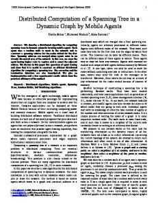
The current development of mobile and wireless technologies enables direct ad hoc communication between various kinds of mobile entities, such as vehicles, smartphones, terrestrian robots, flying robots, or satellites. In all these contexts, the set of communication links between entities (network topology) changes continuously. Not only changes are frequent, but in general they are unpredictable and can make the network partitioned at any time. Clearly, the usual assumption of connectivity does not hold here. Also, the classical view of a network whose dynamics corresponds to failures is no longer suitable in these scenarios, where dynamics is the norm rather than the exception. This shift in paradigm impacts algorithms and the definition of problems all together. What does it mean, for instance, to elect a leader in a partitioned network like the one in Figure 1? Is the objective to distinguish a unique global leader, whose leadership applies over time and space, or is it rather to maintain a unique leader in each connected component, deleting one when two components merge and creating one when a component splits? The same remark holds for spanning trees. Should an algorithm construct a unique, global tree whose logical edges survive network intermittence, or should it build and maintain a forest of trees, each of which spans an (as large as possible) part of the The Computer Journal,
network in a classical way? Both viewpoints make sense, and have been considered e.g. in [5, 13] (former interpretation) or [4, 12] (second interpretation).
FIGURE 1. Spanning forest in a sparse dynamic network.
In this paper, we focus on the second interpretation, illustrated in Figure 1, which reflects scenarios where the expected output of the algorithm should relate to the current configuration of the network (e.g. groups of robots or drones, each group having a spanning tree for coordination), through maintaining and updating the structure in order to match the underlying topology. This type of structure can then serve for communication within each group, and possibly be used by a higher level application (with the classical advantages that tree-like topologies offer regarding e.g. broadcast or Vol. ??,
No. ??,
????
2
1
routing. A specificity of this type of algorithms is that termination never occurs. More significantly, and perhaps differently to self-stabilization, it may happen that the execution never stabilizes (i.e., changes are too frequent to converge to a single tree per component), precluding approaches whereby the computation of a new solution requires the previous computation to have completed. The present work is an attempt at understanding what can still be computed (and guaranteed) in terms of spanning trees in such dynamic networks, with no assumptions as to the rate of change, their simultaneity, or global connectivity. In this seemingly chaotic context, we present an algorithm that strives to maintain as few trees per components as possible, while always guaranteeing key properties. 1.1.
Related work
Several works have addressed the spanning tree problem in dynamic networks, with different goals and assumptions. Burman and Kutten [9] and Kravchik and Kutten [16] consider a self-stabilizing approach where the legal state corresponds to having a (single) spanning tree and topological changes are the fault. The strategy consists in recomputing the entire tree when a change occurs. This general approach, sometimes called the “blast away” approach, is meaningful if stable periods of time exist, which is not the case in (unrestricted) highly dynamic networks. Note that selfstabilizing approaches do not deal only with topological changes; they also tolerate any initial configuration. In contrast, while the dynamics is arbitrary in our case, the processes are supposed to behave in correct ways and be properly initialized. Furthermore, in these settings, the network is generally connected, thus in absence of faults for sufficiently long, self-stabilization algorithms eventually build a single global spanning tree. A number of spanning tree algorithms use random walks for their elegance and simplicity, as well as for their inherent locality. In particular, approaches that involve multiple coalescing random walks allow for uniform initialization (each node starts in the same state) and topology independence (same strategy whatever the graph). Pionneering studies involving such processes include Bar-Ilan and Zernik [7] (for the problem of election and spanning tree), Israeli and Jalfon [15] (mutual exclusion), and Chapter 14 of Aldous and Fill [2] (general analysis). The principle of using coalescing random walks to build spanning trees in mildly dynamic networks was used by Baala et al. [6] and Abbas et al. [1], where tokens are annexing territories gradually by capturing each other. Regarding dynamicity, both algorithms require the nodes to know (an upper bound on) the cover time of the random walk, in order to regenerate a token if they have not been visited for
INTRODUCTION
some time. Besides the strength of this assumption (akin to knowing the number of nodes n, or the size of components in our case), the efficiency of the timeout approach decreases dramatically with the rate of topological changes. In particular, if they are more frequent than the cover time (itself in O(n3 )), then the tree is constantly fragmented into “dead” root-less (i.e. leader-less) pieces. Another algorithm based on random walks is proposed by Bernard et al. [8]. Here, the tree is constantly redefined as the token moves (in a way that reminds the snake game). Since the token moves only over present edges, those edges that have disappeared are naturally cleaned out of the tree as the walk proceeds. Hence, the algorithm can tolerate failure of the tree edges. However it still suffers from detecting the disappearance of tokens using timeouts based on the cover time, which as we have seen, suits only slow dynamics. A recent work by Awerbuch et al. [4] addresses the maintenance of minimum spanning trees in dynamic networks. The paper shows that a solution to the problem can be updated after a topological change using O(n) messages (and same time), while the O(m) messages of the “blast away” approach was thought to be optimal. (This demonstrates, incidentally, the revelance of updating a solution rather than recomputing it from scratch in the case of minimum spanning trees.) The algorithm has good properties for highly dynamic networks. For instance, it considers as natural the fact that components may split or merge perpetually. Furthermore, it tolerates new topological events while an ongoing update operation is executing. In this case, update operations are enqueued and consistently executed one after the other. While this mechanism allows for an arbitrary number of topological events at times, it still requires that such burst of changes are only episodical and that the network remains eventually stable for (at least) a linear amount of time in the number of nodes, in order for the update operations to complete and thus the logical tree to be consistent with physical reality. All the aforementioned algorithms either assume that global update operations (e.g. wave mechanisms) can be performed regularly, or that some node can collect global information about the tree structure. As far as dynamics is concerned, this forbids arbitrary and ever going changes to occur in the network. 1.2.
A high-level (graph-level) mechanism.
A high-level graph scheme for the maintenance of a (not necessarily minimum) spanning forest in unrestricted dynamic networks was proposed in [10], using a coarse grain interaction model inspired from graph relabeling systems [18] (bearing common features with so-called population protocols [3]). The algorithm was left without further analysis until [12], where its correctness
1.3
Our contribution.
3
was established and basic properties discussed in more details, however still considering the coarse-grain graphbased model. In the present article, this algorithm can be seen as a guiding principle, the main components of which – merging, circulation, and regeneration – are non-trivially adapted into a distributed message passing algorithm. The principle is as follows. Initially every node hosts a token and is the root of its own individual tree. Whenever two roots/tokens are located at both endpoints of a same edge (see merging rule on Figure 2), one of them is destroyed and the underlying node selects the other as parent: both trees (of arbitrary size) are merged locally and instantly. In absence of merging opportunity, the tokens execute a random walk within their own tree in the hope for (farther) merging opportunities (see circulation rule on Figure 2). As they circulate, the tokens flip (again, locally) the parentchild relations so that a directed path from any node in the tree towards its root is maintained. The fact that the random walk takes place within the tree (as opposed to the whole network) is crucial for this property. In fact, this simple feature is what enables to recover a consistent state immediately after an edge of the tree has disappeared. Indeed, it suffices for the child side of the lost edge to regenerate a new token/root, while being safe that no other node in the tree can do so (see regeneration rule on Figure 2). In conclusion, this scheme allows for all operations to be handled in a purely localized fashion (let apart global convergence).
(a) Merging rule
(b) Circulation rule
× (c) Regeneration rule
FIGURE 2. Spanning forest principle (high-level representation). Black nodes are those having a token. Black directed edges denote child-to-parent relationships. Gray vertical arrows represent transitions. The cross on the edge in (c) represents a loss of link (disconnection).
More precisely, at a graph level, this scheme guarantees that the network remains covered by a spanning forest at any time, in which 1) no cycle ever appears, 2) maximal subtrees always are directed rooted trees (with a token at the root), and 3) every node always belongs to such a tree, and so, whatever the rate and scale of topological changes. As to performance, analyzing it requires first to define what metric is relevant in this context. It is not expected that the rate of changes allows any algorithm to converge towards a single tree per connected component (which is, in a sense, the optimal state in such problem). Before
such concerns, a more important question remained to be answered as to whether such a mechanism could be implemented in more conventional message passing models. 1.3.
Our contribution.
We present the first adaptation of the above mechanism into the synchronous message passing model from [17]. Due to the loss of atomicity (in particular, the loss of exclusivity) in the interaction, the algorithm turns out to be much more sophisticated than its graph-level counterpart. While still reflecting the same abstract principle, it faces problems that require conceptual differences. In particular, the original model prevented (conveniently) a node to select a parent at the same time as it is itself selected as parent by another node, thereby making cycle avoidance straightforward. One of the ingredients in the new algorithm to circumvent this type of problem is an original technique (referred to as the unique score technique) that consists of maintaining, network-wide, a set of score variables that always remains a permutation of the set of nodes IDs. This mechanism allows us to break symmetry and avoid the formation of cycles in a context where IDs alone did not suffice. (We believe this technique is of independent interest.) The synchronicity in our model remains a significant restriction. However, one may consider the fact that, in addition to considering unrestricted dynamics, the transition from a coarse-grain abstract model to a distributed message passing model already induces an significant gap in difficulty, of both the description of the algorithm and its correctness analysis. The current work makes a step forward in the direction of even more realistic models, being possibly semisynchronous or asynchronous. The paper is organized as follows. In Section 2, we present the synchronous message passing model from [17], slightly adapted (in an equivalent way) and notations that we use throughout the paper. Then, Section 3 presents the algorithm, whose correctness analysis is developped through Section 4. Finally, Section 5 discusses some aspects related to performance that include preliminary experimental results, which can be seen as (partial) practical validation of our algorithm. 2.
MODEL AND NOTATIONS
The network is represented by a graph sequence G = (G1 , G2 , . . . ), such that Gi = (V, Ei ), where V is a fixed set of vertices and Ei is a dynamically changing set of undirected edges. (We indeed assume, for simplicity of the analysis, that nodes do not join or leave during execution. However, this is not a design limitation of the algorithm itself, which can deal with churn so long as new nodes are correctly initialized.) Following Kuhn et al. [17], we consider a synchronous (rounded)
4
3
computational model, where in each round i, the set of edges Ei determines which nodes communicate. At the beginning of each round, each node sends a message that was prepared at the end of the previous round. This message is sent to all its neighbors in Ei , although the list of these neighbors is a priori unknown to the node. Then, it receives all messages sent by its neighbors (in the same round), and finally computes its new state and its message for the next round. Due to the reciprocity of undirected links, a node can determine upon reception which nodes have received its own message. In summary, each round corresponds to three phases (send, receive, compute), which corresponds to a rotation of the original model of [17] where the phases are (compute, send, receive). This adaptation is not necessary, but makes the expression of our algorithm and of its correctness simpler. In particular, correctness predicates are satisfied by the end of each round (as opposed to the middle of each round if the original model had been used). The nodes possess unique identifiers which are nonnegative integers; in particular, for any two nodes u and v, it either holds that ID(u) > ID(v) or ID(u) < ID(v). A node can specify what neighbor its message is intended to (although all neighbors will receive it) by setting the target field of that message. Symmetrically, the ID of the emitter of a message can be read in the sender field of that message. Since the edges are undirected, if u receives a message from v at round i, then v also receives a message from u at round i. We call this property the principle of reciprocity. Globally, the progress of the execution is represented as a sequence of configurations (C0 , C1 , C2 , ..., Ci ), where each Ci captures the state of all nodes at the end of round i (except for C0 , the initial state). We use interchangeably the terminology “after round i” and “at/by the end of round i”, and similarly for “before round i” and “at the beginning of round i”. 3.
THE ALGORITHM
In this section, we present a message passing algorithm which adapts (“implements” in the theoretical sense) the spanning forest mechanism described in Section 1.2 into the synchronous model from [17]. We first describe the variables present at each node, then the structure of a message, and finally the algorithm itself with both an informal description and detailed listings of pseudocode. 3.1.
State variables
Besides the ID variable, which we assume is externally initialized, each node has a set of variables which reflects its situation in the tree: status accounts for the possession of a token (T if it has a token, N if it does not); parent contains the ID of this node’s parent
THE ALGORITHM
(⊥ if it has none); children contains the set of this node’s children (∅ if it has none). Observe that both variables status and parent are somewhat redundant, since in the spanning forest principle (see Section 1.2) the possession of a token is equivalent to being a root. Our algorithm enforces this equivalence, yet, keeping both variables separated simplifies the description of the algorithm and our ability to think of it intuitively. Variable neighbors contains the set of nodes from which a message was received in the last reception. These neighbors may or may not belong to the same tree as the current node. Variable contender contains the ID of a neighbor that the current node considers selecting as parent in the next round (or ⊥ if there is no such node). Finally, the variable score is the main ingredient of our cycle-avoidance mechanism, whose role is described below. 3.1.1. Initial values: All the nodes are uniformly initialized. They are initially the root of their own individual tree (i.e. status = T , parent = ⊥, and children = ∅). They know none of their neighbors (neighbors = ∅), have no contenders (contender = ⊥), and their score is set to their own ID. 3.2.
Structure of a message (and associated variables)
Messages are composed of a number of fields: sender is the ID of the sending node; status its status in the tree (either T or N); and score its score when the message was prepared. The field action is one of {F LIP, SELECT, HELLO}. Informally, SELECT messages are sent by a root node to another root node to signify that it “adopts” it as a parent (merging operation); F LIP messages are sent by a root node to circulate the token to one of its children (circulation operation); HELLO messages are sent by a node by default, when none of the other messages are sent, to make its presence and status known by its neighbors. Finally, target is the ID of the neighbor to which a FLIP or a SELECT message are intended (⊥ for HELLO messages). Received messages are stored in a variable mailbox, which is a map collection whose keys are the senders ID (i.e., a message whose sender ID is u can be accessed as mailbox[u]). In each round, the algorithm makes use of a RECEIVE() function that clears the mailbox and fill it with all the messages received in that round (one for each physical neighbor). A node can thus update the set of its neighbors by fetching the keys of its mailbox. Similarly, it can eliminate from its list of children those nodes which are no more neighbor. As mentioned above, every node prepares at the end of a round the message to be sent at the beginning of the next round. This message is stored in a variable outMessage. We allow the short hand m ← (a, b, c, d, e)
3.3
Description of the algorithm
to define a new message m whose emitter is node a (with status b and score e); target is node d; and action is c. 3.2.1. Initial values: The mailbox is initially empty (mailbox = ∅) and outMessage is initialized to the tuple (ID, T, HELLO, ⊥, ID). 3.3.
5 it sets its parent variable to u and its status to N (Lines 8 and 9). If the edge disappeared, then u does not receive the message, which is lost. However, due to the reciprocity of message exchange, v does not receive a message from u either and thus simply does not executes the corresponding changes. By the end of the round, either the trees are properly merged, or they are properly separated.
Description of the algorithm
The algorithm implements the general scheme presented in Section 1.2. In this section we explain how each of the three components (merging, circulation, regeneration) is implemented. Then we discuss the specificities of the merging operation in more details. In particular, the loss of atomicity in the message passing model makes this operation entangled with that of circulation. The resulting solution is substantially more sophisticated than its original scheme, and yet it faithfully reflects the same high-level principle. Let us start with some generalities. In each round, each node broadcasts to its neighbors a message containing, among others, its status (T or N) and an action (SELECT, FLIP, or HELLO). Whether or not the message is intended to a specific target (which is the case for SELECT and FLIP messages), all the nodes who receive it can possibly use this information for their own decisions. (In absence of SELECT or FLIP messages, recall that HELLO messages are sent to make such information always available.) More generally, based on the received information and the local state, each node computes at the end of the round its new status and the local structure of its tree (variables children and parent), then it prepares the next message to be sent. We now describe the three operations. Throughout the explanations, the reader is invited to refer to Figure 3, where an example of execution involving all of them is shown. The detailed algorithm is given in the listings of Algorithm 1, which uses functions defined in Algorithm 2. 3.3.1. Merging: If a root (i.e. a node having a token), say v, detects the existence of a neighbor root with higher score than its own, then it considers that node as a possible contender, i.e. as a node that it might select as a parent in the next round (Lines 18 to 20). The value of this score is recorded in a variable called contenderScore. If several such roots exist, then the one with highest score, say u, is chosen (through updating contenderScore every time a larger value is found). At the beginning of the next round, v sends a SELECT message to u (Line 24) to inform it that it is its new parent. Two cases are possible: either the considered edge is still present in that round, or it disappeared in-between both rounds. If it is still present, then u receives the message and adds v to its children list, among others (Line 16). As for v,
3.3.2. Circulation: If a root v does not detect another root with higher score, then it selects one of its children at random, if it has any (see Line 27), otherwise it simply remains root. Randomness is not a strict requirement of our algorithm; the random walk strategy could be replaced with other deterministic strategies (although with possible consequences on performance). Once the child is chosen, say u, the root prepares a FLIP message intended to u, and sends it at the beginning of the next round. Two cases are again possible, whether or not the edge {u, v} is still present in that round. If it is still present, then u receives the message, it updates its status and adds v to its children list, among others (Lines 15 and Line 16). As for v, it sets its parent variable to u and its status to N (Lines 8 and 9). If the edge disappeared, then v can detect it as before simply does not executes the corresponding changes. Node u, on the other hand, detects that the edge leading to its current parent disappeared, thus it regenerates a token (discussed next). Notice that in the absence of a merging opportunity, a node receiving the token in round i will immediately prepare a FLIP message to circulate the token in the next round. Unless the tree is composed of a single node, the tokens are thus moved in each round. In order for them to remain detectable in this case, the status announced in F LIP messages is T (whereas it is N for SELECT messages). 3.3.3. Regeneration: The first thing a non-root node does after receiving the messages of the current round is to check whether the edge leading to its current parent is still present. If the edge disappeared, then the node regenerates a root directly (Line 7), and only this node regenerates a token in the resulting tree. And if a tree is broken into several pieces simultaneously, then each of the resulting subtree will have exactly one node performing this operation. 3.3.4. The unique score technique: Unlike the high-level graph model from [12], in which the merging operation involves two nodes in an exclusive way, the non-atomic nature of message passing allows for a chain of selection with arbitrary many nodes (e.g. a selects b, b selects c, etc.). This has both advantages and drawbacks. One advantage is that it speeds up the initial merging process (see rounds 1 and 2 in Figure 3). On the other hand, these chains may create cycles,
6
4 4
←
s→
3
3
s 6
(a) End of initialization
f 1 ←
←
7
6
(c) End of round 2
4
(d) End of round 3
4 f→
1
7 ←f
2
5 6
8 3
7
7
3
3 2
2 8
←
f
7 5
5
8
6 (e) End of round 4
5
f→
×
8 5
6
(b) End of round 1
4
1
5
7←s
7 ←h→
2
f→
2
←
←
h→ ←
5
8
f
3
2 h→
2
4
s→
h→ ←
1
8
→
8
1
s→
f→
3
1 s→ 4 s
←h →
← h→
←h→
→ ←h
← h→
1 ←h→ 4
CORRECTNESS ANALYSIS
6
6
(f) End of round 5
(g) End of round 6
FIGURE 3. Example of execution of the algorithm with all types of operations: parent selection (s →, for SELECT), token circulation (f →, for FLIP), and tree disconnection (× ←). Hello messages are omitted for readability (except for Fig (a)); they are sent by default when no other message is sent (see Section 3.2). The displayed states are at the end of each round, showing messages to be sent at the beginning of next round. Black (resp. white) nodes are those (not) having a token (i.e. being roots). Tree edges are represented by bold directed arrows. Dashed edges are edges which have just disappeared.
Using IDs
Round 1
←F
CORRECTNESS ANALYSIS
2 1
F→
5 4
2 3 5
5
F→
3 1
4
(result) 2
4 2
3 1
i+1
←F
4
5
2 3 1
3 ←
5 S
1
4 2
S→
3
5
5
2
←
S
4
S→
1
4
4 2
3
This section establishes a number of properties about the spanning forest algorithm. In particular, we prove the claims regarding what property is always satisfied, regardless of the rate of changes. Because the proofs are technical, we provide first a preamble that includes
1
i
(result) 4.
Using Scores
5
S→
and they are the reasons why the score technique was introduced. Figure 4 shows an example of execution in which breaking ties based on IDs may create a cycle. Consider a chain of selection in round i + 1 that ends up at some root node u (here, ID 5). Nothing prevents u to have passed the token to a lower-ID child v (ID 1) in round i. Then, node v may select in round i + 1 a node (here, ID 2, of which it overheard a T -message in round i) which lies downstream a selection chain ending up at u, thereby creating a cycle. The score mechanism prevents such a situation by enforcing that after each FLIP, the new root has a larger score than its predecessor (see Lines 9 and 13 in Algorithm 2). The score mechanism also guarantees that the current set of scores (network-wide) is always a permutation of the initial set of scores. Hence, scores are always unique. All of these elements are crucial ingredients in the proofs of correctness (Section 4).
3
FIGURE 4. Example of use of the score technique (ID permutation). In the left scenario, the token is lost and a cycle is created, while this cannot happen.
4.1
Preamble and outline of the proof
7
Algorithm 1: Main Algorithm 1 2
repeat SEND(outMessage);
3
mailbox ← RECEIVE();
4
neighbors ← mailbox.keys(); children ← children ∩ neighbors
5
// Received messages, indexed by sender ID // All the senders IDs
// Regenerates a token if parent link is lost if status=N ∧ parent 6∈ neighbors then BECOME ROOT();
6 7
// Checks if the outgoing FLIP or SELECT (if any) was successful if outMessage.action ∈ {FLIP,SELECT} ∧ outMessage.target ∈ neighbors then ADOPT PARENT(outMessage)
8 9
// Processes the received messages contender ← ⊥; contenderScore ← 0; forall message ∈ mailbox do if message.target = ID then if message.action = FLIP then BECOME ROOT(); ADOPT CHILD(message); // called for both FLIP or SELECT else if message.status = T ∧ message.score > contenderScore then contender ← message.sender; contenderScore ← message.score; // Prepares the message to be sent
10 11 12 13 14 15 16 17 18 19 20
outMessage ← ⊥ if status = T then if contenderScore > score then PREPARE MESSAGE(SELECT, contender); else if children 6= ∅ then PREPARE MESSAGE(FLIP, random(children)); if outMessage = ⊥ then PREPARE MESSAGE(HELLO, ⊥)
21 22 23 24 25 26 27 28 29 30
;
a few helping definitions and a less technical outline of the proof. Then, the proof is described through two main parts called consistency and correctness, in reference to aspects defined in the preamble. 4.1.
Preamble and outline of the proof
We first define a handful of instrumental concepts that help minimize the number of properties to be proven. Then, as we start formulating the key properties to be proved, we adopt concise notations regarding the state of the system. Precisely, we denote by (i− )u.varname (resp. (i+ )u.varname) the value of variable varname at node u at the beginning (resp. at the end) of round i. (For concision, we use before and after [round i] with the same meaning.) Notice that for any node u, round i,
and variable varname, it holds that (i+ )u.varname = ((i + 1)− )u.varname. We use whichever notation is the most convenient in the given context. 4.1.1. Helping definitions These definitions are not specific to our algorithm, they are general graph concepts that simplify the subsequent proofs. Definition 4.1 (Pseudotree and pseudoforest). A directed graph whose vertices have outdegree at most 1 is a pseudoforest. A vertex whose outdegree is 0 is called a root. The weakly connected components of a pseudoforest are called pseudotrees. Lemma 4.1. A pseudotree has at most one root.
8
4 Algorithm 2: Functions called in Algorithm 1.
1 2 3
4 5 6 7 8 9
10 11 12 13
14 15 16 17
18 19
20 21
procedure BECOME ROOT status ← T; parent ← ⊥; procedure ADOPT PARENT(outMessage) status ← N; parent ← outMessage.target; if outMessage.action = FLIP then children ← childrenrparent; score ← min(score, mailbox[parent].score); procedure ADOPT CHILD(message) children ← children + message.ID; if message.action = FLIP then score ← max(score, message.score); procedure PREPARE MESSAGE(action, target) switch action do case SELECT do outMessage ← (ID, N, SELECT, target, score); case FLIP do outMessage ← (ID, T, FLIP, target, score); case HELLO do outMessage ← (ID, status, ⊥, ⊥, score);
Proof. By definition, a pseudotree T = (VT , ET ) is connected, thus |ET | ≥ |VT | − 1. If T has several roots, then at least two nodes in VT have no outgoing edge. Since the others have at most one, we must have |ET | ≤ |VT | − 2, which is a contradiction. Lemma 4.2. If a pseudotree T contains a root r, then it has no cycle. Proof. Let V1 ⊂ T be the set of nodes at distance 1 from V0 = {r}. Since r has outdegree 0, there is an edge from each node in V1 to r. Since T is a pseudotree, these nodes have no other outgoing edge than those ending up in V0 . The same argument can be applied inductively, all nodes at distance i having no other outgoing edges than those ending up in Vi−1 . Definition 4.2 (Correct tree and correct forest). At the light of Lemma 4.1 and 4.2, we define a correct tree (or simply a tree) as a pseudotree in which a root can be found. We naturally define a correct forest (or simply a forest) as a pseudoforest whose pseudotrees are trees. Finally, because forests are considered in a spanning context, we say that a pseudoforest F is a correct forest on graph G iff F is a correct forest and F is a subgraph of G. Defining correct trees as pseudotrees in which
CORRECTNESS ANALYSIS
a root can be found is the key. When the moment arrives, this will allow us to reduce the correctness of our algorithm to the presence of a root in each pseudotree. 4.1.2. Consistency At the end of a round, the state of an edge (whether it belongs to a tree, and if so, in what direction) must be consistently decided at both endpoints: Definition 4.3 (forest consistency). The configuration Ci is forest consistent if and only if for all nodes u, (i+ )u.parent = v ⇔ u ∈ (i+ )v.children. The proof of forest consistency is inductively established by Theorem 4.1, based on the consistency of the initial configuration (Lemma 4.3) and the maintenance of the consistency over the rounds (Lemma 4.18). Forest consistency allows us to reduce the output of interest of the algorithm after each round i to the mere parent variable. At the end of round i, the values of all parent variables should be consistent with the underlying graph Gi . Definition 4.4 (graph consistency). The configuration Ci is graph consistent if and only if for all nodes u, (i+ )u.parent = v ⇒ {u, v} ∈ Ei . This property is established by Corollary 4.1. Graph consistency allows us to say that the output of the algorithm forms a pseudoforest on Gi . Definition 4.5 (Resulting forest). Given a round i ≥ 1, occurring on graph Gi , the graph Fi = (V, EFi ) such that EFi = {(u, v) : {u, v} ∈ Ei , (i+ )u.parent = v} is called the pseudoforest resulting from round i. As explained in Section 3.1, the variables parent and status are somewhat redundant, since the possession of a token is synonymous with being a root. The equivalence between both variables after each round is established in Lemma 4.4 (state consistency). The main advantage of this equivalence is that it allows us to formulate and prove a large number of lemmas using either variable, depending on which is the most convenient in the given context. 4.1.3. Outline of the proof In this section, we prove that the resulting forest is always correct (Definition 4.2). To achieve that goal, we first define a validity criterion at the node level, which recursively ensures the correctness of the pseudotree this node belongs to thanks to Definition 4.2 (i.e. the existence of a root implies correctness). Definition 4.6. A node u is said to be valid at the beginning of round i if either (i− )u.status = T or (i− )u.parent is valid at the beginning of round i. The correctness of the whole forest can thus be established through showing that, first, it is initially
4.2
Consistency (detailed proofs)
correct (Lemma 4.3) and, second, if it is correct after round i, then it is correct after round i + 1 (Theorem 4.2). The latter is difficult to prove, and it involves a number of intermediate steps that correspond to a case analysis based on every action a node can perform (sending FLIP messages, SELECT messages, etc.). We say that u sends a FLIP (resp. SELECT) in round i if and only if (i− )u.outM essage.action = F LIP (resp. SELECT). We say that it sends it to node v if and only if (i− )u.outM essage.target = v. Finally the FLIP or SELECT is said to be successful (resp. unsuccessful) if {u, v} ∈ Ei (resp. {u, v} ∈ / Ei ). We first prove that a node u that sends a successful FLIP to v in a round, is valid at the end of that round (Lemma 4.23) because at the end of that round v is a root. The proof relies on the fact that during a given round, a node cannot receive a FLIP and send a SELECT or a FLIP (Lemma 4.20). We then prove some necessary properties on the score variable at each node. For instance, a node changes its score at most once during a round (Lemma 4.25 and 4.26). Also, the set of all scores are a permutation of the node identifiers after each round (Lemma 4.27). Then we prove that a node that sends a successful SELECT in a round i, is valid at the end of that round (Lemma 4.36). This part is the most technical and is the one that proves that chains of selection can not create cycles thanks to the property that score variables remain a permutation of all nodes IDs. Finally, we prove that all roots at the beginning of a round are still valid at the end of the round (Lemma 4.37). Therefore, if all nodes are valid at the beginning of round, then they are also valid at the end of the round (Theorem 4.2). Since they are initially valid (Lemma 4.3), we conclude by induction on the number of rounds. 4.2.
Consistency (detailed proofs)
Lemma 4.3. The configuration C0 is forest consistent and graph consistent. In C0 , the resulting pseudoforest is correct. Proof. The parent variable is initialized to ⊥ and u.children is empty for every node u. So, the configuration C0 is forest consistent and graph consistent. Furthermore, all initial pseudotrees are of the form Tu = ({u}, ∅); they contain a root (u itself) and are therefore correct trees. Lemma 4.4 (state consistency). For all round i, for all node u, (i+ )u.status = T ⇔ (i+ )u.parent = ⊥ Proof. Initially, at any node u, u.status = T and u.parent = ⊥. The change of u.status to N always comes with the assignment of a non-null identif ier (outM essage.target) to u.parent (procedure
9 ADOPT PARENT()), and assigning the value T to u.status is always followed by the change of u.parent to ⊥ (procedure BECOME ROOT()). So at any configuration, v.parent = ⊥ if and only if v.status = T . Lemma 4.5. If u does not send a FLIP or SELECT in round i, then u does not execute the procedure ADOPT PARENT() during round i. Proof. The execution of the procedure ADOPT PARENT() by u is conditioned by the sending of a SELECT or a FLIP by u during the current round (Line 8). Observation 1. Whenever a node u prepares its message to be sent during round i, we have u.parent = ((i − 1)+ )u.parent (resp. children, status). Lemma 4.6. If u sends a FLIP or SELECT in round i, then (i− )u.status = T . Proof. u sends in round i the message prepared in round i−1. If u sends a FLIP or a SELECT in round i then in round i − 1 PREPARE MESSAGE() is called with FLIP or SELECT as action (lines 24 or 27). Both instructions are conditioned by status = T . Lemma 4.7. If u sends a message containing T in round i, then (i− )u.status = T . Proof. The procedure PREPARE MESSAGE() is executed by a node u in round i − 1 to construct the message m to be sent in round i. In all cases PREPARE MESSAGE() sets m.status to T only if u.status = T . Lemma 4.8. If u sends a SELECT to v in round i, then (i− )u.score < ((i − 1)− )v.score. Proof. The value of the score field in the message sent by a node v in round i − 1 is ((i − 1)− )v.score. Assumes that the node u sends a SELECT to v in a round i. So, during round i − 1, u sets its contender variable to v and its contenderScore variable to message.score, message being the message sent by v at the begining of round i − 1. From that time to the end of round i − 1, u.score is not modified. So (i− )u.score < ((i − 1)− )v.score, if u sends a SELECT to v in a round i. Lemma 4.9. If at the beginning of round i, the configuration is forest consistent then only (i− )u.parent can send a FLIP to u during round i. Proof. A node v can prepare a FLIP message to the node u at the end of round i − 1 only if u ∈ (i− )v.children. We have (i− )u.parent = v according to the hypothesis (forest consistency at the beginning of round). Therefore, only the node (i− )u.parent can prepare a FLIP message to node u, at the end of round i − 1.
10
4
4.2.1. Graph consistency: Lemma 4.10. Let u be a node such that (i− )u.parent 6= v ∧ (i+ )u.parent = v. Then u sends a successful FLIP or SELECT to v during round i. Proof. The only change of parent by u to a non-null identifier v in a round i is at the execution of the procedure ADOPT PARENT() which is conditioned by the reception of a message from v (Line 9). If u receives the message of v during round i then v effectively receives the message sent by u (reciprocal reception property). Lemma 4.11. Let u be a node such that (i− )u.parent = v ∧ (i+ )u.parent = v. We have {u, v} ∈ Ei . Proof. By Lemma 4.4, we have (i− )u.status = N. So, u does not send a FLIP or SELECT during round i (Lemma 4.6). Then, u does not execute ADOPT PARENT() during round i according to Lemma 4.5. Since (i+ )u.parent = v we conclude that u does not execute the procedure BECOME ROOT() during round i. So u did receive a message from (i− )u.parent in round i. We have {u, v} ∈ Ei . Corollary 4.1 (graph consistency). Every configuration is graph consistent. Proof. The configuration reached after any round is graph consistent (Lemmas 4.10 and 4.11). 4.2.2. Forest consistency: Lemma 4.12. If (i− )u.parent = + (i )u.parent = v or (i+ )u.parent = ⊥.
v
then
Proof. According to Lemma 4.4, we have (i− )u.status = N , so u cannot send a FLIP or a SELECT in round i (by Lemma 4.6). Therefore, u does not execute ADOPT PARENT() in round i (Lemma 4.5). We conclude that (i+ )u.parent = v or (i+ )u.parent = ⊥.
CORRECTNESS ANALYSIS
in round i, u changes u.parent to v then u ∈ (i+ )v.children: (i− )u.parent 6= v ∧(i+ )u.parent = v ⇒ u ∈ (i+ )v.children. Proof. u sets u.parent to v only if the FLIP or SELECT was successful (Lemma 4.10). Therefore v has received the FLIP or SELECT message sent by u. The addition of a node u to v.children by v is done during the excution of the procedure ADOPT CHILD() which is conditioned by the reception of a FLIP or a SELECT message mu from u (mu .target = v, Line 16). The procedure ADOPT CHILD() is executed after Line 5 which is the only instruction that could remove u from v.children. So, u ∈ (i+ )v.children. We have (i− )u.parent 6= v ∧ (i+ )u.parent = v ⇒ u ∈ (i+ )v.children. Lemma 4.15. Assume that at the beginning of round i, the configuration is forest consistent. If in round i, v adds u to v.children then (i+ )u.parent = v: u 6∈ (i− )v.children ∧ u ∈ (i+ )v.children ⇒ (i+ )u.parent = v. Proof. v adds u to v.children only if it excutes the procedure ADOPT CHILD() which is conditioned by the reception of a FLIP or a SELECT sent by u. As the reception of messages is reciprocal, u also receives in round i a message from v. This satisfies the condition for u to execute the procedure ADOPT PARENT() which sets u.parent to v. Only the execution of BECOME ROOT() (at line 15) could modify the value of u.parent. This procedure would be executed only if u has received a FLIP during round i which cannot be the case. Notice that u does not receive a FLIP during round i (Lemma 4.13). Lemma 4.16. Assume that at the beginning of round i, the configuration is forest consistent. If in round i, u changes u.parent from v to another value then u 6∈ (i+ )v.children: (i− )u.parent = v ∧ (i+ )u.parent 6= v ⇒ u 6∈ (i+ )v.children.
Proof. We will establish the contraposition of the lemma statement: if u sends a FLIP or a SELECT in round i, then it does not receive a FLIP in round i. By Lemma 4.6, we have (i− )u.status = T . According to Lemma 4.4, (i− )u.parent = ⊥. Thus according to the hypothesis (forest consistency at the beginning of the round), for any node v, u ∈ / (i− )v.children. Therefore no node has prepared a FLIP message destined to u, in round i − 1 (Lemma 4.9). So u cannot receive a FLIP in round i.
Proof. If u changes (i+ )u.parent then we have (i+ )u.parent = ⊥ (Lemma 4.12). Only the execution of BECOME ROOT() by u sets u.parent to ⊥. The procedure BECOME ROOT() is executed in two cases: at the detection of a disconnection (Line 7), and at the reception of a FLIP message (Line 15). In the first case, the reciprocal reception property ensures that v does not receive the message sent by u. So, v removes u from children (Line 5). In the second case, u receives a FLIP from (i− )u.parent (Lemma 4.9). According to the reciprocal reception property, v receives the message sent by u during round i. So, v executes ADOPT PARENT((i− )v.outM essage) which removes u (i.e. (i− )v.outM essage.target) from v.children (Line 9).
Lemma 4.14. Assume that at the beginning of round i, the configuration is forest consistent. If
Lemma 4.17. Assume that at the beginning of round i, the configuration is forest consistent. If
Lemma 4.13. Assume that at the beginning of round i, the configuration is forest consistent. If u receives a FLIP in round i, then it does not send a FLIP nor a SELECT in round i.
4.3
Correctness (detailed proofs)
in round i, v removes u from v.children then (i+ )u.parent 6= v: u ∈ (i− )v.children ∧ u 6∈ (i+ )v.children ⇒ (i+ )u.parent 6= v. Proof. v removes u from v.children in two cases: at the detection of a disconnection (v does not receive a message from u, line 5), and when v executes (ADOPT PARENT((i).v.outM essage), line 9) In the first case, the reciprocal reception property ensures that u does not receive the message sent by v during round i. So, u becomes a root: it executes the procedure BECOME ROOT() (Line 7). In the second case, v executes So v did send ADOPT PARENT((i).v.outM essage). a successful FLIP or SELECT (Lemma 4.5). As v removes u from v.children during the execution of ADOPT PARENT((i).v.outM essage), we have (i− ).v.outM essage.target = u and (i− ).v.outM essage.action = F LIP (see the procedure ADOPT PARENT(outM essage)). So v sends a successful FLIP to u during round i. Therefore, in round i, u executes the procedure BECOME ROOT() (Line 15): u sets u.parent to ⊥. Lemma 4.18 (Forest Consistency). Let i be a round starting from a forest consistent configuration. The configuration reached at the end of round i is forest consistent Proof. The configuration after the round i is forest consistent according to Lemmas 4.14, 4.15, 4.16, 4.17. Notice that in the case where u does not change the value of its parent variable (resp. u stays in v.children) during round i, at the end of round i the forest consistency property is preserved according to the contraposition of Lemma 4.17 (resp. contraposition of Lemma 4.16) and the hypothesis. Theorem 4.1 (Consistency). Every configuration is forest consistent. Proof. C0 is forest consistent (Lemma 4.3). The configuration reached after any round is forest consistent (Lemma 4.18). 4.3.
Correctness (detailed proofs)
4.3.1.
Correctness of the resulting forest after token circulation: Lemma 4.19. Let v be a node. Only (i− )v.parent can send a FLIP to node v during round i. Proof. At the beginning of round i, the configuration is forest consistent (Theorem 4.1). Therefore, only the node (i− )v.parent can prepare a FLIP message to node v, at the end of round i − 1 (Lemma 4.9). Lemma 4.20. If u receives a FLIP in round i, then it does not send a FLIP nor a SELECT in round i. Proof. At the beginning of round i, the configuration is forest consistent (Theorem 4.1). Therefore no node
11 has prepared a FLIP message to node u, in round i − 1 (Lemma 4.13). Lemma 4.21 (Adoption). If u sends a successful FLIP or SELECT to v in round i, then (i+ )u.status = N and (i+ )u.parent = v. Proof. In round i, u.outM essage.action = F LIP or SELECT and v ∈ (i+ )u.neighbors. During round i, u executes the procedure ADOPT PARENT() (Line 9) which sets (i+ )u.parent to v. According to Lemma 4.20, u did not receive any FLIP message during round i. Only an execution of BECOME ROOT() by u at line 15 can change the value of u.parent during round i. This line is not executed during round i. Lemma 4.22. If u sends a successful FLIP to v, then (i+ )v.status = T . Proof. v received a message from u in round i, so {u, v} ∈ Ei . v executes the procedure BECOME ROOT() that changes v.status to T . After the execution of line 9, no instruction can set v.status to N until the end of round i. So (i+ )v.status = T . Lemma 4.23. If u sends a successful FLIP in round i, then u is valid after round i. Proof. By Lemmas 4.21 and 4.22 u’s parent has a status T after round i. 4.3.2. Proofs on score permutations: Lemma 4.24. If u sends a successful FLIP to v, then (i− )u.score ≤ (i+ )v.score. Proof. u sent a message mu to v at the beginning of round i such that mu.action = FLIP, mu.target = v.ID and mu.score = (i− )u.score. v received mu in round i, so {u, v} ∈ Ei . v executes the procedure ADOPT CHILD(mu) at line 16 in round i. This procedure sets the current score of v to max(v.score, mu.score), as mu.score = (i− )u.score. After the execution of this instruction, we have mu.score = (i− )u.score ≤ v.score. We notice that after this operation, no instruction can change the value of v.score during this round (Lemma 4.19). Lemma 4.25. (i− )u.score = (i+ )u.score unless u sends or receives a successful FLIP in round i. Proof. u changes its score value only by executing ADOPT PARENT(mu ) or ADOPT CHILD(mu ). Both instructions that changes u.score value in these procedures (Algorithm 2, line 9, 16) are conditioned by mu .action = F LIP . Lemma 4.26. A node u changes u.score at most once during a round. Proof. A node sends at most one FLIP message during a round. A node receives at most one FLIP message during a round (Lemma 4.19). Either a node receives a FLIP, sends one, or it does not receive and does not
12 send a FLIP during a given round (Lemma 4.20). So, according to Lemma 4.25, a node changes u.score at most once during a round. Lemma 4.27. Before each round, the set of scores is a permutation of the set of identifiers. Proof. After the initialization in each node u, u.score = u.ID. A node u changes its score only by executing ADOPT PARENT() or ADOPT CHILD(). We will do a proof by induction. We assume at the beginning of round i, the set of scores is a a permutation of the set of indentifiers. We have for any node u, mu.score = (i− )u.score. According to Lemma 4.25, only a node sending or receiving a successful FLIP may change its score value. Assume that the node u changes its score value during round i. Without lost of generality, we assume u sends the successful FLIP to a node v in round i. By hypothesis, u changes its score to (i− )v.score during the execution of ADOPT PARENT() in round i. We have (i− )u.score ≥ (i− )v.score. v executes the procedure ADOPT CHILD(mu) at line 16 in round i. This procedure sets the current score of v to max(v.score, mu.score), as mu.score = (i− )u.score. After the execution of this instruction, we have v.score = (i− )u.score (Lemma 4.24). According Lemma 4.26, we have (i+ )v.score = − (i )u.score and (i+ )u.score = (i− )v.score. 4.3.3.
Correctness of the resulting forest after mergings: In lemmas 4.31 and 4.32, we establish that if u sends a successful SELECT to v in round i either (i− )v.status = T or (i− )v.parent.status = T . In the first case, we have (i− )u.score < (i− )v.score, and in the second case, we have (i− )u.score < (i− )v.parent.score. Let ch be a series of nodes u0 , u1 , u2 such that (i+ )uj .parent = uj+1 and such that u0 sends a successful SELECT to u1 during round i. As a ch’s subchain of nodes having strictly increasing scores at the beginning of round i may be built: ch has no loops. So ch ends by a node having a token: all nodes on that chain are valid. Lemma 4.28. If v sends a message containing T in round i and (i+ )v.status = N , let w = (i+ )v.parent, then (i+ )w.status = T . Proof. If v sends a message containing T in round i, then (i− )v.status = T . If (i+ )v.status = N , then v has executed ADOPT PARENT() in round i, because it is the only procedure that sets v.status to N . v executes ADOPT PARENT() only if it has sent a FLIP message mv to a node w (mv .action 6= SELECT because mv .status = T ), and if w has received the message mv (reciprocal reception property). At the reception of mv by w, w executes BECOME ROOT() (Line 16) which sets w.status to T and from this line until the end of
4
CORRECTNESS ANALYSIS
the round no instruction can change w.status to N . So (i+ )w.status = T . At the execution of ADOPT PARENT() by v, v sets v.parent to w. After this instruction there is only BECOME ROOT() that can modify the value of v.parent, and it is conditioned by the reception of a FLIP message. According to Lemma 4.20 v cannot call BECOME ROOT() because it cannot receive a FLIP message. So w = (i+ )v.parent. So, if v sends a message containing T in round i and (i+ )v.status = N , and w = (i+ )v.parent, then (i+ )w.status = T . Lemma 4.29. If v sends a message containing T in round i and (i+ )v.status = N , let u = (i+ )v.parent, then (i+ )u.score ≥ (i− )v.score. Proof. We have (i− )v.status = T because in round i − 1, v.status cannot be modified after the execution of PREPARE MESSAGE(). If (i− )v.children 6= ∅ then v sends a FLIP message in round i to one of its children u. Then, either {u, v} ∈ Ei and (i+ )v.parent = u, (i+ )u.status = T and (i+ )u.score ≥ (i− )v.score (see Lemmas 4.22 and 4.24); or (i+ )v.status = T . Lemma 4.30. If u sends a successful SELECT to v in round i then ((i − 1)− )v.status = T . Proof. Node u prepared a SELECT message to v in round i − 1, thus it had u.contender = v, which implies it received from v a message containing T . We have then ((i − 1)− )v.status = T because after the execution of PREPERE MESSAGE() by v in round i − 2, v.status cannot be changed. Lemma 4.31. If u sends a successful SELECT to v in round i and (i− )v.status = T , then (i− )u.score < (i− )v.score. Proof. Lemma 4.30 implies that ((i−1)− )v.status = T . By Lemma 4.8, the sending of the SELECT implies that (i− )u.score < ((i − 1)− )v.score and Lemma 4.25 implies in turn that ((i − 1)− )v.score = (i− )v.score, which yields the inequality. (Lemma 4.25 says that the score of v could have only changed if v sent or received a successful FLIP in round i − 1, which was not the case for reception since ((i − 1)− )v.status = T (Lemme 4.19, nor for emission since (i− )v.status = T (Lemma 4.21).) Lemma 4.32. If u sends a successful SELECT to v in round i and (i− )v.status = N , then let w = (i− )v.parent. It holds that (i− )w.status = T and (i− )u.score < (i− )w.score. Proof. By Lemma 4.30 we have ((i−1)− )v.status = T . Furthermore, the fact that v is considered as a contender implies that v sent a message containing T in round i − 1. Then, Lemmas 4.8 and 4.29 respectively imply that (i− )u.score < ((i − 1)− )v.score and ((i − 1)− )v.score ≤ (i− )w.score. Lemma 4.28 implies that (i− )w.status = T .
13 Lemma 4.33 (Cancellation). If u sends a failed FLIP or SELECT in round i, then (i+ )u.status = T . Proof. By Lemma 4.6, we have (i− )u.status = T . v did not receive the message from u implies that {u, v} ∈ / Ei . So, in round i, v ∈ / u.neighbors (u did not receive the message from v). Only during the execution of ADOPT PARENT(), called in line 9, u can change its status to N . This procedure is not executed during round i. Lemma 4.34 (Conservation). If (i− )u.status = T and u does not send a FLIP or SELECT in round i, then (i+ )u.status = T . Proof. By Lemma 4.5, u does not execute the procedure ADOPT PARENT() during round i. u can set status variable to N only if it executes ADOPT PARENT(). Lemma 4.35. If (i− )u.status = T and u does not send a successful SELECT in round i, then u is valid after the round i. Proof. According to Lemma 4.23, after the successful sending of a FLIP message in round i, u is valid at the end of round i. If u sends a failed SELECT or a failed FLIP then u is valid after the round i by Lemma 4.33. otherwise, u did not send a SELECT or a FLIP during the round: it is also valid at the end of the round by Lemma 4.34. Lemma 4.36. If a node sends a successful SELECT in round i, then it is valid at the end of round i. Proof. Let S be the set of nodes that send a successful SELECT in round i and are not valid at the end of round i. We will prove, by contradiction, that S is empty. Assume S is non-empty and consider the node in S that had the largest score at the beginning of the round (say, node u). Such a node exists by Lemma 4.27. We will prove that u is valid after the round, which is a contradiction. Let v be the recipient of u’s successful SELECT. By Lemma 4.21 (i+ )u.parent = v, thus it is enough to show that v is valid after round i to get our contradiction. Let us examine both cases whether (i− )v.state = T or N . If (i− )v.status = T , then either v also sends a successful SELECT in round i, or it does not. If it does not, then it is valid after round i (Lemma 4.35). If it does, then it must be valid otherwise u is not maximal in S (Lemma 4.31). If (i− )v.status = N , then let w = (i− )v.parent. Two cases are considered, whether {v, w} ∈ Ei or not. If {v, w} ∈ / Ei then (i+ )v.status = T because the condition forces v to call the procedure BECOME ROOT() in Line 7 which makes it take the status T . After this, v can take the status N only during the execution of the procedure ADOPT PARENT() in Line 9. This procedure is called by v only if it sends a FLIP or a SELECT at the beginning of round i by Lemma 4.5. By Lemma 4.6, this cannot happen. Thus v is valid after round i. If
{v, w} ∈ Ei , we use the fact that (i− )w.status = T (Lemma 4.28, applicable because if u sends a SELECT to v in round i, then v’s message in round i−1 contained a T , otherwise v would not be considered as a contender by u.) in order to apply the same idea as we did above: either w also sends a successful SELECT in round i, or it does not. If it does not, then it is valid after round i (Lemma 4.35). If it does, then it must be valid otherwise u is not maximal in S (Lemma 4.32). 4.3.4. Correctness of resulting forest: Lemma 4.37. If (i− )u.status = T then u is valid after round i. Proof. According to Lemma 4.36, after the successful sending of a SELECT message in round i, u is valid at the end of round i. According to Lemma 4.23, after the successful sending of a FLIP message in round i, u is valid at the end of round i. If u sends a failed SELECT or a failed FLIP then u is valid after the round by Lemma 4.33. In otherwise, u is also valid the round by Lemma 4.34.
Theorem 4.2 (Resulting forest correctness). If all nodes are valid at the beginning of round i, then all nodes are valid after round i. Proof. Assume that a node v is invalid after round i. According to Lemma 4.37, (i− )v.status = N . Let u0 , u1 , u2 , ..., uk be the finite series of nodes such that for j ∈ [0, k − 1], (i− )uj .parent = uj+1 , (i− )uk .status = T , and u0 = v. This series exists because v is valid at the beginning of round i. Let u01 , u02 , ..., be the infinite series of nodes such that for all j ≥ 1 (i+ )u0j .parent = uj+1 , and (i+ )v.parent = u01 . This series exists because v is invalid (by hypothesis). According to Lemma 4.12, j ∈ [1, k], uj = u0j . According to Lemma 4.37, uk is valid. So all nodes of the series u0 , u1 , u2 , ..., uk are valid. There is a contradiction. 5.
DISCUSSION ABOUT PERFORMANCE
Our main focus in this paper is to present the spanning forest algorithm and prove that it guarantees a number of key properties, whatever the dynamics. Somewhat ironically, the same properties are satisfied even if the algorithm does nothing beyond initialization: every node remains forever a single-node tree, which satisfies all the predicates. Naturally, one expects more from an algorithm, in particular regarding convergence and performance. We offer here a preliminary discussion on these topics, starting with the quality metric to be used in such contexts and how our algorithm behaves in this respect.
14
5
5.1.
How to measure performance?
Since the network may always be partitioned, the natural way to define an optimal (at least, irreductible) state of our algorithm is that every connected component is covered by a single tree. However, if the rate of topological changes is high, then it may simply be impossible for an algorithm (however good) to converge towards such an optimal state in-between the changes. Completion time does not make sense either since this type of algorithms never terminate. In this context, a reasonable metric seems to be rather the number of trees per connected component, e.g. averaged over the execution or characterized in a stationary regime (for stochastic models of dynamic networks). This being said, if the network were to stabilize, then one would indeed hope that a single tree spans each component. Both aspects are now discussed. 5.2.
scale on the left side). The average ratio between both (i.e. the metric of interest, as discussed in Section 5.1) is depicted on the lower curves of the same Figures (using the scale on the right side). Every point of these curves corresponds to an average over 100 executions.
Convergence in case of network stability
At an abstract level, the spanning forest algorithm presented in this paper relies on random walks in trees. Since trees are bipartite graphs, it may so happen that two tokens never meet (at both extremities of a common edge) even if their respective trees offer merging opportunities. Standard techniques exist for preventing periodic walks, such as stopping the tokens occasionally (also called lazy walks). This variant is easy to incorporate in the existing algorithm, by having a node decide whether or not circulating the token (FLIP messages) with some probability. Apart from this, markov chain theory tells us that if the graph does not change, eventually all tokens in each component will merge leaving a single tree per component. 5.3.
DISCUSSION ABOUT PERFORMANCE
A practical scenario
We verified the applicability of our algorithm in a real world scenario. The algorithm was implemented1 using the JBotSim library [11] and tested against the Infocomm06 dataset [19]. This well known dataset is a record of the communication links among devices given to 78 people during the Infocomm conference in 2006. The update rate for the links is every 120 seconds, which means that the presence time of an edge is a multiple of 120 seconds, a somewhat optimistic granularity. In order to use these traces, one must decide how many rounds (of our computational model) can effectively be performed each second. We chose pessimistic options to counterbalance the coarse granularity of edge presence, namely either 10 rounds per second (mildly pessimistic) or 1 round per second (very pessimistic). For each, we measured the evolution of the number of connected components versus the number of trees resulting from the execution of our algorithm (upper curves on Figures 5 and 6, using the 1 The
source code of our algorithm is available upon request.
FIGURE 5. Number of roots (trees) versus number of connected components, assuming 10 rounds per second. The lower curves show the resulting ratio. (Infocomm06 dataset on 78 nodes.)
In summary, the number of trees per connected component is often close to 1 (1.027 in average in the first case, and 1.080 in the second case). Furthermore, the algorithm achieves an optimal configuration of a single spanning tree per connected component about 47% of the time in the first case (32.68% in the second case), which implies that the algorithm may be relevant in (at least some) practical scenarios. In fact, these traces correspond to a rather sparse scenario. The number of trees ranges from 10 to 70, on top of 78 nodes, which corresponds to trees whose average size ranges from 1.1 to 7.8 depending on the moment. Small trees are profitable to token-based algorithms in general and ours as a particular case. However, this setting is neither unrealistic nor uncommon, as sparseness is a typical feature of delay-tolerant networks (i.e. partitioned networks which are connected only over time and space), an important sub-class of highlydynamic networks. 5.4.
Additional remarks
This section proposed an initial discussion about performance. It is by no mean comprehensive and the performance evaluation of our algorithm remains essentially open, both experimentally and theoretically. On the experimental side, it would be interesting to consider scenarios (data sets) with various scales of density and stability. On the theoretical side, the process at play here is one of coalescing random walks
5.4
Additional remarks
15
[6]
[7]
[8]
[9]
FIGURE 6. Number of roots (trees) versus number of connected components, assuming 10 rounds per second. The lower curves show the resulting ratio. (Infocomm06 dataset on 78 nodes.)
[10]
[11]
over dynamic graphs. These processes are known to be difficult to analyse even in static graphs (see e.g. [14]), and restricting the walks to trees adds even more dependency in the analysis. In this paper, we introduced the first message passing algorithm for maintaining spanning forests under unrestricted dynamics. Both the algorithm and its correctness are significantly more sophisticated than their coarsegrain analogues. A deeper performance analysis that combines both experimental and theoretical aspects is considered for future works.
[12]
[13]
ACKNOWLEDGMENT
[14]
This work was partially supported by ANR projects ESTATE (ANR-16-CE25-0009-03) and DESCARTES (ANR16-CE40-0023).
[15]
REFERENCES [1]
[2] [3]
[4]
[5]
Abbas, S., Mosbah, M., and Zemmari, A. (2006). Distributed computation of a spanning tree in a dynamic graph by mobile agents. In Proc. of IEEE Int. Conference on Engineering of Intelligent Systems (ICEIS), pages 1–6. Aldous, D. and Fill, J. (2002). Reversible markov chains and random walks on graphs. Berkeley Press. Angluin, D., Aspnes, J., Diamadi, Z., Fischer, M. J., and Peralta, R. (2006). Computation in networks of passively mobile finite-state sensors. Distributed Computing, 18(4):235–253. Awerbuch, B., Cidon, I., and Kutten, S. (2008). Optimal maintenance of a spanning tree. J. ACM, 55(4):18:1–18:45. Awerbuch, B. and Even, S. (1984). Efficient and reliable broadcast is achievable in an eventually
[16]
[17]
[18]
[19]
connected network. In Proceedings of the third annual ACM symposium on Principles of distributed computing, pages 278–281. ACM. Baala, H., Flauzac, O., Gaber, J., Bui, M., and ElGhazawi, T. (2003). A self-stabilizing distributed algorithm for spanning tree construction in wireless ad hoc networks. Journal of Parallel and Distributed Computing, 63:97–104. Bar-Ilan, J. and Zernik, D. (1989). Random leaders and random spanning trees. In Workshop on Distributed Algorithms (WDAG), vol. 392 of LNCS, pages 1–12. Springer Berlin Heidelberg. Bernard, T., Bui, A., and Sohier, D. (2013). Universal adaptive self-stabilizing traversal scheme: Random walk and reloading wave. J. Parallel Distrib. Comput., 73(2):137–149. Burman, J. and Kutten, S. (2007). Time optimal asynchronous self-stabilizing spanning tree. In Pelc, A., editor, Distributed Computing, vol. 4731 of LNCS, pages 92–107. Springer Berlin Heidelberg. Casteigts, A. (2006). Model driven capabilities of the DA-GRS model. In Proc. of 1st Intl. Conference on Autonomic and Autonomous Systems (ICAS), pages 24–32. IEEE. Casteigts, A. (2015). JBotSim: a tool for fast prototyping of distributed algorithms in dynamic networks. In Proceedings of the 8nd international ICST conference on simulation tools and techniques (SIMUTools). Casteigts, A., Chaumette, S., Guinand, F., and Pign´e, Y. (2013). Distributed maintenance of anytime available spanning trees in dynamic networks. In Proceedings of 12th conf. on Adhoc, Mobile, and Wireless Networks (ADHOC-NOW), vol. 7960 of LNCS. Casteigts, A., Flocchini, P., Mans, B., and Santoro, N. (2015). Shortest, fastest, and foremost broadcast in dynamic networks. Int. Journal of Foundations of Computer Science, 26(4):499-522. Cooper, C., Elsasser, R., Ono, H., and Radzik, T. (2013). Coalescing random walks and voting on connected graphs. SIAM Journal on Discrete Mathematics, 27(4):1748–1758. Israeli, A. and Jalfon, M. (1990). Token management schemes and random walks yield self-stabilizing mutual exclusion. In Proceedings of the ninth annual ACM symposium on Principles of distributed computing, pages 119–131. ACM. Kravchik, A. and Kutten, S. (2013). Time optimal synchronous self stabilizing spanning tree. In Afek, Y., editor, Distributed Computing, vol. 8205 of LNCS, pages 91–105. Springer Berlin Heidelberg. Kuhn, F., Lynch, N., and Oshman, R. (2010). Distributed computation in dynamic networks. In Proceedings of the 42nd ACM symposium on Theory of computing (STOC), pages 513–522. ACM. Litovsky, I., Metivier, Y., and Sopena, E. (2001). Graph relabelling systems and distributed algorithms. In Handbook of graph grammars and computing by graph transformation. Citeseer. Scott, J., Gass, R., Crowcroft, J., Hui, P., Diot, C., and Chaintreau, A. (2006). Crawdad trace cambridge/haggle/imote/infocom (v. 2006-01-31).