Maintaining Simultaneously Consistent Views of a ... - CiteSeerX

Maintaining Simultaneously Consistent Views of a Distributed System using Common Knowledge Tal Mizrahi

Maintaining Simultaneously Consistent Views of a Distributed System using Common Knowledge Research Thesis Submitted in Partial Fulfillment of the Requirements for the Degree of Master of Science in Electrical Engineering

Tal Mizrahi

Submitted to the Senate of the Technion - Israel Institute of Technology

Elul, 5766

Haifa

September, 2006

This Research Thesis Was Done Under The Supervision of A/Prof. Yoram Moses in the Department of Electrical Engineering

Acknowledgement I would like to express my uttermost gratitude to my advisor, A/Prof. Yoram Moses, for his devoted guidance throughout this research. His vision and extraordinary intuition have inspired me in my work. My warm thanks to my parents, Tsipi and Joe, for their encouragement and support, to my brother, Amit, for all the LaTeX tips, and of course to my lovely wife, Hagit, for putting up with me during these long years in the Technion.

The Generous Financial Assistance of the Technion is Gratefully Acknowledged.

Contents

1

2

3

Abstract

1

List of Symbols and Abbreviations

3

Introduction

7

1.1

Motivation . . . . . . . . . . . . . . . . . . . . . . . . . . . . . . . . .

7

1.2

Previous Work . . . . . . . . . . . . . . . . . . . . . . . . . . . . . . .

8

1.3

Research Goals . . . . . . . . . . . . . . . . . . . . . . . . . . . . . .

8

1.4

Outline . . . . . . . . . . . . . . . . . . . . . . . . . . . . . . . . . .

10

Preliminaries

11

2.1

The Communication Network . . . . . . . . . . . . . . . . . . . . . .

11

2.2

Nature’s Role: Inputs and Failures . . . . . . . . . . . . . . . . . . . .

12

2.3

Full-Information Protocols . . . . . . . . . . . . . . . . . . . . . . . .

14

2.4

Definition of the Continuous Consensus Problem . . . . . . . . . . . .

15

2.5

Systems and Knowledge . . . . . . . . . . . . . . . . . . . . . . . . .

16

2.6

Common Knowledge . . . . . . . . . . . . . . . . . . . . . . . . . . .

19

Solving Continuous Consensus

21

3.1

The CC Problem . . . . . . . . . . . . . . . . . . . . . . . . . . . . .

21

Clean Rounds . . . . . . . . . . . . . . . . . . . . . . . . . . . . . . .

21

A Simple Protocol for Continuous Consensus . . . . . . . . . . . . . .

24

Good and Bad Processes . . . . . . . . . . . . . . . . . . . . . . . . .

26

4

5

The Core . . . . . . . . . . . . . . . . . . . . . . . . . . . . . . . . .

28

The Horizon . . . . . . . . . . . . . . . . . . . . . . . . . . . . . . . .

30

C ON C ON . . . . . . . . . . . . . . . . . . . . . . . . . . . . . . . . .

31

3.2

Continuous Consensus and Common Knowledge . . . . . . . . . . . .

36

3.3

Waste and C ON C ON . . . . . . . . . . . . . . . . . . . . . . . . . . .

44

Waste . . . . . . . . . . . . . . . . . . . . . . . . . . . . . . . . . . .

44

A Generalized Definition of Waste . . . . . . . . . . . . . . . . . . . .

46

3.4

Clean Rounds Revisited . . . . . . . . . . . . . . . . . . . . . . . . . .

51

3.5

A Run of C ON C ON . . . . . . . . . . . . . . . . . . . . . . . . . . . .

54

The horizon Revisited . . . . . . . . . . . . . . . . . . . . . . . . . . .

54

Critical Times Revisited . . . . . . . . . . . . . . . . . . . . . . . . .

55

Good and Bad Processes Revisited . . . . . . . . . . . . . . . . . . . .

56

Local Waste and Destination . . . . . . . . . . . . . . . . . . . . . . .

57

Uniform Continuous Consensus

61

4.1

The UCC Problem . . . . . . . . . . . . . . . . . . . . . . . . . . . .

61

A protocol for UCC . . . . . . . . . . . . . . . . . . . . . . . . . . . .

62

Conclusion

65

5.1

Summary of Results . . . . . . . . . . . . . . . . . . . . . . . . . . . .

65

5.2

Future Work . . . . . . . . . . . . . . . . . . . . . . . . . . . . . . . .

68

A Detailed Proofs

73

A.1 Optimality of C ON C ON Revisited . . . . . . . . . . . . . . . . . . . .

73

A.2 Correctness proofs for U NI C ON C ON . . . . . . . . . . . . . . . . . . .

74

List of Figures 2.1

An execution graph and i’s view Vi (k + 1). . . . . . . . . . . . . . . . .

14

3.1

The S IMPLE CC protocol for process i. . . . . . . . . . . . . . . . . . .

24

3.2

Illustration of the S IMPLE CC Protocol. . . . . . . . . . . . . . . . . .

25

3.3

Sets Gi (k) & Bi (k) are based on Vi (k + 1). . . . . . . . . . . . . . . . .

29

3.4

The core computed at time k. . . . . . . . . . . . . . . . . . . . . . . .

30

3.5

The C ON C ON protocol for process i. . . . . . . . . . . . . . . . . . . .

32

3.6

An instance of Moses and Tuttle’s fixed-point construction by i at time m. 40

3.7

The Horizon vs. k in a run r. . . . . . . . . . . . . . . . . . . . . . . .

55

3.8

Critical time vs. k in a run r. . . . . . . . . . . . . . . . . . . . . . . .

56

3.9

Gi (k) and Bi (k) in r. . . . . . . . . . . . . . . . . . . . . . . . . . . . .

57

3.10 desti (k) and horizoni (k) in r. . . . . . . . . . . . . . . . . . . . . . . .

58

3.11 Local Waste . . . . . . . . . . . . . . . . . . . . . . . . . . . . . . . .

60

4.1

64

Process x’s computation in U NI C ON C ON. . . . . . . . . . . . . . . . .

Abstract

In a distributed system it is often necessary for all processes to maintain a consistent view of the world. However, the existence of communication failures in a system may prevent processes from obtaining a consistent view. Continuous consensus is the problem of having each process i maintain at each time k an up-to-date core Mi [k] of information about the past, so that the cores at all processes are guaranteed to be identical. Our analysis assumes an unreliable synchronous system, with an upper bound of t failures. The notion of continuous consensus enables a new perspective on classical problems such as the consensus or the Simultaneous Byzantine Agreement (SBA) problems, and allows for simpler analysis. A simple algorithm for continuous consensus in fault-prone systems with crash and sending omission failures called C ON C ON is presented, based on a knowledge-based analysis. Continuous consensus is shown to be closely related to common knowledge. Via this connection, the characterization of common knowledge by Moses and Tuttle is used to prove that C ON C ON is optimal—it produces the largest possible core at any given time. Finally, a second algorithm is presented that provides an optimum uniform solution to continuous consensus, in which all processes (faulty and nonfaulty) maintain the same core information at any given time.

Abstract [1]

2

List of Symbols and Abbreviations A(r, m)

The set of active processes at (r, m).

Bi (k)

Set of bad processes computed by i at time k + 1.

bi (k)

Number of bad processes computed by i at time k + 1.

β

Labelling function - determines which messages are successful.

C

Common knowledge among all processes.

CN

Common knowledge among the nonfaulty process.

c

Short for criti (k).

DS ϕ

Distributed knowledge of ϕ among the processes in S.

d(r, k)

The difference between N (r, k) and k (used in the computation of waste).

(m)

di

(k)

The difference between N

(m) i (k)

and k − m.

desti (m)

The destination of i at time m.

E

Edges of the communication graph.

ES ϕ

Everyone in the set S knows ϕ.

E

Set of monitored events.

E (V)

The set of monitored external inputs determined by the view V.

e

An event or an external input.

F`

Set of potentially faulty processes in `th iteration of the fixed-point construction.

Fˆ

The fixed-point of F` .

FIP

Full Information Protocol.

List of Symbols and Abbreviations fm

Failure model.

Gi (k)

Set of good processes computed by i at time k + 1.

g

A good process.

h

Index of the last iteration in the fixed-point construction.

horizoni (k)

The horizon of i at time k.

I

Set of possible input assignments in the system.

i

Process name.

j

Process name.

Ki ϕ

Process i knows ϕ.

k

Time / round counter.

kˆ

The final time in the fixed-point construction.

κ


L

Logical language.

Latesti [k]

Process i’s estimation of the critical time for k in C ON C ON.

Latestxu [k]

Process x’s estimation of the critical time for k in U NI C ON C ON.

`


`w

The round in which the waste is reached.

`lw

The round in which the local waste is reached.

λ

The empty view.

Mi [k]

The core of i at time k.

MiC [m]

Process i’s core according to C ON C ON.

Mxu [k]

Process x’s core according to U NI C ON C ON.

m


N

The set of nonfaulty processes.

4


N (r, k) (m) i (k)

N

5

The number of failures discovered up to round k. Number of failures discovered by i between rounds m and k.

n

Number of processes in the system.

P

Set of processes in the system.

P

Protocol.

Φ

The set of primitive propositions in the logical language.

ΦE

The set of primitive propositions confined to facts about external inputs.

ϕ

Fact or proposition.

R

System.

r

Run.

S`

Set of potentially nonfaulty processes in `th iteration of the fixed-point construction.

Sˆ

The fixed-point of S` .

Σi

Set of initial local states of i.

t

Upper bound on the number of failures in the system.

V

Set of nodes in the communication graph.

Vi (m)

View of process i at time m (subgraph of V ).

W (r)

The waste or r.

(m)

Wi

(k)

The local waste at time k w.r.t time m.

X

Contents of the core.

x

An arbitrary (possibly faulty) process.

z

An arbitrary (possibly faulty) process.

ζ

Input assignment function - assigns an input from E to every point.


6

Chapter 1 Introduction 1.1

Motivation

Maintaining consistency of the information held by different nodes in an unreliable distributed system is a challenging problem. Whether it is a system whose nodes share resources, or a system in which critical decisions are made according to the most recent data at hand, it is highly important to maintain consistency of the nodes’ information. A core of identical information maintained at different sites allows decisions performed in a distributed manner to be compatible with each other. Moreover, with the rapid growth of the internet over the last two decades, distributed systems operations are no longer restricted to being internal. In many cases, external elements interact concurrently with different nodes of the system. This places a stronger emphasis on the need to present a consistent view to the world at different nodes at a given time. A core of information that is guaranteed to be identical at all sites at any given time, and contains as much information as possible, is a very desirable tool in implementing such a consistent view. This thesis deals with the design of efficient protocols for maintaining such a core. The challenge, however, is that different nodes in a distributed system typically have asymmetric information. Part of this information—the facts that are common knowledge—is identical for all agents and, moreover, can in principle be identified by each agent. By acting on information that is common knowledge, agents are guaranteed

1. Introduction

8

to be acting on consistent information available to all agents.

1.2

Previous Work

The role of common knowledge for consistent simultaneous actions has been firmly established in the literature [2, 3, 4, 5]. Dwork and Moses [3] presented an optimal1 solution to simultaneous Byzantine agreement in the presence of crash failures, by using the notions of clean rounds and waste. They proved that simultaneous agreement can be reached exactly when the value of at least one agent’s initial vote becomes common knowledge. Moses and Tuttle [4] extended this work to the more complex (sending) omission failure model, and presented optimal solutions for a broader class of simultaneous choice problems. Implicit in the latter work is the computation of a core of information that characterizes the common knowledge at any given point in time. This computation is based on a subtle fixed-point construction. Providing an up-to-date consistent picture of the system at different sites can sometimes alleviate the need to explicitly activate voting or agreement protocols to handle individual transactions (see, for example, [6]). Weaker guarantees than simultaneous consistency are popular, where consistency is guaranteed over time: If one process can determine that an event has occurred, the others will eventually know this as well [7]. These weaker consistency conditions are essential in some systems since simultaneous coordination requires nontrivial common knowledge, and this is not attainable in truly asynchronous systems [2].

1.3

Research Goals

The current work introduces the continuous consensus problem, in which a core Mi [k] of information is continuously maintained at every correct process i in the system. All 1 Throughout

this work we use the term optimal referring to the time it takes to reach agreement or

consensus, rather than the computation complexity.

1. Introduction

9

local copies of the core must be identical at all times k, and every interesting event from a set of possible events, E , should eventually enter the core. The continuous consensus problem is studied in synchronous systems with crash and omission failures. We assume an upper bound of t failures in every run of our system. We shall show that the analysis of continuous consensus (CC for short) shown in this work allows for a simple and elegant solution to the problem of maintaining simultaneously consistent views in the system. The continuous consensus problem generalizes many problems having to do with simultaneous coordination. For example, in the distributed firing squad problem [8], the system may receive an alarm message from the outside world. If a correct process receives such a message, then it is required that at some later point all correct processes “fire” simultaneously. In addition, “firing” is not allowed to occur in different rounds by different processes (hence in a non-simultaneous fashion), nor is it allowed to take place in a run before an alarm message has been received in the system. Clearly, if the arrival of an alarm message is a monitored event in a continuous consensus protocol, then the presence of an alarm in the shared core can be used as a necessary and sufficient condition for firing. Continuous consensus can also be used as a generalization of simultaneous versions of Byzantine agreement and the consensus problem (cf. [3]), as well as for the class of simultaneous choice problems of [4]. In this work we present an algorithm called C ON C ON that solves the CC problem. C ON C ON is optimal in providing at any given time the largest and most informative core possible. The algorithm will provide the most up-to-date consistent picture of the system, without the need to explicitly activate voting or agreement protocols to handle individual transactions. A variant of the CC problem, which we call uniform continuous consensus (UCC), requires that the core be consistent among all processes in the systems, rather than just among the correct ones. We present U NI C ON C ON, which is a variant of C ON C ON that solves the UCC problem. Our solutions to CC and UCC rely on a knowledge-based analysis. A close connec-

1. Introduction

10

tion is shown between continuous consensus and common knowledge: it is shown that the core of shared information, Mi [k] is common knowledge among the correct processes at time k. Moreover, the optimality of C ON C ON is proven using the characterization of common knowledge in the crash and omission failure models given in [4]. Our analysis also aims at extending Dwork and Moses’ analysis of clean rounds and waste [3] to the more complicated omission model.

1.4

Outline

This work is organized as follows. Chapter 2 provides a formal definition of our system, and some technical background to the notions described in later chapters. Chapter 3, which is the heart of this work, presents the continuous consensus problem and its solution, C ON C ON, as well as proving its correctness and optimality. Chapter 4 describes the uniform continuous consensus problem, and introduces U NI C ON C ON. Finally, a few concluding remarks are presented in Chapter 5. Some of the detailed proofs are given in Appendix A.

Chapter 2 Preliminaries Our treatment of the continuous consensus problem will be driven by a knowledge-based analysis. A general approach to modelling knowledge in distributed systems was initiated in [2] and given a detailed foundation in [5] (most relevant to the current work are Chapters 4 and 6). The lion’s share of technical analysis in this thesis will be performed with respect to a single protocol, which gives rise to a specific class of systems. For ease of exposition, our definitions will be tailored to this particular setting.

2.1

The Communication Network

We consider a synchronous network with n ≥ 2 possibly unreliable processes, denoted by P = {1, 2, . . . , n}. Each pair of processes is connected by a two-way communication link. Processes correctly identify the sender of every message they receive. They share a discrete global clock that starts out at time 0 and advances by increments of one. Communication in the system proceeds in a sequence of rounds, with round k + 1 taking place between time k and time k + 1. Each process starts in some initial state at time 0. Then, in every following round, the process first sends a set of messages to other processes, and then receives messages sent to it by other processes during the same round. In addition, a process may also receive requests for service from clients external to the system (think, for example, of deposits and withdrawals at branches of a bank), or input from sensors with information about the world outside of the system (e.g., smoke detec-

2. Preliminaries

12

tors). Finally, the process may perform local computations based on the messages it has received. The history of an infinite execution of such a network will be called a run.

2.2

Nature’s Role: Inputs and Failures

We think of a solution to the continuous consensus problem as a protocol operating (or playing) against an adversary called nature. Nature determines two central aspects of any given run: inputs and failures.

Inputs.

We consider a setting in which every process starts out in an initial local state

from some set Σi , and can receive an external input in any given round k (this input is considered as arriving at time k). The initial local state of each process can be thought of as its external input at time 0. We represent the external inputs in an infinite execution as follows. Define a set V = P × N of process-time nodes (or nodes, for short). An (external) input assignment is a function ζ associating with every (initial) node hi, 0i at time 0 an initial state from Σi and with each node hi, ki an input from a set of possible inputs, I . Our analysis is independent of the type or structures of the elements of I .

Failures. The second aspect of a run that is determined by nature is the identity of the faulty processes, and the details of their faulty behavior. These depend on the particular failure model being assumed. In this thesis we consider two closely-related failure models, called the crash model and the sending omission model, which is a generalization of the crash model. For simplicity, a process will be considered faulty in a run if it displays faulty behavior at any point during the run. In the crash failure model, a faulty process crashes in some round k ≥ 1. In this case, it behaves correctly in the first k − 1 rounds and sends no messages from round k + 1 on. During its crashing round k, the process may succeed in sending messages on an arbitrary subset of its channels. In the sending omission model (or the omission model for short), a faulty process may omit to send messages in any given round. It sends messages only according to its protocol (it cannot

2. Preliminaries

13

misrepresent or lie), and nature determines for every round what subset of its messages will successfully be delivered. We remark that even faulty processes receive all messages sent to them over non-blocked channels. If a message is not delivered, its sender is necessarily faulty. We formally represent the failure pattern in a given run via an edge-labelled graph (V, E, β), where V is the set of process-time nodes defined above, and E = {(hi, ki, h j, k + 1i) : i 6= j, k ≥ 0}. An edge e = (hi, ki, h j, k + 1i) ∈ E stands for the round k + 1 communication in the channel from i to j. The labelling function β : E → {Y, N} captures when such channels are blocked and when they operate correctly. Intuitively, β(e) = N means that e is blocked for communication, while β(e) = Y means that it is not blocked. In the latter case, a message on e, if sent, will be delivered. Nature’s combined contribution to a run r is captured by an execution graph. This is a labelled graph Gr = (V, E, ζ, β) with labels ζ on the vertices giving the input assignment and labels β on the edges defining the failure pattern.1 Notice that all execution graphs over n processes have the same edge and vertex sets (V, E)— a complete grid of n × N nodes, with edges from each node u ∈ V at level k to all nodes of level k + 1 with a process name different from u’s. Different execution graphs G differ only in the labelling functions ζ and β. Figure 2.1 contains an illustration of the nodes of an execution graph, with some of the edges describing round k + 1. Observe that all edges from one time point to the next are in the graph—some are crossed, depicting their being blocked by β, while the others are available for communication. We now consider particular subgraphs of G = (V, E, ζ, β) that will be useful later on. Given a node u = hi, mi ∈ V , we denote by Vu the set of nodes containing the nodes hi, `i ∈ V for all ` ≤ m as well as all nodes u0 = h j, ki ∈ V such that there is a directed path of edges of E from u0 to u , in which all edges are labelled ‘Y’ . Intuitively, Vu contains all nodes about which u has potentially received information either directly or via a sequence of messages. We define the maximal potential view (or view for short) at node u = hi, mi in G, denoted by Vi (m), to be the subgraph of G generated by Vu , i.e., 1 The

run r appears in the superscript of Gr . Throughout the thesis, we omit explicit reference to the

run whenever it is clear from context.

2. Preliminaries

14

Vi (m) = (V 0 , E 0 , ζ0 , β0 ) = (Vu , E Vu , ζ Vu , β E 0 ). See Figure 2.1 for an illustration of a view Vi (m). The view VS (k) of a set S ⊆ P of processes at a time k is defined to be the union of the graphs V j (k), over all j ∈ S. We say that a view V is contained in a view V0 if the nodes of V are a subset of those in V0 , and V is the subgraph of V0 generated by these nodes. Thus, every node in V has the same external input as in V0 , and for every pair of nodes in V, they are connected by an edge in V exactly if they are connected by one in V0 . In some cases, it will be convenient to talk about views VS (k) at a time k < 0. The view in this case is denoted by λ. It is called an empty view, and is contained in every possible view VS0 (k0 ). …

1

…

|

i

… … Vi (k + 1) …

|

…

…

…

…

…

〈i, k +1〉

|

…

n

0

1

…

k

k+1

Figure 2.1: An execution graph and i’s view Vi (k + 1).

2.3

Full-Information Protocols

A full-information protocol (FIP) is one in which processes have perfect recall and observe all incoming messages and external inputs that they receive. Moreover, in every round, every process sends a message encoding all of its information to all other processes. It is not hard to show that in any such protocol a process is able to reconstruct Vi (k) from its information at time k. Without loss of generality, we will assume for the

2. Preliminaries

15

sake of concreteness that the local state of a process is maintained in the form of a view Vi (k), and the message sent by i in round k + 1 is Vi (k). Since in a FIP a message is sent on every channel in every round, the execution graph describes all aspects of a run: i.e., what inputs are received by the processes, which processes are faulty, and, for every message, whether or not it is delivered. Moreover, the contents of delivered messages can also be derived from the graph G. From now on we shall identify a run r of a

FIP

with its execution graph Gr . Since a run of

FIP

is

determined by the inputs and failures, we sometimes denote such a run by r = FIP(ζ, β). It is a folk theorem, perhaps first proven formally in a fault-prone setting by Coan [9], that any deterministic protocol can be simulated by a FIP. Using a FIP as we defined it above may be quite inefficient in terms of communication complexity. However, in practice a

FIP

may be implemented quite efficiently (see,

for example, [5]). Further discussion of the communication complexity of the FIP in our context appears in Section 3.1.

2.4

Definition of the Continuous Consensus Problem

We now specify the continuous consensus problem formally. With respect to a set E of monitored events, we would like each process i to hold a copy of a shared list of events of E . An event is defined based on the messages delivered in the run, and on initial states and external inputs that processes have received (and the times at which they were received). The precise definition of E will depend on the application. We define a continuous consensus (CC) service to be a distributed protocol that at all times k ≥ 0 provides each process i with a core Mi [k] of events of E . In every run of this protocol the following properties are required to hold, for all nonfaulty processes i and j. Accuracy: All events in Mi [k] occurred in the run. Consistency: Mi [k] = M j [k] at all times k.

2. Preliminaries

16

Completeness: If an event e ∈ E is known to process j at any point, then e ∈ Mi [k] must hold at some time k. The consistency property guarantees that the information in the local lists is in fact shared among the nonfaulty processes at any given time. Since an event is in Mi [k] for some nonfaulty process i only if it is also in M j [k] for all other nonfaulty processes j, it follows that a process i may know of the occurrence of a monitored event e ∈ E long before e is in Mi [k]. In many cases it is, of course, desirable to have the shared list in a continuous consensus application be as up-to-date as possible. A variant of this problem, which we call uniform continuous consensus (UCC), is defined similarly, but Accuracy and Consistency should hold for arbitrary processes and not just for nonfaulty ones. Completeness, however, is still restricted to events that are known to nonfaulty processes: If an event e ∈ E is known to a nonfaulty process j at any point, then e ∈ Mi [k] must hold (for all processes i, of course) at some time k.

2.5

Systems and Knowledge

Generally speaking, we identify a system with a set R of runs. For a general protocol, a run r is an infinite sequence of states, and there is a well defined local state ri (m) for every process i and time m. For the

FIP

we identify runs with execution graphs, while

in general every execution graph will determine a run of a protocol P (cf. [4, 5]). The systems that we study in this thesis are thus parameterized by a tuple (n,t, fm, I ), where n ≥ 2 is the number of processes, t is a bound on the number of faulty processes in a run (where t ≤ n − 2), fm ∈ {crash, omission} is a failure model, and I is a nonempty set of (external) input assignments. The exact identity and internal structure of I are application-dependent. A FIP system R = R(n,t, fm, I ) is defined to be the set of all runs of the FIP with n processes, at most t of which fail according to the failure model fm, and where initial states and external inputs conform to one of the input assignments in I . Our definitions imply that, in a precise sense, the inputs in a

FIP

system R are independent

from the failures that occur (and hence carry no information about them): If there are

2. Preliminaries

17

runs r, r0 ∈ R where r = FIP(ζ, β) and r0 = FIP(ζ0 , β0 ), then R will also contain the run r00 = (ζ0 , β).2 Our analysis makes use of the knowledge that processes achieve at different times in various runs. As is standard in the literature, formulas will be considered true or false at a point, which is a pair (r, m) consisting of a run r ∈ R and a time m ∈ N. Moreover, since what is known at a point (r, m) may depend on what is true at other points, we define truth with respect to a system R. Let Φ = {p, q, p0 , . . .} be a set of propositions. Intuitively, a proposition is a basic primitive fact. An example of a relevant proposition in the context of continuous consensus is “ζ(i, k) = e”, stating the arrival of an external input e ∈ I at a given process i at time k. Given a system R, each proposition p ∈ Φ is identified with a set [[p]] of points of R. A proposition p ∈ Φ holds at (r, m), which we denote by (R, r, m) |= p, if (r, m) ∈ [[p]]. For simplicity, we identify the set of monitored events E with a subset ΦE ⊆ Φ, and restrict monitored events to depend only on the external inputs in the current run. Thus, if q ∈ ΦE then, for all input assignments ζ and runs r = FIP(ζ, β) and r0 = FIP(ζ, β0 ), and times m, we will have that (R, r, m) |= q iff (R, r0 , m) |= q. The core maintained by a continuous consensus algorithm consists of a set X ⊆ ΦE at any given time. We note that in our context the truth value of every q ∈ ΦE is independent of the time, m. Thus, in a given system, R, the truth value of q depends only on the run, r. We say that an event q has occurred in a run r if (R, r, m) |= q for all m ≥ 0. The core constructed by our proposed protocols will consist of the monitored events that are determined by a particular view computed at any given point. In order to describe such cores more formally, we denote

E (V) , {q ∈ ΦE : (R, r, m) |= q for all points (r, m) whose execution graph contains V}. 2 Recall

that the input assignments in I establishes the initial states of processes as well as the external

inputs they receive. Often, initial states may be independent of external inputs, and the inputs at one process may be independent of those at another. But our definitions do not require such independence. There could be strong correlation among inputs in I . Our definitions only imply that inputs carry no information about failures and vice-versa.

2. Preliminaries

18

Notice that E is monotone: If V is contained in V0 , then E (V) ⊆ E (V0 ). We construct a logical language L by closing Φ under Boolean connectives ∧ and ¬, and under modal knowledge operators Ki , DS , ES , C and CN where i ∈ P and S ⊆ P is a set of processes. Here Ki stands for process i’s knowledge, DS corresponds to the distributed knowledge that is implicit in the set of processes S, ES refers to facts known to every process in S, C stands for common knowledge, and CN stands for common knowledge among the nonfaulty processes. The semantics of the Boolean operators is standard; we now review the definitions for Ki and DS . Common knowledge and “everyone knows” are defined in the next subsection. The formal definitions (cf. [5]) of satisfaction for knowledge and distributed knowledge formulas are briefly stated as follows:

(R, r, m) |= Ki ϕ iff (R, r0 , m0 ) |= ϕ for all(r0 , m0 ) such that r0 ∈ R and ri (m) = ri0 (m0 ).

(2.1)

(R, r, m) |= DS ϕ iff (R, r0 , m0 ) |= ϕ for all (r0 , m0 ) such that r0 ∈ R and r j (m) = r0j (m0 ) for all j ∈ S. (2.2)

A process knows ϕ by this definition if its local state (which captures the information it has access to) implies that ϕ holds. Distributed knowledge is defined similarly, but is based on the combined information available to the members of a set S of processes. In a full-information protocol, the distributed knowledge of S is equivalent to the knowledge of a process whose local state at a point (r, m) of R is the view VSr (m). Knowledge in the FIP has a number of useful properties. For example, suppose that process i receives messages in round k + 1 from the processes in the set S. Then, by construction, VS (k) is contained in i’s view Vi (k + 1) at the end of the round. As a result, all facts about the past that are distributed knowledge of S at time k are known by i at time k + 1. This observation plays a role in the solution to the continuous consensus problem described in the next section.

2. Preliminaries

2.6

19

Common Knowledge

We define ES ϕ or “everyone in S knows ϕ” as follows: ES ϕ ,

^

Ki (ϕ)

(2.3)

i∈S

The formula CS ϕ is true if everyone in S knows ϕ, everyone in S knows that everyone m−1 ϕ. Thus common knowledge in S knows ϕ, etc. Define ES1 ϕ , ES ϕ, and E m S ϕ , ES E S

of ϕ among the processes in S, denoted CS ϕ, is defined as the infinite conjunction of ESm : CS ϕ , ϕ ∧ ES ϕ ∧ ES ES ϕ ∧ · · · ∧ E m S ϕ∧···

(2.4)

Specifically, we have an interest in two particular cases: S = N, or S = P. We denote common knowledge among the nonfaulty processes by CN . CP stands for common knowledge among all the processes in our system, and is denoted C for short. We present an equivalent semantic definition of satisfaction for CN , which will be more useful in the context of our analysis. Rather than defining common knowledge as an infinite conjunction of “everyone knows”, we define it in term of N-reachability.3 We say that two points (r, m) and (r0 , m) are N-neighbors, and write (r0 , m) ∼N (r, m), if there is some process j that is nonfaulty in both r and r0 for which r0j (m) = r j (m). In this case we say that the points (r, m) and (r0 , m) are indistinguishable by j. The “∼N ” relation is also called the similarity relation. The point (r0 , m) is N-reachable from (r, m) in R, if there is a finite sequence of points (r, m) = (r0 , m), (r1 , m), . . . , (rk , m) = (r0 , m) such that (r` , m) ∼N (r`+1 , m) holds for every 0 ≤ ` < k. Thus, N-reachability is the transitive closure of the ∼N relation. Moreover, it is an equivalence relation that defines a partition over the points of a system R. Common knowledge among the nonfaulty processes is then formalized by: 3 The

fact that in our systems a process can always distinguish between points (r, m) and (r0 , m0 ) with

m 6= m0 simplifies the definitions here slightly.

2. Preliminaries

20

(R, r, m) |= CN ϕ iff (R, r0 , m) |= ϕ for all points (r0 , m) that are N-reachable from (r, m) in R

(2.5)

A formal proof for the equivalence of the two definitions of common knowledge, in Equations 2.4 and 2.5 may be found in [5]. In other words, a fact ϕ is common knowledge among the processes in N at a point (r, m) if ϕ is valid in all the points that are N-reachable from (r, m). Very similarly, we can define common knowledge among all processes, C, by replacing the N in the definition of CN by P, the set of all processes in the system. More precisely, we say that the point (r0 , m) is reachable from (r, m) in R if there is a finite sequence of points of R (r, m) = (r0 , m), (r1 , m), . . . , (rk , m) = (r0 , m) such that for every 0 ≤ ` < k there is some j = j` for which r`j (m) = r`+1 j (m). Then (R, r, m) |= Cϕ iff

(R, r0 , m)

|= ϕ for all points (r0 , m) that are reachable from (r, m) in R

(2.6)

Chapter 3 Solving Continuous Consensus 3.1

The CC Problem

The continuous consensus problem was formally defined in Section 2.4. In this section we present our solution to this problem, which is the C ON C ON algorithm. We start by presenting a simple protocol which solves the CC problem, after which we present C ON C ON and prove its correctness. In the following subsection we provide some background which enables us to present the S IMPLE algorithm immediately afterwards.

Clean Rounds As mentioned in the introduction, the concept of clean rounds played a critical role in the analysis of Simultaneous Byzantine Agreement (SBA) by Dwork and Moses [3] in the crash model. In this model, a round of communication is clean if no new failure is discovered in the round. Following a clean round, all processes can have the same information about the past. Once it is common knowledge that a round was clean, the information available to nonfaulty processes before this round becomes common knowledge. We shall now present a formal definition of clean rounds. We define the set of Active processes in (r, k), denoted A(r, k), as the set of processes

3. Solving Continuous Consensus

22

that did not fail in the first k rounds of r.1 We say that the failure of process p is discovered in round k of r if k is the first time at which p’s faulty behavior is distributed knowledge, i.e., k is the first time at which (r, k) |= D(“p is f aulty”) holds. In this context D(·) refers to distributed knowledge among the active processes, i.e., DA(r,k) (·). Formally, a clean round is a round in which no process failure is discovered by the active processes. A round which is not clean is referred to as dirty. Notice that it is possible that the failure of a process p will be discovered in round k (which is thus a dirty round), whereas some of the processes may learn of p’s failure in round k + 1. Even so, if no other failures are discovered in round k + 1, it is a clean round, since p’s failure was discovered in round k. An important property of a clean round, presented in [3], is the following: If round k of r is clean, then every fact of which there is distributed knowledge in k − 1, becomes known to everyone at the end of round k. It is an inherent property of the crash failure model, that in a round in which process p fails, it may successfully send information to any subset of the other processes. As a result, information sent by p in round k may be known to some of the processes in k, and not known to others. On the other hand, the importance of clean rounds lies in the fact that all active processes successfully send their messages, and thus at the end of this round they have consistent views of the system. This property is phrased in the following theorem. Theorem 3.1 (Dwork and Moses) Let (r, k − 1) |= D ϕ. If round k of r is clean, then (r, k) |= E ϕ. Once again, by E ϕ we mean everyone among the active processes knows ϕ. We say that a fact ϕ is a fact about the initial configuration of the run r if its truth value is uniquely determined by the set of initial states Σ in r. Similarly, we say that a fact ϕ is about the first m rounds of r if its truth depends on the first m rounds of r. An 1 The

set of nonfaulty processes in the run is a subset of the active processes at time k. While the term

nonfaulty refers to the entire run, the term active refers to a specific time, and thus a process j who is active at time k may crash at some later time, and is thus considered faulty in the run.


23

important connection between clean rounds and common knowledge is presented in a theorem which was shown in [3] and is quoted below: Theorem 3.2 (Dwork and Moses) Let clean be the fact “a clean round has occurred”, and let ϕ be a fact about the initial configuration. If (r, k) |= C (clean) then (r, k) |= D ϕ i f f (r, k) |= C ϕ The theorem implies that once it becomes common knowledge that a clean round has occurred between times 0 and k, all information about the initial configuration becomes common knowledge. A direct corollary of Theorem 3.2 generalizes the result, and shows that if the appearance of a clean round in the time interval [m, k] is common knowledge at time k, then all information about the first m rounds becomes common knowledge. Corollary 3.3 Let ϕ be a fact about the first m rounds. Let clean(m, k) be the fact “a clean round occurred between times m and k”. If (r, k) |= C (clean(m, k)) then (r, k) |= D ϕ i f f (r, k) |= C ϕ Theorem 3.2 is a key tool in the characterization of common knowledge in [3]. However, while the definition of clean rounds, as well as the theorem, are valid in the crash model, the (sending) omission failure model is significantly more complex, since information about failures can be kept by faulty processes for a long while without reaching nonfaulty processes. Such information can then be delivered to nonfaulty processes only much later. Thus, in the omission model the information about failures evolves in a much more erratic fashion. Hence in the omission model clean rounds no longer play the same role as they do in the crash failure model. Previous to this work, no direct analog to the notion of a clean round was found in the omissions model. The notion of clean rounds in the omission model will be discussed in later sections.


24

A Simple Protocol for Continuous Consensus Before proceeding to present the C ON C ON protocol, we shall first present a very simple protocol for Continuous Consensus. In the scope of this subsection, we assume the crash failure model. S IMPLE(i) 1 2 3

for every round k ≥ 0 do send local state and receive messages according to FIP m ← k− ((t + 2) E (λ) if k < t + 2 Mi [k] ← E (VAi (r,m+1) (m)) otherwise.

Figure 3.1: The S IMPLE CC protocol for process i. In the protocol, every process i computes the core in time k as the view of the active processes t + 2 rounds before time k. On line 1 every process sends and receives messages according to a full information protocol. On line 3, i computes the core by assigning the view of the active processes t + 2 rounds beforehand. We denote by Ai (r, m + 1) the set of active processes at time m + 1 according to i’s view at time k = m + t + 2, i.e., the processes not known to have dropped any messages up to round m + 1:

Ai (r, m + 1) , { j : (r, m + t + 2) |= ¬Ki ( j crashed up to round m + 1)}

(3.1)

Note that there are t + 1 rounds between m + 1 and k, during which there must occur a clean round. Intuitively, by Theorem 3.1 we have that all facts that are distributed knowledge to the nonfaulty processes at time m + 1 become known to all processes by time k, and in particular every nonfaulty i can compute Ai (r, m + 1) and VAi (r,m+1) (m) on line 3. Lemma 3.4 The S IMPLE protocol solves the Continuous Consensus problem.


m

25

At least one clean round

m+1

k

t +2

Figure 3.2: Illustration of the S IMPLE CC Protocol.

Proof: In order to prove that S IMPLE is a CC protocol, we have to prove that the three properties of CC hold. Since Mi [k] is defined as E (V) for some view V in the run, all events in Mi [k] have occurred, and thus the Accuracy property holds. For completeness, assume that an event e ∈ E is known to a nonfaulty process j at time m, and is thus included in j’s view at time m. Since j is nonfaulty, in particular it is active at time m + 1, and thus from line 3 in Simple, the event e will appear in the core of every nonfaulty process i no later than time m + t + 2; completeness follows. Finally, for consistency, we have to prove that if i and j are nonfaulty, then for all k we have Mi [k] = M j [k]. Since at time k, both i and j produce the same m in line 2, all we have to prove is that Ai (r, m + 1) = A j (r, m + 1), and that VA(r,m+1) (m) is available to i and j at time k. Since there is a bound of t failures in the system, during a time interval of t + 1 rounds, there must be a clean round. From Theorem 3.1, we deduce that any fact which is distributed knowledge among the active processes at time m + 1, is known to every correct process at time k. In particular, there is distributed knowledge at m + 1 about the identity of the processes in Ai (r, m + 1), and thus at time k every correct process will have a copy of Ai (r, m + 1), and specifically Ai (r, m + 1) = A j (r, m + 1) = A(r, m + 1). Moreover, since there is distributed knowledge about VA(r,m+1) (m) at time m + 1, it is necessarily available to every correct process by k, and in particular to i and j. It follows that VAi (r,m+1) (m) = VA j (r,m+1) (m), and thus


26

Mi [k] = M j [k]. The consistency property follows, and we are done. Notice that process i’s computation of E (VAi (r,m+1) (m)) on line 3 of the protocol uses the set of active processes, Ai (r, m + 1), at m + 1 = k − (t + 1), while the joint view VAi (r,m+1) (m) of this set refers to round m = k − (t + 2). This follows from the fact that if an event e occurs at a process z at time m, in order for e to appear in the core, the protocol requires that z is active for at least one round after m, so that z will be able to notify the correct processes of e’s occurrence. More formally, the contents of VA(r,m+1) (m) is distributed knowledge among the correct processes at time m + 1, since all processes in A(r, m + 1) are guaranteed to have successfully sent their messages to the correct processes in round m + 1. On the other hand, VA(r,m+1) (m + 1) is not necessarily distributed knowledge among the correct processes at m + 1, since if a faulty process z ∈ A(r, m + 1) fails to send all of its messages in round m + 2, then any event e that occurs at z at time m + 1 (and thus e ∈ VA(r,m+1) (m + 1)) is not distributed knowledge among the correct processes at m + 1, and in fact, since we are dealing exclusively with crash failures in this subsection, no correct process will ever learn of e.

Good and Bad Processes As mentioned in the previous subsection, the analysis in [3] used a set of active processes, whose view of the system defined which rounds were potentially clean. The definition of active processes is useful in the crash model. However, when considering the omission model, both faulty and nonfaulty processes can actively send messages, and an appropriate analogue to the set of active processes is more difficult to define. While in the crash model the failure of a process becomes known to all the other processes at most one round after its occurrence, in the omission model a process i may omit a message to a faulty process j without any nonfaulty process ever noticing i’s faulty behavior. In this example, one might wonder whether i should be considered active or not. Moreover, in


27

the omission model, defining the set of processes known to have failed may need a bit of fine tuning as well, compared to our characterization of this set in the crash model. The crux of our protocol, C ON C ON, which we present for the omission model, depends on finding the appropriate replacement for the role played in the crash model for the number of failures known to i. This is suitably generalized by the following two definitions of sets of good and bad processes for i with respect to time k. Process i determines the identity of these sets one round later, at time k + 1. The first set, which we denote Gi (k), consists of the processes that appear to i to have been nonfaulty at time k (and so, in particular, behaved correctly in round k + 1): Gri (k)

,

{ j : (R, r, k + 1) |= ¬Ki ( j is faulty) }

(3.2)

As usual, we drop the superscript r from terms when it is clear from context. Intuitively, Gi (k) is the set of processes who have not presented a faulty behavior up to round k, and furthermore, have managed to pass their messages in round k + 1, allowing them to share the information they know at time k with the other processes. Notice that Gi (k) is defined in terms of i’s knowledge at the end of the following round k + 1. In the crash failure model, Gi (k) is the set of processes that i receives messages from in round k + 1, while in the omissions model it is a possibly strict subset of these processes, since i can exclude j from Gi (k) based on a report that j failed to send a message to a different process i 0 . The G stands for good. We associate Gi (k) with time k rather than k + 1 because the view of the members of Gi (k) at time k turns out to be especially important. It serves a central role in determining the contents of the shared core. In addition, this view facilitates the computation of the core, by allowing the definition a set of bad processes associated with time k, which we denote by Bi (k). This set consists of the processes that are distributedly known at time k to the members of Gi (k) to be faulty: Bri (k)

,

{ j : (R, r, k) |= DGi (k) ( j is faulty) }

(3.3)

Intuitively, B is the set of processes which are known by processes in G to have failed.


28

Thus, every process in B is necessarily faulty (while processes in G are not necessarily nonfaulty). Recall that i receives messages from all members of Gi (k) in round k + 1. Hence, every member of Bi (k) is known by i at time k + 1 to be faulty. It follows that Bi (k) ∩ Gi (k) = 0/ for all i ∈ P. Notice, however, that while Bi (k) and Gi (k) are disjoint, they are not necessarily complements. There are a number of different scenarios that may cause these sets not to be complements. For example, consider a process j that behaves correctly for the first k rounds and fails to send a message to i in round k + 1. Process j is then excluded from Gi (k), since i knows that j is faulty. Moreover, j ∈ / Bi (k) because no process could have observed faulty behavior of j in the first k rounds; hence j∈ / Gi (k) ∪ Bi (k) and the sets are not complements. There is a close connection between the identity of Bi (k) and the sets G j (k − 1). Observe that, by definition of G j , a process j knows, at time m that another process j0 is faulty exactly if j0 ∈ / G j (m − 1). In the crash and omission models, the set of processes distributedly known to be faulty by a set S of processes is simply the union of those known to be faulty by the members of S. It thus follows that

Bi (k) =

[

(P \ G j (k − 1)).

(3.4)

j∈Gi (k)

We denote by bi (k) the cardinality of Bi (k). Since Bi (k) consists of faulty processes, necessarily bi (k) ≤ t. Figure 3.3 illustrates the sets Bi (k) and Gi (k) in the

FIP

given a

particular execution graph.

The Core By definition, a Continuous Consensus task maintains at any given time a core of shared information. As defined in Chapter 2, the core Mi [k] is a subset of E (V) w.r.t. a view V. In our solution to the CC problem, which is described in the following sections, the core is represented by a time c < k, and a set F, such that Mi [k] is uniquely determined by the joint view of the processes in F at time c, i.e., Mi [k] = E (VF (c)). We call c


29

…

1

…

…

Bi (k)

…

|

…

|

Gi (k)

i

〈i, k +1〉

|

…

n

0

…

k

k+1

Figure 3.3: Sets Gi (k) & Bi (k) are based on Vi (k + 1).

the critical time of k, denoted c = criti (k), and F the critical set of k. In the context of C ON C ON, we define the critical set, F, as the set of good processes at time c, i.e. F = Gi (c). The challenge in C ON C ON is to compute at each time, k, the appropriate critical time, criti (k). In the following subsections we shall prove that by choosing the core as Mi [k] = E (VGi (c) (c)), we obtain an optimum solution for CC.

We define i’s destination at time c, denoted desti (c), as the first time, k, at which

E (VGi (c) (c)) ⊆ Mi [k] holds. Intuitively, desti (c) is the first time at which facts which are distributed knowledge at time c join the core. In particular, if c = criti (k), then 0 desti (c) = crit−1 i (c) = k, however, it is also possible that for some c < criti (k) we will

also have desti (c0 ) = k. Formally, we say that desti (m) = k exactly if criti (k) ≥ m, and criti (k − 1) < m.


30

Figure 3.4: The core computed at time k.

The Horizon The analysis of simultaneous agreement in the crash failure model in [3] showed that knowing that a clean round occurred within a certain time interval enables processes to obtain a consistent view of information about earlier times. Thus a key goal in C ON C ON will be to compute, in every round, a margin of time in which a clean round is guaranteed to have occurred.2 The analysis in the following subsections will show that if at time k + 1, process i knows that at least f processes failed before time k, then it knows that at least one clean round must happen between time k and time hi (k) = k +t +1− f . We think of hi (k) as i’s horizon for time k, denoted horizoni (k). It turns out that if i is a good process, then Vi (k) will be common knowledge by time horizoni (k). Intuitively, the properties of the crashfailure model show that there will be a latest (critical) time c with k ≤ c < horizoni (k) such that round c + 1 is clean, and after which all nonfaulty processes can predict the same horizon (i.e., horizoni (c) = horizon j (c) for all processes i and j). We shall show that the same holds in the omission model as well. Moreover, we shall show that at time ` = horizoni (c), every nonfaulty process knows that c is the critical time (for `). 2 At

this point this is an intuitive description of our motivation in C ON C ON. A formal definition of

clean rounds in the omission model will be presented in Section 3.4.


31

This makes it common knowledge that round c + 1 was clean, allowing for an efficient solution to simultaneous agreement. (Continuous consensus is a strict generalization of simultaneous agreement.) Finally, it will then follow that the core information at time ` is the view of the good processes in the critical time, c. Formally, we define i’s horizon for time m as:

horizoni (m) = m + t + 1 − bi (m)

(3.5)

The value of horizoni (m) is defined for all m ≥ 0. Recall that bi (m) is i’s estimation for the number of “bad” processes, whose failure has been discovered up to round m. Since no failures are known initially, we have that bi (0) = 0. Thus, by definition of horizoni (m), we have that horizoni (0) = t + 1. The facts that the processes communicate

according to the full-information protocol, and that the number of failures is bounded from above by t, imply that bi (m) ≤ bi (m + 1) ≤ t for all m. The following observation immediately follows. Observation 3.5 For all m ≥ 0: (i) horizoni (m) ≥ m + 1, and (ii) horizoni (m + 1) ≤ horizoni (m) + 1. Notice from (ii) that the horizon cannot move forward by more than one at every round. It can move backwards more rapidly, however. If bi (m + 1) = bi (m) + d + 1 then horizoni (m + 1) = horizoni (m) − d. This happens when d + 1 new failures are discovered

in round m by processes that are still trusted by i at time m + 1.

C ON C ON The C ON C ON protocol, shown in Figure 3.5, is run by each process i individually. C ON C ON is used in both the crash and the omission failure model. Observe, however, that the value of horizoni (k − 1) on line 2 of C ON C ON is a function of bi (k − 1) which, in


32

turn, is based on the knowledge of process i as well as on that of other processes. This knowledge is evaluated with respect to different systems R for each of the failure models.

The analysis presented in [4] is, roughly speaking, “backward looking”: at any point in the execution, a process computes what it knows to be common knowledge. On the other hand, the analysis in [3] takes a “forward looking” approach: every process computes at what time facts about the initial configuration of the run become common knowledge. Our approach in C ON C ON is hybrid — both forward and backward looking. At the end of every round k of the protocol, each process i performs two tasks: One is to update a current estimate (upper bound) for when events in the view VGi (k−1) (k − 1) of Gi (k − 1) will be part of the shared core view (forward looking). The other is to determine the shared core at time k, at the end of the current round. For this purpose, the value in criti (k) , Latesti [k] is considered the critical time for the core at time k (backward looking). In the protocol text, we use the term horizoni , which is defined in Eq.3.5. Notice that horizoni (m) is easily computable based on Vi (m + 1). C ON C ON(i) 0 1 2 3 4 5

Latesti [`] ← −1 for all ` ≥ 1 for every round k ≥ 1 do send local state and receive messages according to FIP compute Gi (k − 1), Bi (k − 1) and horizoni (k − 1) Latesti [horizoni (k − 1)] ← k − 1 c ← Latest (i [k] c is the critical time for k, denoted criti (k) E (λ) if c = −1 Mi [k] ← E (VGi (c) (c)) otherwise. endfor

Figure 3.5: The C ON C ON protocol for process i. In the protocol, each process performs the same set of actions in every round. Round k ≥ 1 starts at time k − 1 and ends at time k. The first part of each round’s computation


33

consists of communicating according to the full-information protocol on line 1. In the next part, on line 2, process i computes an upper bound on the time at which a view of time k will become included in the core. Finally, on lines 4 and 5 it records in Mi [k] the view which is the core information at the current time k. We denote by criti (k) the value of c that i sets in round k on line 4. To compute the value of the index horizoni (k − 1) used on line 2 of C ON C ON, process i needs to know the value of bi (k − 1) at the end of round k. Since a process j is in Gi (k − 1) if i does not know that j is faulty at time k, it follows that i receives round k messages from all members in Gi (k − 1). Thus, i has a copy of VGi (k−1) at time k. In particular, i can compute Bi (k − 1) and bi (k − 1), as desired. Observe that steps 2 and 3 of the C ON C ON protocol depend only on the failures that occur in the run. As a result, the nodes in VGi (c) (c) are independent of the (external) input assignment of the run. Finally, observe that, for all m < k, process i has a copy of VGi (m) (m). Thus, process i is able to compute E (VGi (c) (c), k) on line 5 of C ON C ON. We now state two useful properties of C ON C ON. The first says that the horizon is an upper bound on the time at which current round information is contained in the shared core. Indeed, given Observation 3.5(i) above this will imply that every round’s information will become common knowledge within a fixed bound of roughly t − f rounds, where f is the number of failures discovered. The second says that once the core is not empty, the critical time increases by at least one in every time step. Moreover, every round is assigned a critical time. Proposition 3.6 For all nonfaulty processes i and times m and `: (a) if horizoni (m) ≤ ` then criti (`) ≥ m, and (b) if criti (`) 6= −1 then criti (`) < criti (` + 1). We now present the following technical lemma that is based on Observation 3.5, and will assist us in the proof of Proposition 3.6.


34

Lemma 3.7 If k < k0 and horizoni (k) ≤ ` < horizoni (k0 ), then there exists a time kˆ with ˆ = ` and (b) horizoni (kˆ + 1) = ` + 1. k ≤ kˆ < k0 such that (a) horizoni (k) Proof: Assume that k < k0 and horizoni (k) ≤ ` < horizoni (k0 ). By Observation 3.5(ii), the function horizoni can advance only in steps of one. Hence, horizoni (k00 ) = ` for some intermediate time k ≤ k00 < k0 , establishing part (a) of the claim. Let kˆ = max{k00 : k00 < ˆ By definition of k0 and horizoni (k00 ) = `}. We claim that horizoni (kˆ + 1) > horizoni (k). ˆ we have that horizoni (kˆ + 1) 6= `. Recall that horizoni (k0 ) > ` and kˆ < k0 . Hence, if k, horizoni (kˆ + 1) < ` then kˆ + 1 < k0 . We can now apply part (a) to kˆ + 1 < k0 to obtain

that horizoni (h) = ` for some h such that kˆ + 1 ≤ h < `. This contradicts the maximality ˆ It follows that horizoni (kˆ + 1) > `. Finally, since horizoni (kˆ + 1) > horizoni (k), ˆ we of k. ˆ + 1, and we are done. have by Observation 3.5(ii) that horizoni (kˆ + 1) = horizoni (k) Proof of Proposition 3.6: For part (a), assume that horizoni (m) ≤ `. Since horizoni (`) > ˆ = ` for some kˆ such that m ≤ kˆ < `. In par` we have by Lemma 3.7(a) that horizoni (k) ticular, Latesti [`] = kˆ ≥ m after line 3 is executed in round kˆ + 1. Since kˆ < `, we have that kˆ + 1 ≤ `. Moreover, since the value of Latesti [`] is nondecreasing in time, it follows that Latesti [`] ≥ kˆ when line 4 is reached in round `. It now follows by line 4 that criti (`) ≥ kˆ ≥ m, proving part (a). For part (b), assume that criti (`) = m 6= −1. Then, from the definition of horizoni (m), we have that horizoni (m) = `. Since horizoni (`) > `, we have by Lemma 3.7(b) that there exists kˆ such that m ≤ kˆ < ` and horizoni (kˆ + 1) = ˆ we have that ` + 1. Applying part (a) we obtain that criti (` + 1) ≥ kˆ + 1. Since m ≤ k, kˆ + 1 > m, and thus criti (` + 1) > m = criti (`), which completes the proof. So far we have looked at the properties of the protocol as executed by a single nonfaulty process in isolation. The correctness of the algorithm depends on the relationship


35

between executions of different processes in the same run. The following theorem shows the main correctness claim for C ON C ON, namely that all cores agree at all times. Theorem 3.8 The C ON C ON protocol solves the continuous consensus problem.

Proof:

Since Mi [`] is a view of the run, all events in Mi [`] have occurred, and thus

the Accuracy property holds. Completeness requires every q ∈ ΦE that is known to a nonfaulty process j will eventually appear in Mi [`]. Suppose that K j q holds no later than time k. Notice that j ∈ Gi (k) for every nonfaulty process i, since j is nonfaulty. By definition, horizoni (k) ≤ k +t +1, and Proposition 3.6(a) implies that criti (k +t +1) ≥ k. It follows that E (V j (k)) will be contained in Mi [k + t + 1]. In particular, we have that q ∈ Mi [k + t + 1], and we have Completeness. Finally, for Consistency, we need to show that Mi [`] = M j [`] for all times ` ≥ 0 and nonfaulty processes i and j. The variable criti (`) is assigned the value of Latesti [`] in round ` by line 4. Lines 0 and 3 guarantee that Latesti [m] ≥ −1 and Latest j [m] ≥ −1 holds for all indices m at all times. It follows that criti (`) ≥ −1. We distinguish two cases. First suppose that criti (`) = crit j (`) = −1. In this case we have by line 5 and the fact that criti (`) = crit j (`) = −1 that Mi [`] = M j [`] = λ as desired. Second, suppose without loss of generality that m = criti (`) 6= −1. We claim that G j (m) ⊇ Gi (m) and crit j (`) ≥ criti (`). If G j (m) 6⊇ Gi (m), then j knows at time m + 1 of some z ∈ Gi that is faulty. Since j is nonfaulty, j ∈ Gi (m + 1), and hence z ∈ Bi (m + 1) so that bi (m + 1) > bi (m) and horizoni (m + 1) ≤ horizoni (m) = `. It follows from Proposition 3.6(a) that criti (`) ≥ m + 1, contradicting the assumption that criti (`) = m. Since G j (m) ⊇ Gi (m) it follows that VGi (m) (m) is contained in VG j (m) (m) and hence that B j (m) ⊇ Bi (m). This implies that b j (m) ≥ bi (m), and thus horizon j (m) ≤ horizoni (m). Again by Proposition 3.6(a) we can conclude that crit j (`) ≥ m = criti (`), and the claim is established. Moreover, since criti (`) > −1, it follows that crit j (`) 6= −1. Applying this argument to j instead of i, we obtain also that G j (m) ⊆ Gi (m) and crit j (`) ≤ criti (`). We thus have that criti (`) = crit j (`) and that Gi (m) = G j (m). Finally, since Gi (m) = G j (m),


36

we have by line 5 that Mi [`] = VGi (m) (m) = VG j (m) (m) = M j [`] and we are done.

More efficient implementations. The C ON C ON protocol sends messages according to

FIP ,

so that messages get larger over time. In many cases it is possible to derive

a more space- and communication-efficient implementation of C ON C ON. In order to simulate the C ON C ON protocol a process i must in particular have enough information about (knowledge regarding) failures to enable the computation of the horizoni at all points. The value of horizoni (k) depends on bi (k) which, in turn, can be computed once i knows the sets G j (k − 1) for all j ∈ Gi (k) (see Eq.3.4). This can be achieved if, in every round k + 1 each process i sends Gi (k − 1) to all other processes. The set Gi (k − 1) consists of the processes that i does not know to be faulty at time k, which is when the round k + 1 message is prepared. This set can be encoded as a string of n bits. Initially, process i knows of no failures. At every time k > 0, it can compute Gi (k −1) by detecting a process as faulty exactly if it is either reported as faulty in one of the G j (k − 2) it has received in round k, or if the process in question has failed to deliver a message to i. It can be checked that the sets Gi (k − 1) computed under this scheme are the same as they are using FIP. In order to carry out step 4 of C ON C ON, we must also guarantee that all information about monitored events from E be passed to everyone. In applications in which there are only a few interesting events (e.g., fire alarms) then representing the relevant data regarding them can be done succinctly. It follows that there is a protocol for continuous consensus that is equivalent to C ON C ON, but sends short messages and uses little space beyond that needed for the shared core Mi [k] and the aspects of the view needed to determine the events of ΦE .

3.2

Continuous Consensus and Common Knowledge

We have developed the C ON C ON protocol using intuitions obtained from the analysis of common knowledge in fault-prone systems. In fact, continuous consensus is closely


37

related to the problem of computing common knowledge. We now formalize this connection, and use it in order to prove the optimality of C ON C ON. The continuous consensus problem is specified in terms of the behavior of the nonfaulty processes, and does not require correct action from faulty ones. It was shown in [4] (see also [10, 5]) that the appropriate variant of common knowledge corresponding to such a situation is common knowledge among the nonfaulty processes, for which our language has the operator CN . We say that a formula ϕ is valid in R, and write R |= ϕ, if (R, r, m) |= ϕ for all points (r, m) with r ∈ R. Recall that, by Theorem 3.8, Mi [k] = M j [k] holds for every pair of nonfaulty processes i and j. For every possible state X ⊆ E of the core, we define a proposition Core = X that is true at a point (r, m) exactly if Mir [m] = X for all nonfaulty processes i in r. We can now show a strong connection between common knowledge and continuous consensus: Proposition 3.9 Let P be a protocol for continuous consensus and let RP be the set of all runs of P with execution graphs in R = R(n,t, fm, I ). Then for all X we have RP |= ((Core = X) ≡ CN (Core = X)) . Proof: We shall prove that Core = X holds iff CN (Core = X)). The ‘if’ direction is trivial, since every fact that is common knowledge is necessarily true. For the ‘only if’ direction assume that Mir [m] = X for all nonfaulty processes i in r. Define the proposition p as “Core = X”. It suffices to show that, for all r, r0 ∈ R, if (R, r, m) |= p and (r, m) ∼N (r0 , m) then (R, r0 , m) |= p, and the claim will follow by induction. Assume that (R, r, m) |= p and (r, m) ∼N (r0 , m). Thus, r j (m) = r0j (m) for some process j that is nonfaulty in both runs. Since (R, r, m) |= p we have that Core = X holds at (r, m); since j is nonfaulty it follows that, in particular, M rj [m] = X. Since r j (m) = r0j (m), we 0

have that M rj [m] = X as well. Finally, since P solves continuous consensus, we have by 0

Consistency that Mir [m] = X for all nonfaulty i in r0 , and hence (R, r0 , m) |= p.


38

Proposition 3.9 implies that the contents of the core in any protocol P for continuous consensus (e.g., C ON C ON) are common knowledge among the nonfaulty processes at every point. Hence, an event can be entered into the local copies of the core only once its occurrence has become common knowledge. We shall now argue that the C ON C ON protocol places events in the cores Mi [m] as early as possible. This will establish that C ON C ON is an optimum protocol for continuous consensus. More formally, we prove the following Theorem 3.10 If R is a FIP system, r ∈ R, i is nonfaulty in r, P is a correct protocol for continuous consensus, i’s core at (r, m) under C ON C ON is MiC [m], and i’s core under P is MiP [m], then MiP [m] ⊆ MiC [m]. In Theorem 3.10 we assume, without loss of generality, that P is a FIP. As Lemma A.2 in the appendix shows, the same argument holds for the general case, when P is an arbitrary protocol. Theorem 3.10 shows that C ON C ON is optimal in terms of recording events in the core as early as possible. We prove the theorem by showing that the core MiC [m] produced by C ON C ON is precisely the view of the run that is common knowledge at (r, m). Moses and Tuttle [4] completely characterized the connected components of the N-reachability relation systems for

FIP

in crash and omission models, thereby

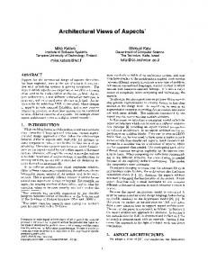
characterizing common knowledge as well. To set up the necessary background for the proof, we now briefly review their fixed-point construction and related characterization of common knowledge. The construction is performed individually by every process i based on its view Vir (m) at a given point (r, m). It defines a sequence of pairs (k` , S` ) consisting of a time and set of processes, for ` ≥ 0. In the construction, F` denotes the set { j : (R, r, k` ) |= DS` ( j is faulty)} of processes known at time k` to be faulty by processes in S` . The sets S` and F` are analogous to, but in general distinct from, to the sets Gi (k) and Bi (k) in C ON C ON. The construction proceeds inductively as follows.

Base: Set k0 = m and S0 = {i}.


39

Step: Set k`+1 = m − (t + 1 − |F` |) and S`+1 = P \ F` . As Moses and Tuttle show, the F` ’s form a nonincreasing sequence of sets of processes. As a result, the S` ’s form a nondecreasing sequence of sets of processes, and the k` ’s form a descending sequence of indices. Since |F` | ≤ t, for some index h we must have that Fh = Fh−1 . When this happens for the first time, the construction reaches ˆ m) and Sˆ = S(r, ˆ m) to a fixed-point because Sh+1 = Sh and kh+1 = kh . We use kˆ = k(r, denote the first values kh and Sh at which a fixed-point is reached. The construction can reach two types of fixed-points. One in which kˆ < 0 (and Sˆ = P), and the other in which kˆ ≥ 0. To accommodate the former case, we define VP (m0 ) = λ for all m0 < 0. (Recall that λ is used to denote the empty view.) We remark that at the fixed point, Fh is the complement of Sh . Since S0 is a singleton and all members of every F` are faulty, the assumption that t ≤ n − 2 guarantees that h ≥ 1 at the fixed point. The final step of the construction is:

Output:

ˆ (We denote this view by Vˆ i [r, m].) The view VSˆ (k).

As shown in [4], process i’s local state Vi (k0 ) at time k0 contains VS` (k` ) for all k` ≥ 0. As a result, process i can compute all of the stages of the construction at time m = k0 based on its local state there. Let r = FIP(ζ, β). When the construction is performed at (r, m), the sets S` and F` depend only on the β component (failures) in r. It follows that the final output Vˆ i [r, m] of the construction depends only on β and on the restriction of ζ ˆ m].3 Figure 3.6 illustrates an example computation of (the inputs) to the nodes of V[r, the fixed-point construction. The fixed-point construction is shown to characterize N-reachability relation (and hence also the common knowledge) in the crash and omission models: Proposition 3.11 (Moses and Tuttle) Let r and r0 be runs of a FIP system R, and assume 3 We

ˆ m] the view Vˆ j [r, m] obtained by the nonfaulty processes j in r, since Vˆ j [r, m] shall denote by V[r,

is the same for all nonfaulty processes j, by Proposition 3.11.


40 r F2 r r r r r r r S r 2 r r

r F=F ˆ 3 r r r r r ˆ 3 r S=S r r r r ˆ 3 k=k

k2

r r r F1 r r r r r r S r 1 r k1

r r r r F0 r r r r i r S0 r r k0 = m

Figure 3.6: An instance of Moses and Tuttle’s fixed-point construction by i at time m. that i is a nonfaulty process in r and j a nonfaulty process in r0 . Then (r0 , m) is Nreachable from (r, m) iff Vˆ j [r0 , m] = Vˆ i [r, m]. In other words, Proposition 3.11 states that the fixed-point construction performed by a nonfaulty process i at (r, m) outputs the same view as the one it outputs for any nonfaulty process at any point in the N-connected component of (r, m). Proposition 3.11 ˆ m] summarizes and uniquely determines the thus implies that, in a precise sense, V[r, set of facts that are common knowledge at any given point (r, m). As a result, we can show that only input events of E that appear in Vˆ are common knowledge among the nonfaulty processes: Corollary 3.12 Let q ∈ ΦE , let P be a

FIP ,

and assume that i is nonfaulty in r. Then

(RP , r, m) |= CN q iff q ∈ E (Vˆ i [r, m]). Proof:

Fix r =

FIP (ζ, β)

∈ R and m ≥ 0, let i be nonfaulty in r, let q ∈ ΦE and let

V = Vˆ i [r, m]. To prove the ‘if’ direction, assume that q ∈ E (V). By Proposition 3.11, V = Vˆ j (r0 , m) for every nonfaulty processor j at a point (r0 , m) that is N-reachable from 0

(r, m). It follows that V is contained in Gr , and q ∈ E (V) implies that (R, r0 , m) |= q. Since this holds for all points N-reachable from (r, m), we have that (R, r, m) |= CN q.


41

For the ‘only if’ direction, assume that q ∈ / E (V). By definition of E (V), it follows that (R, r0 , m) 6|= q for some run r0 = FIP(ζ0 , β0 ) whose execution graph contains V. In particular, ζ and ζ0 agree on the inputs at the nodes of V. Consider the run r00 = FIP(ζ0 , β) with the same failure pattern (β) as in r, and the same external inputs (ζ0 ) as in r0 . The assumption that inputs in R = R(n,t, fm, I ) are independent of failures and of each other ensures that r00 ∈ R. Since q ∈ ΦE it depends only on the external inputs. Since (R, r0 , m) 6|= q, and the fact that r00 shares ζ0 with r0 implies that (R, r00 , m) 6|= q. Recall, that the nodes and edges of the execution graph in V = Vˆ i [r, m] depend only on the failure pattern β. Moreover, since r and r00 share the same failure pattern β, process i is nonfaulty in r00 as it is in r. Since, in addition, ζ0 agrees with ζ on the inputs assigned to ˆ 00 , m] = V = V[r, ˆ m]. Proposition 3.11 implies that (r00 , m) nodes of V, it follows that V[r is N-reachable from (r, m). Hence, from (R, r00 , m) 6|= q we obtain that (R, r, m) 6|= CN q and we are done.

Based on this characterization, we can prove our claim that C ON C ON is optimal: Proof of Theorem 3.10: Fix a run r of FIP. We will abuse notation slightly and denote ˆ m] the runs of both P and C ON C ON with execution graph Gr by the same name r, and V[r, ˆ By Proposition 3.9, the events in M P [m] are common knowledge. By definition by V. i ˆ We will of the core, MiP [m] ⊆ ΦE . Hence, Corollary 3.12 implies that MiP [m] ⊆ E (V). show that Vˆ is contained in VG(c) (c) for c = critri (m). Since MiC [m] = E (VG(c) (c)), this ˆ ⊇ M P [m], from which the claim follows. The case in will imply that MiC [m] ⊇ E (V) i which Vˆ = λ is immediate, since λ is by definition contained in all views, including VG(c) (c). It remains to consider the case in which Vˆ = 6 λ. In this case, let kˆ = kh and Sˆ = Sh be the fixed-point values in the Moses and Tuttle construction performed in the run r. Since Vˆ 6= λ we have that kˆ ≥ 0. Moreover, recall that the construction ends with h ≥ 1 since t ≤ n − 2. Since kh is the first place at which a fixed-point is obtained, we obtain that kh < kh−1 ≤ k0 . Observe that the sets F` in the fixed-point construction contain only faulty processes. Since i ∈ S0 and i is nonfaulty, it follows that i ∈ S`


42

for every ` ≤ h. In particular, i ∈ Sh−1 . By definition of Sh and Fh−1 , we have that Sh = { j : (R, r, kh−1 ) |= ¬DSh−1 ( j is faulty)}. Since i ∈ Sh−1 , we have in particular that (R, r, kh−1 ) |= ¬Ki ( j is faulty), for all j ∈ Sh . It follows that Sh ⊆ Gi (kh−1 − 1), where Gi is the set of good processes according to i in C ON C ON. From kh < kh−1 we have that kh ≤ kh−1 − 1. The perfect recall property of the

FIP

implies that the sets Gi (k)

are monotonically nonincreasing. Thus, Sh ⊆ Gi (kh−1 − 1) ⊆ Gi (kh ). It follows that Bi (kh ) ⊇ Fh , and hence also that bi (kh ) ≥ |Fh |. Since kh = kˆ is the fixed point, we have that kh = m − (t + 1 − |Fh |) and hence m = kh + t + 1 − |Fh |. By definition of C ON C ON, horizoni (kh ) = kh + t + 1 − bi (kh ). Since bi (kh ) ≥ |Fh |, we obtain that horizoni (kh ) ≤ m.

ˆ It follows that VG(c) (c) ⊇ Vˆ and we are By Proposition 3.6(a) we have that critri (m) ≥ k. done.

Extending the core.

So far, the monitored events that we allowed (which we identified

with the propositions in ΦE ) have been facts about the external inputs to the system. This is reasonable because such facts are independent of the protocol used to implement continuous consensus, and such events allow us to monitor information that is relevant in a broad range of applications. It is possible, however, to extend the core and allow it to monitor events that are concerned with the failure pattern as well as the external inputs. In the context of the

FIP

this could actually determine all communications and

all message contents. We say that a proposition p ∈ Φ is objective if its truth depends on the failure pattern and input assignment of the run. Namely, if there is a set Tp of pairs (ζ, β) such that, for every run r0 = FIP(ζ0 , β0 ) and time m0 , we have that (R, r0 , m0 ) |= p exactly if (ζ0 , β0 ) ∈ Tp . In particular, an objective proposition is independent of time. Notice that the propositions in ΦE , which depend on the external input component, ζ, of the run, are by definition objective propositions. Another feature of the new definition is that an objective proposition has the same truth value in runs of different protocols, because Tp is independent of the protocol being followed.


43

We can now define an extended continuous consensus problem, whose specification differs from the original problem only in that the core consists of a set Φ0E ⊆ Φ of objective facts. The proof of Theorem 3.8 shows that the view VGi (c) (c) computed by a nonfaulty process i in the C ON C ON protocol at a point (r, k) is shared among the nonfaulty processes, and hence contained in Vˆ i [r, k]. The proof of Theorem 3.10 shows that VGi (c) (c) contains Vˆ i [r, k]. Thus, the C ON C ON protocol executed at nonfaulty processes ˆ k] at each point (r, k). The information in V[r, ˆ k] can imply that cerin fact computes V[r, tain processes are faulty, and that particular messages were sent successfully in the run while others were not. By Proposition 3.9 all of this information is common knowledge at (r, k). But there may be (objective) facts about the failure pattern that are common knowledge at (r, k) and do not appear explicitly in V[r, k]. For example, there are no explicit failures and/or successful message deliveries in the empty view λ. Nevertheless, if, for example, Vˆ i [r, 3] = λ then among other things the nonfaulty processes did not discover t failures in the first round. This translates into an objective fact q about the run. ˆ k] for the nonfaulty processes And since, as shown in Proposition 3.9, the identity of V[r, is common knowledge, CN q would hold at (r, 3) in this case. In order to obtain an optimum solution for the extended continuous consensus problem, we need to add this type of fact to the core. We do this by replacing the definition of E (V) used in C ON C ON by ˆ k] = V}. E 0 (V, k) , {q ∈ Φ0E : (R, r, k) |= q for all points (r, k) such that V[r, We denote by C ON C ON0 the protocol obtained from C ON C ON by replacing E (λ) by

E 0 (λ, k) and replacing E (VGi (c) (c)) by E 0 (VGi (c) (c), k) on line 5. Since C ON C ON0 comˆ m] at every point (r, m), we obtain an analogous result to Corolputes the view V[r, lary 3.12 for arbitrary objective propositions in Φ0E . An analogous proof to that of Theorem 3.10 can now be shown to yield: Corollary 3.13 C ON C ON0 is an optimum protocol for the extended continuous consensus problem.


3.3

44

Waste and C ON C ON

Waste The concept of waste was defined in [3]. In this section we shall review the definition of waste and extend the term further to define local waste. The task discussed in [3] was obtaining agreement in a crash failure model about the initial configuration of the system. Waste was defined in the context of this analysis. Local waste is a generalization of waste, which helps us analyze when agreement can be reached about any fact in the system (rather than just about time k = 0). Moreover, our definition of local waste will apply to both the crash and the omission models. Recall that according to Theorem 3.2, once it becomes common knowledge that a clean round has occurred, all the facts about the initial configuration become common knowledge. It is easy to show that at time t + 1 it is common knowledge that a clean round has occurred during the first t + 1 rounds, and thus all the facts about the initial configuration are common knowledge. However, if k + j failures are discovered by the end of round k, Dwork and Moses’ analysis in [3] shows that by the end of round t +1− j there must be a clean round. Moreover, it can be shown that by the end of round t + 1 − j it is common knowledge that a clean round has occurred. From the point of view of an adversary trying to delay the agreement as much as possible, this may be considered as a “waste” of j failures. We now formally define the waste of a run, W (r). First, define N (r, k) as the number of faulty processes discovered by time k in r. Next, we define d(r, k) as the difference between N (r, k) and k, and finally we can define the waste, W (r), as the maximal value of d(r, k):

N (r, k) , max{ j : (r, k) |= D(“ j processes have f ailed”)}

(3.6)

d(r, k) , N (r, k) − k

(3.7)


45

W (r) , max d(r, k) k≥0

(3.8)

Note that in this subsection the operators D and C refer to distributed knowledge and common knowledge w.r.t. the set of active processes. The analysis in [3] shows that at the end of round t + 1 −W (r) it is common knowledge that a clean round has occurred in the run. Thus at t + 1 −W (r) all facts about the initial configuration of the nonfaulty processes become common knowledge. The concept is summarized in the following lemma from [3], which is quoted here without proof: Lemma 3.14 Let ϕ be a fact about the initial configuration. Then: (r,t + 1 −W (r)) |= Dϕ iff (r,t + 1 −W (r)) |= Cϕ. Lemma 3.14 implies that at the end of round t + 1 − W (r), any fact known to an active process 4 at time k = 0 becomes common knowledge. An immediate corollary of Lemma 3.14 is the following: Corollary 3.15 Let ϕ be a fact about the initial configuration. If (r, 0) |= DN ϕ then (r,t + 1 −W (r)) |= CN ϕ. Proof:

Assume (r, 0) |= DN ϕ. It is easy to see that also (r,t + 1 − W (r)) |= DN ϕ,

and thus (r,t + 1 − W (r)) |= Dϕ. By Lemma 3.14 we have that (r,t + 1 − W (r)) |= Cϕ, i.e., that ϕ is common knowledge among the active processes, A(r,t + 1 − W (r)). It is straightforward from the definition of common knowledge that any fact which is common knowledge among the active processes, is also common knowledge among any subset of this set. Since N ⊆ A(r,t + 1 −W (r)), we obtain (r,t + 1 −W (r)) |= CN ϕ, and we are done. 4 An

active process w.r.t. time t + 1 −W (r)


46

We refer to the last round, `w in which d(r, k) reaches its maximal value as the round in which the waste was reached, i.e., `w = max{arg max d(r, k)}. An interesting k≥0

property, which is straightforward from the definition of waste, the round following the last time the waste is reached — round `w + 1 — is a clean round.

A Generalized Definition of Waste The concept of waste was defined in the context of the crash model, and was aimed at analyzing when facts about time k = 0 can be agreed upon. Local waste is an extension to the definition of waste, which relates to any time k ≥ 0. In addition, our analysis in this subsection will be relevant to both the crash and the omission models. A key difference between waste and local waste is that waste is a property of the run, W (r), (m)

whereas the local waste, Wi

, is a value which is computed locally with respect to a

specific time m, and a process i. Moreover, two different nonfaulty processes, i and j, (m)

may compute different local wastes w.r.t. a time m, i.e., Wi

(m)

6= W j

. We omit the r

from our definitions, as it is clear from context. We now present three definitions that lead to the notion of local waste:

N (m)

di

(m) i (k) , bi (k) − bi (m)

(k) , N

(m)

Wi

(m) i (k)

− (k − m)

(m)

, max di k≥m

(m)

Notice that for m = 0, the definition of Wi

(k)

(3.9)

(3.10)

(3.11)

bares a strong resemblance to the def-

inition of waste from the previous subsection, with the exception that bi (k) plays the role of N (r, k). This observation is not surprising, since bi (k) in the omission model is analogous to N (r, k) in the crash model. Once again, we define the last round, `lw

3. Solving Continuous Consensus (m)

in which di

47

(k) reaches its maximal value as the round in which the local waste is (m)

reached, or more formally, `lw = max{arg max di k≥m

(k)}. The following lemma captures

the connection between local waste and common knowledge. Lemma 3.16 Let i be a nonfaulty process, let r be a run of (m)

(r , m + (t + 1 − bi (m) −Wi

FIP .

If (r, m) |= DN ϕ, then

)) |= CN ϕ. (m)

Proof: Define κ , m + (t + 1 − bi (m) − Wi

). Since r is a run of a full-information

protocol, let us assume without loss of generality that i is running C ON C ON.5 Thus at m process i computes horizoni (m). Define `lw as the round in which the local waste was (m)

reached. From Equations 3.9- 3.11 we have that Wi

= (bi (`lw ) − bi (m)) − (`lw − m).

At the end of round `lw , process i computes the horizon according to C ON C ON, and we have that:

horizoni (`lw ) = `lw + t + 1 − bi (`lw ) =

(3.12)

= `lw + t + 1 − bi (`lw ) + bi (m) − bi (m) + m − m = = [m + t + 1 − bi (m)] − [(bi (`lw ) − bi (m)) − (`lw − m)] = (m)

= [m + t + 1 − bi (m)] − Wi

,κ

Since horizoni (`lw ) = κ, from Proposition 3.6(a) we have that criti (κ) ≥ `lw . Without loss of generality, assume criti (κ) = `0 ≥ `lw . Thus Mi [κ] = VGi (`0 ) (`0 ). Now since (r, m) |= DN ϕ by the assumption, and since N ⊂ Gi (`0 ), we necessarily have ϕ ∈ VGi (`0 ) (`0 ), and thus ϕ ∈ Mi [κ]. From Proposition 3.9 we have that (r, κ) |= CN ϕ, and we are done. 5 We

require that i will run C ON C ON is order to be able to define horizoni (·), however running C ON -

C ON is not a necessary condition for the correctness of the lemma


48

Lemma 3.16 presents the strong connection between local waste and common knowledge, by showing that facts about time m become common knowledge (t − bi (m)) + 1 − (m)

Wi

rounds after m. For the special case of m = 0, it is interesting to compare our anal-

ysis in this subsection regarding the local waste, to the analysis in [3]. We first present the following lemma, which argues that waste is indeed a special case of local waste. Lemma 3.17 Let i be a nonfaulty process, let R be a system in the crash failure model, i.e., fm = crash, and let r ∈ R be a run of FIP. Moreover, let `w and `lw be the rounds in (0)

which the waste W (r) and the local waste Wi

are reached, respectively. Then:

(i) `w = `lw (0)

(ii) Wi

= W (r)

Proof: For (i), assume by way of contradiction that `w 6= `lw . Notice that since `w is the round in which the waste is reached, round `w + 1 must be clean, which means that no failure is discovered by the active processes. Notice that Gi (`w ) ⊆ A(r, `w ), since Gi (`w ) does not include processes whose faulty behavior was discovered by i in round `w +1. Notice also that Gi (`w ) ⊇ A(r, `w ), since if there is a process j ∈ A(r, `w )\Gi (`w ), then j’s faulty behavior must be discovered by the nonfaulty process i in round `w + 1, which not possible since `w + 1 is a clean round. Thus we have that Gi (`w ) = A(r, `w ). Notice that using a similar argument Gi (`lw ) = A(r, `lw ) also holds. Since N (r, `w ) is computed according to the knowledge of the set A(r, `w ), and bi (`w + 1) is based on the knowledge of Gi (`w ), it follows that bi (`w ) = N (r, `w ). We thus have that d(r, `w ) = (0)

(0)

di (`w ). Similarly, we also have bi (`lw ) = N (r, `lw ), and thus d(r, `lw ) = di (`lw ). (0)

(0)

Now assume `w > `lw , and thus d(r, `w ) ≥ d(r, `lw ). It follows that di (`w ) ≥ di (`lw ), which contradicts the fact that `lw is the round in which the local waste is reached. (0)

(0)

Assume, on the other hand that `w < `lw , and thus di (`w ) ≤ di (`lw ), which means that d(r, `w ) ≥ d(r, `lw ), contradicting the fact that `w is the round in which the waste is reached. Thus `w = `lw .


49 (0)

For (ii), since `w = `lw , and we have shown that also d(r, `w ) = di (`w ), by the (0)

definition of Wi

(0)

and W (r) it follows that Wi

= W (r), and we are done.

Lemma 3.17 shows that our analysis of the local waste is a direct enhancement of Dwork and Moses’ analysis of waste in the crash model. The result in Lemma 3.16 both extends the previous analysis to the omission failure model, and generalizes the discussion from agreeing about the initial configuration to agreeing on facts about any later time m. By using the results of C ON C ON from the previous sections, we were able to prove Lemma 3.16, which is a direct generalization of Lemma 3.15. Following the proof of Lemma 3.16, it is interesting to observe that κ = horizoni (m)− (m)

Wi

, and thus an immediate corollary is:

Corollary 3.18 Let i be a nonfaulty process, let r be a run of (m)

about time m. If (r, m) |= Dϕ, then (r , horizoni (m) −Wi

FIP ,

and let ϕ be a fact

)) |= Cϕ.

Our proof of Lemma 3.16 made use of C ON C ON, however, Corollary 3.18 presents an even stronger connection between local waste and C ON C ON. Indeed, we defined horizoni (m) as process i’s upper bound on the destination of m, and showed that in

fact i’s estimation for m’s destination may be improved compared to horizoni (m). By (m)

Corollary 3.18 we realize that this improvement is precisely Wi

.

The following lemma will complete the picture regarding the connection between local waste and C ON C ON. Lemma 3.19 Let i be a nonfaulty process, let m ≥ 0, and let r be a run of FIP. Further(m)

more, let `lw be the round in which the local waste, Wi (m)

(a) `lw = criti (horizoni (m) −Wi

)

(m)

(b) desti (m) = horizoni (m) −Wi

is reached. Then:

3. Solving Continuous Consensus Proof:

50 (m)

Define κ , horizoni (m) − Wi

. The proof of Lemma 3.16 showed us that

criti (κ) ≥ m. In order to show that `lw = criti (κ), let us assume by way of contradiction that `lw < criti (κ), i.e., that criti (κ) = `0 > `lw . Thus by our analysis of C ON C ON, it is easy to see that horizoni (`0 ) = κ. By the proof of Lemma 3.16, we have that also horizoni (`lw ) = κ, and thus:

horizoni (`lw ) = horizoni (`0 )

(3.13)

`lw + t + 1 − bi (`lw ) = `0 + t + 1 − bi (`0 ) bi (`lw ) − `lw = bi (`0 ) − `lw

Now also notice that:

(m)

di

(`0 ) = N

(m) 0 0 0 0 i (` ) − (` − m) = (bi (` ) − bi (m)) − (` − m)

(3.14)

= bi (`0 ) − `0 + m − bi (m) = bi (`lw ) − `lw + m − bi (m) (m)

= (bi (`lw ) − bi (m)) − (`lw − m) = di

(m)

And thus we have di

(m)

(`lw ) = di

(`lw )

(`0 ), which contradicts our definition of `lw , as

the latest round at which the waste is reached, and we are done with part (a). Recall that desti (m) = κ exactly if criti (κ) ≥ m, and criti (κ − 1) < m. The proof of Lemma 3.16 showed us that criti (κ) ≥ m. In order to prove that criti (κ − 1) < m, let us assume by way of contradiction that criti (κ − 1) , m0 ≥ m. Thus horizoni (m0 ) = κ − 1, and recall that `lw = criti (κ).


51

κ − 1 = horizoni (m0 ) = horizoni (`lw ) − 1

(3.15)

m0 + t + 1 − bi (m0 ) = `lw + t + 1 − bi (`lw ) − 1 bi (m0 ) − m0 = bi (`lw ) − `lw + 1 (m)

And if we observe di (m)

di

(m0 ), we find that:

(m0 ) = (bi (m0 ) − bi (m)) − (m0 − m)

(3.16)

= bi (m0 ) − m0 + m − bi (m) = bi (`lw ) − `lw + 1 + m − bi (m) (m)

= (bi (`lw ) − bi (m)) − (`lw − m) + 1 = di (m)

And we obtain that di

(m)

(m0 ) = di

(`lw ) + 1

(`lw ) + 1, which contradicts the assumption that (m)

`lw is the round in which the value of di

(·) is maximal, and we are done with (b) as

well. By Lemma 3.19(b) we have that the i’s horizon and i’s local waste at m uniquely de(m)

termine m’s destination, which is precisely horizoni (m)−Wi (m)

shows that at horizoni (m) − Wi

. Moreover, Lemma 3.19(a)

all facts about the first `lw rounds become common

knowledge.

3.4

Clean Rounds Revisited

In our description of clean rounds in Section 3.1, we said that up to this work clean rounds were discussed in the context of the crash model. After having presented C ON C ON, we extend the definition of clean rounds to the omission model. We say that a


52

round k is clean if bi (k − 1) = bi (k) for all nonfaulty processes i. Thus, it is not the discovery of a failure in a round that makes it dirty; rather, a round is dirty if, for some process z, it is the first round in which z’s failure is reported by a process that is trusted by some nonfaulty process. Intuitively, it is straightforward from the definition of horizon that our computation of horizoni (m) = m + (t + 1) − bi (m) guarantees that there exists at least one round k, such

that m < k ≤ horizoni (m), in which bi (k −1) = bi (k). This fact does not guarantee a clean round, however, the following lemma implies that indeed a clean round is guaranteed to occur in this interval. Lemma 3.20 Let i be a nonfaulty process. Then for all k ≥ 0 if criti (k) = m 6= −1 then m + 1 is a clean round. Proof: Assume by way of contradiction that for some nonfaulty j we have b j (m) 6= b j (m + 1). By definition of B j , we have that b j is a nondecreasing function of m, and thus b j (m) < b j (m + 1). Since both i and j are nonfaulty, we have by Theorem 3.8 that criti (k) = crit j (k) = m. It follows that horizon j (m) = k. Since b j (m) < b j (m + 1), it follows by the definition of horizon that horizon j (m) ≥ horizon j (m + 1). By Proposition 3.6(a) crit j (k) ≥ m + 1, which contradicts the fact that crit j (k) = m, and we are done. Thus the round following a critical time must be a clean round. In fact, this observation is not surprising following Section 3.3, since by Lemma 3.19 and by the fact (m)

that horizoni (m) = k we have that Wi

(m)

= 0, and thus m is the round in which Wi (m)

reached. It is immediate from the definition of Wi

is

that the next round, m + 1, must be

clean. Another interesting property of clean rounds in our context is presented below. Lemma 3.21 Let m + 1 be a clean round. Then Bi (m) ∪ Gi (m) = P for every nonfaulty process i.

3. Solving Continuous Consensus Proof:

53

Assume by way of contradiction that for some nonfaulty i there exists an m

and a process j such that m + 1 is a clean round and j 6∈ Gi (m) ∪ Bi (m). Since i is nonfaulty, we have i ∈ Gi (m + 1), and since i knows about j’s faulty behavior at time m + 1, we have j ∈ Bi (m + 1), while we assumed j 6∈ Bi (m). Thus it must be the case that bi (m + 1) > bi (m), which is in contradiction to the assumption that m + 1 is a clean round. Notice that Lemmas 3.20 and 3.21 imply that if m is a critical time of some k, then Bi (m) ∪ Gi (m). Intuitively, Moses and Tuttle’s fixed-point construction (Figure 3.6) proposed a similar claim, however their definitions of the sets of faulty and nonfaulty processes, the sets F and S are a bit different than our definitions of good and bad processes. Finally, we conclude this section by presenting the following lemma: Lemma 3.22 Let ϕ be a fact about the first k − 1 rounds, let i be a nonfaulty process in r and assume that S = Gi (k − 1). If (r, k − 1) |= DS (ϕ) and round k of r is clean, then (r, k) |= EN ϕ. Proof: Assume that round k is clean, and that (r, k − 1) |= DS (ϕ). We shall prove that (r, k) |= EN ϕ by showing that for all nonfaulty processes, j, we have that (r, k) |= K j ϕ. Assume that j is nonfaulty. We claim that Bi (k − 1) = B j (k − 1). Assume by way of contradiction that Bi (k − 1) 6= B j (k − 1). Without loss of generality, assume that there exists a process z ∈ Bi (k − 1) \ B j (k − 1). Thus, at time k process i knows about z’s failure. Since i is nonfaulty, we have that i ∈ G j (k), and thus z ∈ B j (k). It follows that B j (k − 1) 6= B j (k), which contradicts the assumption that k is a clean round. Thus we have that Bi (k − 1) = B j (k − 1). Since round k is clean, Lemma 3.21 implies that we also have S = Gi (k − 1) = G j (k − 1). It follows that (r, k − 1) |= DS (ϕ). Notice that by the definition of G j (k − 1), all messages from processes in G j (k − 1) are delivered to j successfully in round k, and since we assume a FIP, we must have that (r, k) |= K j ϕ, and we are done.


54

One of the key results by Dwork and Moses [3], which is presented in Theorem 3.1, is that following a clean round every fact that was previously distributed knowledge, becomes known to all the nonfaulty processes. By Lemma 3.22, we see that the same result holds in the omission model, in the context of clean rounds as presented in this section. It follows that our new definition of clean rounds plays essentially the same role in the omission model as the original definition of clean rounds played in the crash model; after a clean round all nonfaulty processes share a consistent view of the system.

3.5

A Run of C ON C ON

In this section we discuss some interesting properties of the C ON C ON protocol, of the horizon, and of the sets of good and bad processes. We discuss these properties by

presenting an example of a run, r of C ON C ON. In our example n = 16, t = 6, and we assume that processes i and j are nonfaulty.

The horizon Revisited Intuitively, we described horizoni (k) as process i’s estimation of when facts about time k will join the core. Figure 3.7 gives further intuition about the horizon, by showing horizoni and horizon j as a function of k for two nonfaulty processes, i and j in r. Let us

point out some observations about r, which are illustrated in Figure 3.7. These observations follow from the properties of the horizon which were described in Section 3.1. • No processes are initially known to be faulty, i.e., bi (0) = 0, and thus horizoni (0) = t + 1 = 7. • The horizon increases by at most one in every round. • Horizons at different processes are not necessarily the same, e.g., horizoni (9) = 14, while horizon j (9) = 15 (however, recall that the correct processes’ horizons are identical at a critical time).


55

• The graph shows the function f (k) = k as a reference, since in a way it can be thought of as an “asymptote” of the horizon. If the system reaches a point (r, k) at which bi (k) = t, i.e., all faulty processes have been discovered, then for all ` > k we will have horizoni (`) = ` + 1. Indeed, in our example we can see that at any time ` > 16, we have horizoni (`) = ` + 1.

20

horizon(k)

15

horizoni(k) horizonj(k) f(k)=k

10

5

0 0

5

10

15

20

k

Figure 3.7: The Horizon vs. k in a run r.

Critical Times Revisited In Figure 3.8 we can see a graph of the critical time, criti (k) as a function of k for r. Notice the following observations: • There are times which are not critical times, e.g., 12 is not the critical time of any k. • If horizoni (k) 6= horizon j (k) then k cannot be a critical time. This follows from Theorem 3.6, since if k = criti (`) of some time `, then it must be so for all nonfaulty processes i. In our example, horizoni (12) 6= horizon j (12), and indeed 12 is not a critical time.


56

• If criti (k) = m, then we can check in Figure 3.7 and see that indeed horizoni (m) = k. For example, Figure 3.8 shows that criti (10) = 4, and in Figure 3.7 we can see that horizoni (4) = 10. • Much like the graph of the horizon, we show f (k) = k as a reference, and similarly, it can be thought of as an “asymptote” for criti (k), with criti (`) = `−1 when bi = t.

20 crit(k) f(k)=k 15

crit(k)

10

5

0 0

5

10

15

20

-5 k

Figure 3.8: Critical time vs. k in a run r.

Good and Bad Processes Revisited Our subtle definitions of the good and bad process are the basis of the horizon computation, and are thus a key notion in C ON C ON. As discussed in Section 3.1, our definition of Gi (k) uses i’s knowledge at time k + 1, enabling i to receive information about round k from all processes in Gi (k), and thus i’s computation of Bi (k) is based on the knowledge of all the good processes Gi (k). The following properties are straightforward from the definitions of G and B, and can be seen quite vividly in Figure 3.9: • Notice that Gi (k) and Bi (k) are distinct sets, i.e., Gi (k) ∩ Bi (k) = 0/ for all k.


57

• Bi is a monotonously nondecreasing set, i.e., Bi (k) ⊆ Bi (k + 1), and Gi is a monotonously nonincreasing set, i.e., Gi (k) ⊇ Gi (k + 1). • Another interesting property of B and G, which is a corollary of Lemma 3.21, is that if m is a critical time of some k, i.e., m = criti (k), then we have Bi (m) ∪ Gi (m) = P. For example, recall from the previous subsection that criti (10) = 4, and indeed we can see in Figure 3.9 that Bi (4) ∪ Gi (4) = P. • By Lemma 3.20 it follows that round 5 must be clean, and indeed we can see that bi (4) = bi (5).

Figure 3.9: Gi (k) and Bi (k) in r.

Local Waste and Destination Figure 3.10 shows desti (k) and horizoni (k) as a function of k. The following observations may be seen from the graph: • It is possible for several points, m, m0 to have the same destination. For example, desti (9) = desti (10) = 14. Recall that for this reason the destination is not defined as crit−1 i .


58

• Process i’s horizon at m is an estimation of desti (m). As we can see in Figure 3.10, indeed desti (m) and horizoni (m) are equivalent most of the time. By Lemma 3.19 we have that the connection between the horizon and the destination is desti (m) = (m)

horizoni (m) −Wi

, and thus the destination is different than the horizon at times

(m)

> 0. In our particular example, the only such time m is m = 12.

m in which Wi 20

15

horizoni(k) desti(k) f(k)=k

10

5

0 0

5

10

15

20

k

Figure 3.10: desti (k) and horizoni (k) in r. (m)

Figure 3.11 illustrates the computation of the local waste, Wi 3.11(a), presents N • Since N

(0) i (k),

(0) i (k)

and the second, 3.11(b) shows N

(12) (k). i

. The first graph,

Observe that:

= bi (k), 3.11(a) in fact shows the number of bad processes as a

function of k. (0)

• Notice that in our example Wi

= 0, since no failures are discovered “fast enough”

after time 0. On the other hand, as we can see in 3.11(b) since bi (k) increases by (12)

2 in round 13, we have that Wi

=1 (m)

• In both graphs we present k − m as a reference. Recall that di

(m)

(k − m), and that the waste is reached when the difference, di

(k) = N

(m) i (k) −

(k), is maximal. In

3. Solving Continuous Consensus (m)

the graphs, di when N

(m) i (k)

(k) is positive precisely when N

59 (m) i (k) is over the k −m line.

Thus

reaches its highest point over the k − m line, the waste is reached.

In our example for m = 12, the only time at which N k = 13, which is when the waste is reached.

(12) (k) i

is over the line is at


60

20

N(k)

15

N(k) k-m

10

5

0 0

5

10

15

20

k

(a) N

(0) i (k)

vs. k for m = 0.

N(k)

10

N(k) k-m

5

0 0

5

10

15

k

(b) N

(12) (k) i

vs. k for m = 12.

Figure 3.11: Local Waste

20

Chapter 4 Uniform Continuous Consensus 4.1

The UCC Problem

The continuous consensus problem specifies constraints only on the cores of nonfaulty processes, guaranteeing nothing about faulty ones. Observe, however, that failures in our models are not considered malicious—there is no lying and faulty behavior is closely related to crashing or communication malfunction. It is thus natural to consider a stronger version of the problem, which we call uniform continuous consensus (UCC). The specification of UCC is similar to that of CC (see Section 3.1), except that Accuracy and Consistency are required to hold for arbitrary processes and not just for nonfaulty ones. Completeness, however, is still restricted to events that are known to nonfaulty processes: If an event e ∈ E is known to a nonfaulty process j at any point, then e ∈ Mi [k] must hold (for all processes i, of course) at some time k. One can expect a solution to UCC to be similar in spirit to C ON C ON, because the failures we consider, both in the crash and the (sending) omission models, only affect the ability of a process to send messages, so that even faulty processes receive all incoming messages. In this chapter we consider how the C ON C ON protocol can be modified to obtain U NI C ON C ON, an optimal protocol for UCC. As shown in [2, 5], simultaneously consistent behavior by all participants is closely related to (standard) common knowledge, that is, the traditional notion equivalent to an infinite conjunction of “everyone knows” (while in the previous chapter our analysis

4. Uniform Continuous Consensus

62

referred to common knowledge among the nonfaulty processes). Common knowledge among all processes (see Section 2.6) and UCC are related in the same way as CN and continuous consensus are, and a result analogous to Proposition 3.9 holds. Neiger and Tuttle [10] show that in our settings (crash and omission failure models) the two notions of common knowledge coincide: Theorem 4.1 (Neiger and Tuttle) R |= (Cϕ ≡ CN ϕ) for every formula ϕ and

FIP

sys-

tem R. Intuitively, the claim of Theorem 4.1 can be explained by the fact that failures in these models affect only the ability of a process to send messages; even faulty processes receive all incoming messages. A natural question in light of Theorem 4.1 is whether C ON C ON itself solves the UCC problem. Unfortunately, it does not. The problem with using C ON C ON is that a faulty process x might know of failures at time k but not tell the nonfaulty processes. If x ∈ Gx (k), then these failures will be counted in bx (k) and will therefore play a role in determining horizonx (k), but if x is silent from round k + 1 on, for example, then these failures will not affect the calculations of other processes. An inconsistency between x’s core and those of the nonfaulty processes will arise as a consequence.

A protocol for UCC We now present a variant of C ON C ON, called U NI C ON C ON, that solves the UCC problem. The U NI C ON C ON protocol is based on the following intuition. Whether or not a process x is faulty, it is still guaranteed in our models to receive all messages that are sent to it. Moreover, if g ∈ Gx (k), then no nonfaulty process has discovered that g is faulty by time k − 1. The information available to g at time k − 2 has thus been transmitted to the (truly) nonfaulty processes in round k − 1, and they are guaranteed to relay it to x (and to all other processes) in round k. Hence, a possibly faulty process x can simulate in round k what a nonfaulty process g would compute two rounds earlier. As a result, it is possible to design a uniform protocol that mimics the behavior of C ON C ON as long


63

as the distance to the horizon is three rounds or more. Special care needs to be taken when the distance to the horizon becomes two rounds or one. In this section we use i, j, x, z, g ∈ P to denote processes in our system, such that i and j are nonfaulty processes, x and z are potentially faulty processes, and g is a good process.1 The U NI C ON C ON protocol is given in Figure 4.1. We distinguish the values of Latesti , criti and Mi computed in C ON C ON from the corresponding values computed in U NI C ON C ON by adding the superscript u to instances of the latter. On line 2 of the protocol, the process x chooses an arbitrary member g of Gx (k − 1) whose computation in round k − 2 of C ON C ON process x will simulate in round k.2 Notice that horizong (k − 3) is available to x in round k because x’s local state has a copy of Vg (k − 2) (since otherwise g ∈ / Gx (k − 1)). Lines 4, 5 and 6 of U NI C ON C ON play the same role as lines 3, 4 and 5 of C ON C ON respectively. On lines 3 and 4 of U NI C ON C ON process x simulates what a nonfaulty process would have computed two rounds earlier. Line 5 computes the critical time, distinguishing three distinct cases: there are special tests for whether the critical time is one or two rounds back; when neither is the case, the process uses the critical time obtained by simulating the critical round that a seemingly nonfaulty process would compute in C ON C ON. Finally, line 6 computes the core in much the same way as in C ON C ON. The correctness claim for U NI C ON C ON is summarized by the following theorem: Theorem 4.2 Fix a run r in a FIP system R. Let i be a nonfaulty process in r, let x be an arbitrary process, and let k ≥ 1. Then Mxu [k] = Mi [k]. The proof of Theorem 4.2 as well as intermediate lemmas used in its proof are presented in Appendix A.2. An immediate corollary of Theorems 4.1 and 4.2 is Corollary 4.3 U NI C ON C ON is an optimum protocol for Uniform Continuous Consensus. 1 Good 2A

here stands simply for the fact that g ∈ Gx (k) for some process x at a certain time k of interest. process x can choose itself as g as long as x ∈ Gx (k − 1), so that x does not know that it is faulty.


U NI C ON C ON(x) 0

1 2 3 4

5

6

Latestxu [`] ← −1 for all ` ≥ 1 for every round k ≥ 1 do send local state and receive messages according to FIP g ← arbitrary member of Gx (k − 1) if k ≥ 3 then compute Gg (k − 3), Bg (k − 3) and horizong (k − 3) x simulates g’s behavior in C O N C O N : Latestxu [horizong (k − 3)] ← k − 3 endif   if horizonx (k − 1) = k k − 1 u c ← k−2 if horizong (k − 2) = k ∧ horizonx (k − 1) 6= k   u Latestx [k] otherwise   if cu = −1 E (λ) Mxu [k] ← E (VGx (k−1) (k − 1)) if cu = k − 1 ≥ 0   E (VGg (cu ) (cu )) otherwise endfor

Figure 4.1: Process x’s computation in U NI C ON C ON.

64

Chapter 5 Conclusion In the present study we have presented and analyzed the continuous consensus (CC) problem, which generalizes simultaneously consistent action in fault-prone synchronous systems. Using a knowledge-based approach, a solution to the CC problem called C ON C ON was presented, as well as its uniform variant, U NI C ON C ON. These protocols are both simple and optimal. Continuous consensus is closely related to common knowledge. Moreover, the optimal solution to the CC problem is equivalent to computing all the facts that are common knowledge. The definition of the CC problem sheds a new light on the study of simultaneously consistent actions, and allows for a simpler and more intuitive analysis.

5.1

Summary of Results

Continuous Consensus and C ON C ON.

A continuous consensus service requires each

process i to maintain at every time k an up-to-date core Mi [k] of information about the past, so that the cores at all correct processes are guaranteed to be identical. A solution to the CC problem in the crash and omission failure models called C ON C ON was presented. A striking aspect of the solution is its simplicity: At every round, each process updates a single value based on a straightforward computation. Moreover, while the solution is stated in the context of the full-information protocol, it can be implemented in a more efficient manner.

5. Conclusion

66

Optimality and Connection to Common Knowledge.

Continuous consensus is shown

to be closely related to the problem of computing what is common knowledge at any given point. It is shown that the contents of the core Mi [k] of any CC protocol is common knowledge among the nonfaulty processes at time k. Moreover, it is shown that the core computed in C ON C ON contains precisely all the facts that are common knowledge at time k, which the derives optimality of C ON C ON: the core produced by C ON C ON is the largest possible core at any given time. Moreover, the cores of all correct protocols for continuous consensus are subsets of C ON C ON’s core.

Uniform Continuous Consensus.

The uniform variant of the continuous consensus

(UCC) problem requires that all processes, both faulty and nonfaulty, will maintain the same core at all times. Our solution to UCC in the crash and omission models, called U NI C ON C ON, enables a potentially faulty process x to compute in every round k the same core as a nonfaulty process i would produce in C ON C ON, i.e., Mi [k] = Mxu [k]. Process x performs this computation by simulating what a nonfaulty process i would have computed according to C ON C ON. Interestingly, the solution to UCC does not incur any degradation in the information contained in the core of shared information. UCC is related to common knowledge among all processes in the same way that CC is related to common knowledge among the nonfaulty processes. The optimality of U NI C ON C ON follows from Mi [k] = Mxu [k], and from the equivalence in [10]. Clean Rounds.

This work bridges a gap between the analysis of common knowledge

with crash failures in [3] and that for omission failures in [4]. In the case of crash failures, clean rounds are rounds in which no new failures are discovered. However, prior to this work no analogous definition of clean rounds was found in the context of the omission model. The C ON C ON and U NI C ON C ON protocols presented in this work, do, however, suggest a natural generalization of clean rounds to the omission model. We define round k to be clean in this case if bi (k − 1) = bi (k − 2) holds for every nonfaulty process i. We show that if criti (m) 6= −1 then the identity of criti (m),

5. Conclusion

67

as well as the fact that criti (m) + 1 is a clean round, become common knowledge at time m. Moreover, it is shown that a clean round enables all “good” processes to send their messages successfully, allowing the nonfaulty processes to have a consistent view of the system at the end of this round. This key property of clean rounds plays a very similar role in [3] and in the analysis in the present work.

Waste and Local Waste. The term local waste is defined as a direct generalization of the term waste which was defined in [3]. Waste was defined in [3] in the context of the crash model, as a key tool in the analysis of the question when facts about the initial state of the system became common knowledge. Local waste extends this work, and allows for the analysis of the time at which facts about time m become common knowledge. Furthermore, using the analysis of C ON C ON, we show that the properties of waste and local waste in the crash model apply to the omission model as well.

“Good” and “Bad” Processes. Our algorithms shed an interesting light on the distinction between evidence supplied by processes that are known to be faulty and ones that are not. Recall that failures in the models we considered are benign. No process ever deviates from the protocol by sending incorrect messages. Thus, every piece of information obtained from a process can be trusted. Nevertheless, the computation of the horizon by process i in round k, and thus ultimately the times at which common knowledge is obtained, depends only on the set of bad processes, Bi (k − 1). Thus, despite the fact that information from faulty processes is correct, this central computation considers only failures reported by the good processes, i.e., the potentially nonfaulty processes. This distinction seems an essential aspect of the evolution of common knowledge over time in these models.

5. Conclusion

5.2

68

Future Work

Our analysis has hitherto been restricted to the crash and sending omission models. However, the continuous consensus problem is amenable to study and analysis in harsher failure models as well. An extension to the current work [11] (work in progress) considers the CC problem in the generalized omission and the authenticated Byzantine failure models. In the generalized model a faulty process may either omit to send messages or fail to receive them, and thus a message failure does not uniquely identify a faulty process. In the authenticated Byzantine model processes may lie, possibly without ever being discovered as liars. Thus, in both these models it is not possible to define good or bad processes solely based on the message loss in the system, as we did in Chapter 3, which makes the analysis more subtle. Despite these challenges, it is possible to prove an analogous result to Proposition 3.9 for these more complex failure models, i.e., to show that the core, Mi [k], is common knowledge at time k. However, finding a solution to the CC problem which coincides with all the events that are common knowledge (as we did in Chapter 3 for the simpler models) may prove problematic in these models. For example, testing for common knowledge in the generalized omission model was shown in [4] to be an NP-hard computation. Thus, an optimum solution for CC in this model is NP-hard as well. Furthermore, in the Byzantine model we may expect an optimum solution to be even more computationally complex. When we go beyond sending omissions, it is worthwhile to seek tractable solutions to the CC problem that are not necessarily optimal. The authenticated Byzantine model [12] assumes that although faulty processes may be “liars”, they cannot alter any relayed information. This assumption is enforced by using an authentication scheme: all messages sent in the system are authenticated by unforgeable signatures. In the full-information protocol in this model, in every round each process sends a signed message encoding all the information it knows. More specifically, a process i signs and relays every piece of information it receives. The nature of the model enables us to monitor events e of the form “process i claims that p” for some

5. Conclusion

69

process i and proposition p ∈ ΦE . Once i creates a signed message containing e, no other process can forge it. A protocol called ACC (short for authenticated continuous consensus) solves the CC problem in the authenticated Byzantine model, under the assumption that n > 2t. The protocol is fairly simple: When process i receives a message containing an event e signed by a sequence of t + 1 distinct processes, it inserts e into its core. Intuitively, the fact that t + 1 different processes have signed and relayed e before it reached process i guarantees that at least one of the signing processes is nonfaulty. This nonfaulty process will have forwarded the message to all nonfaulty processes, which, in turn, are able to sign and forward it. This guarantees that all nonfaulty processes simultaneously receive a message regarding e with t + 1 signatures. A variant of the ACC protocol is ACC D (short for ACC with d signatures), in which we assume n > t, rather than n > 2t. In ACC D, if process i receives at time k a message containing d signatures by distinct processes about an event e for some d ≤ t + 1, it inserts e into Mi [`]. The time ` = k + t + 1 − d bares some resemblance to the idea of the horizon in Chapter 3. Roughly, it is the time at which e with t + 1 signatures would be delivered to all processes if there were at least t + 1 nonfaulty processes in the system. It can be shown that if a nonfaulty process receives at time k a message bearing d signatures regarding an event e, then at time ` = k + t + 1 − d, the event e will simultaneously appear in the core of all nonfaulty processes. In a sense this protocol is early stopping compared to ACC, since it requires i to process the event e at time k, but e does not require any further attention by i in later rounds. The generalized omission model, in which processes may fail by either omitting to send messages, or failing to receive them, is more complex than the sending omission model, and yet simpler than the authenticated Byzantine model. A solution to the CC problem in this model may be reached by either of the solutions we have seen for the authenticated Byzantine model. However, some measures may be taken to improve any of these protocols, by estimating the number and the identity of the faulty processes in the run according to the omitted messages. This task is, of course, not as simple as in

5. Conclusion

70

the sending omission model, since for example, the fact that process z failed to send a message to process x may imply that either of these processes is faulty. Information about failures in this model can be extracted by keeping track of a conflict graph among processes based on the omitted messages. For example, if a process z has conflicts with more than t others, then it must be faulty. (The minimal vertex covers of the conflict graph yield more detailed information about failures — see, e.g., [4]). Clearly, different information about conflicts is known to different processes at any given time. A key observation is that if we monitor information about conflicts in the core, then it is possible to use information about failures simultaneously and consistently by the different processes. Once the core contains information determining that a process is faulty, this process can be ignored, and the rest can act as if the bound t on the number of failures is reduced by 1. This allows the nonfaulty processes to consistently ”shift gears” as a result of failures appearing in the core. The continuous consensus problem in the harsher failure models has a rich mathematical and promises to provide exciting challenges and insights. [13]

Bibliography [1] T. Mizrahi and Y. Moses, “Continuous consensus via common knowledge,” in Theoretical Aspects of Rationality and Knowledge: Proc. Tenth Conference, pp. 236– 252, 2005. [2] J. Y. Halpern and Y. Moses, “Knowledge and common knowledge in a distributed environment,” Journal of the ACM, vol. 37, no. 3, pp. 549–587, 1990. [3] C. Dwork and Y. Moses, “Knowledge and common knowledge in a Byzantine environment: crash failures,” Information and Computation, vol. 88, no. 2, pp. 156– 186, 1990. [4] Y. Moses and M. R. Tuttle, “Programming simultaneous actions using common knowledge,” Algorithmica, vol. 3, pp. 121–169, 1988. [5] R. Fagin, J. Y. Halpern, Y. Moses, and M. Y. Vardi, Reasoning about Knowledge. Cambridge, Mass.: MIT Press, 1995. [6] P. A. Bernstein, V. Hadzilacos, and N. Goodman, Concurrency Control and Recovery in Database Systems. Addison-Wesley, 1987. [7] L. Lamport, “The part-time parliament,” ACM Trans. on Computer Systems, vol. 16, no. 2, pp. 133–169, 1998. [8] B. A. Coan, D. Dolev, C. Dwork, and L. J. Stockmeyer, “The distributed firing squad problem.,” SIAM J. Comput., vol. 18, no. 5, pp. 990–1012, 1989.

Bibliography

72

[9] B. Coan, “A communication-efficient canonical form for fault-tolerant distributed protocols,” in Proc. 5th ACM Symp. on Principles of Distributed Computing, pp. 63–72, 1986. [10] G. Neiger and M. R. Tuttle, “Common knowledge and consistent simultaneous coordination,” Distributed Computing, vol. 6, no. 3, pp. 181–192, 1993. [11] T. Mizrahi and Y. Moses, “Byzantine continuous consensus,” work in progress, 2006. [12] M. Pease, R. Shostak, and L. Lamport, “Reaching agreement in the presence of faults,” Journal of the ACM, vol. 27, no. 2, pp. 228–234, 1980. [13] A. Bar-Noy, D. Dolev, C. Dwork, and H. R. Strong, “Shifting gears: Changing algorithms on the fly to expedite Byzantine agreement,” vol. 97, pp. 205–233, Apr. 1992.

Appendix A Detailed Proofs A.1

Optimality of C ON C ON Revisited

In Theorem 3.10 we showed that MiP [m] ⊆ MiC [m] holds for a FIP P. In Lemma A.2 we shall show that the same argument holds for an arbitrary protocol. Intuitively, since a full information protocol requires that all processes send all of the information available to them in every round, one would expect this protocol to give each process as much information about events in the system as any protocol could. Thus we expect that the core of a FIP will include at least as much information as that of any other protocol given the exact same environment. We start by quoting the following lemma from [4], which serves us in our proof. Lemma A.1 (Moses and Tuttle) Let ϕ ∈ ΦE , let r be a run of a full-information-protocol P, and let r0 be a run of an arbitrary protocol P , with the exact same execution graph as 0

r, i.e., Gr = Gr . If (RP , r0 , m) |= CN ϕ then (RP , r, m) |= CN ϕ. The following lemma is a corollary of Theorem 3.10, which refers to an arbitrary protocol, P , rather than a FIP protocol. Lemma A.2 Let r0 be a run of an arbitrary protocol P that solves continuous consensus. Then MiP [m] ⊆ MiC [m] for all m.

A. Detailed Proofs Proof: Define a run r of a

74 FIP

0

P such that Gr = Gr . We have to show that for any

primitive fact ϕ, if ϕ ∈ MiP [m], then ϕ ∈ MiC [m]. Assume ϕ ∈ MiP [m]. By Proposition 3.9 we have that the contents of MiP [m] is common knowledge, and thus in particular we have that (r0 , m) |= Cϕ. Then by Lemma A.1 we have that also (r, m) |= Cϕ, which implies that ϕ appears in Vˆ i [r, m]. The proof of Theorem 3.10 showed us that Vˆ i [r, m] ⊆ MiC [m] for every full-information-protocol P, i.e., that all the primitive facts that are common knowledge in r appear in the core, and thus we have ϕ ∈ MiC [m], and we are done.

A.2

Correctness proofs for U NI C ON C ON

In this section we prove Theorem 4.2. The first part of the proof is broken down into a number of claims. In the technical development below, keep in mind that the value of every horizon j (m) is a function of the

FIP

execution and the values of j and m, but not

of the consensus protocol being followed (whether C ON C ON or UniConCon). Lemma A.3 For all x ∈ P, m ≥ 0 and g, g0 ∈ Gx (m + 2), if horizong (m) 6= horizong0 (m), then horizong (m + 1) ≤ min horizoni (m). i∈{g,g0 }

Proof: Since horizong (m) 6= horizong0 (m), we have that either horizong (m) < horizong0 (m) or horizong (m) > horizong0 (m). We consider each case separately. First assume that horizong (m) < horizong0 (m). From the definition of horizon we have that bg (m) >

bg0 (m). It follows from the definitions of Bg (m) and Bg0 (m) that there exists a process z ∈ Gg (m) such that z ∈ / Gg0 (m). Since g, g0 ∈ Gx (m + 2), process g receives a message from g0 in round m + 2, since otherwise g would tell x in round m + 3 that g0 has failed to send a message, and we would have g0 6∈ Gx (m + 2). It follows that g learns of z’s failure from g0 in round m + 2, so z ∈ Bg (m + 1). It follows that at the end of round m + 2 we

A. Detailed Proofs

75

have that bg (m + 1) ≥ bg (m) + 1, and we obtain horizong (m + 1) ≤ horizong (m). Since bg (m) > bg0 (m), and since bg (m) is a nondecreasing function of m, we also have that bg (m + 1) ≥ bg0 (m) + 1, so horizong (m + 1) ≤ horizong0 (m). Now assume that horizong (m) > horizong0 (m). Again, from the definition of horizon, we have that bg (m) < bg0 (m). It follows from the definitions of Bg (m) and Bg0 (m) / Gg (m). Once again, since g, g0 ∈ that there exists a process z ∈ Gg0 (m) such that z ∈ Gx (m + 2), in particular g receives a message from g0 in all rounds up to m + 2, and thus g0 ∈ Gg (m + 1). Since Bg (m + 1) is based on the distributed knowledge of processes in Gg (m + 1) at time m + 1, in particular Bg (m + 1) includes all processes known by g0 at time m + 1 to be bad. Thus we have Bg0 (m) ⊆ Bg (m + 1). Since g ∈ Gx (m + 2), it must be the case that g ∈ Gg (m + 1), since otherwise x would learn of g being faulty in round m + 3. It follows that z’s failure is distributed knowledge at time m + 1 among the processes in Gg (m + 1), and thus by the definition of Bg (m + 1), we have that z ∈ Bg (m + 1). Since Bg0 (m) ⊆ Bg (m + 1) and z ∈ Bg (m + 1), it follows that bg (m + 1) ≥ bg0 (m) + 1, and thus horizong (m + 1) ≤ horizong0 (m). Since horizong0 (m) < horizong (m) by the assumption, we have horizong (m + 1) ≤ horizong (m), and we are done. The next two lemmas provide the formal justification for the choice of critical time in the first two cases of line 5 of the U NI C ON C ON protocol, where critux is not chosen according to the value of Latestxu [k]. The first captures the fact that once the horizon is one round away for at least one process, all t faulty processes are known to the nonfaulty processes, and the identity of the faulty processes becomes common knowledge. Lemma A.4 If r is a run, x, z ∈ P, and k ≥ 1, then: (a) if horizonx (k − 1) = k then Gz (k − 1) = Gx (k − 1); (b) horizonx (k − 1) = k iff horizonz (k − 1) = k.

A. Detailed Proofs

76

Proof: By definition of horizon, we have that horizonx (k −1) = k +t −bx (k −1). Hence, if horizonx (k − 1) = k then bx (k − 1) = t. Let Gx = Gx (k − 1) and Bx = Bx (k − 1). By the definition of Bx (k − 1) and the fact that t is an upper bound on the number of faulty processes, it follows that (R, r, k − 1) |= DGx ( the set of faulty processes is Bx ) and (R, r, k − 1) |= DGx ( the set of nonfaulty processes is Gx ). Every set Gz (m) is guaranteed to contain all nonfaulty processes in r. Since Gx = Gx (k − 1) is the set of nonfaulty processes, it follows that Gz (k − 1) ⊇ Gx (k − 1) = Gx . As a result, the two facts above are distributed knowledge among the processes in Gz (k − 1) / we conclude that Bz (k − 1) = Bx (k − 1) and as well. Since Gz (k − 1) ∩ Bz (k − 1) = 0, Gz (k − 1) = Gx (k − 1). The latter yields part (a) of the claim. By the former, we have that bz (k − 1) = t and so horizonz (k − 1) = k. This establishes the only-if direction of the claim in part (b). Switching the roles of x and z in the proof yields the other direction of (b) and we are done. Lemma A.5 If r is a run, i, x and g are processes such that i is nonfaulty in r, and g ∈ Gx (k − 1), k ≥ 1, and horizonx (k − 1) 6= k, then: (a) if horizong (k − 2) = k then Gg (k − 2) = Gi (k − 2); (b) horizong (k − 2) = k iff horizoni (k − 2) = k. Proof of A.5(a): Since i is nonfaulty, we have that i, g ∈ Gx (k −1), and thus the round k messages of both g and i are received by x. Assume, by way of contradiction, that Gg (k − 2) 6= Gi (k − 2). Thus, there are two distinct cases: (1) Gg (k − 2) \ Gi (k − 2) 6= 0/ :

Let z ∈ Gg (k − 2) \ Gi (k − 2). By the definition of

Gg (k − 2), since z ∈ Gg (k − 2), we have that z ∈ / Bg (k − 2). Recall that Bx (k − 1) is

A. Detailed Proofs

77

computed according to the distributed knowledge of processes in Gx (k − 1). Since i, g ∈ Gx (k − 1), we have that Bx (k − 1) includes all processes known to either i or g at time k − 1 to be bad. Thus Bg (k − 2) ⊆ Bx (k − 1) and z ∈ Bx (k − 1). Now since z∈ / Bg (k − 2), we have that Bx (k − 1) = Bg (k − 2) ∪ {z}. Since horizong (k − 2) = k by the assumption, we have horizong (k − 2) = (k − 2) + t + 1 − bg (k − 2) = k, and thus bg (k − 2) = t − 1. Hence we have that bx (k − 1) = bg (k − 2) + 1 = (t − 1) + 1 = t. It now follows that horizonx (k − 1) = (k − 1) + t + 1 − bx (k − 1) = k, contradicting the assumption that horizonx (k − 1) 6= k. (2) Gi (k − 2) \ Gg (k − 2) 6= 0/ :

Let z ∈ Gi (k − 2) \ Gg (k − 2). In this case, too, we

distinguish two distinct cases. If z ∈ / Bg (k − 2), then this case is very similar to (1), and thus by using essentially the same argument, again we reach a contradiction. On the other hand, assume z ∈ Bg (k − 2). Thus z’s faulty behavior is distributed knowledge among the processes in Gg (k − 2), and thus at time k − 2 some process z0 ∈ Gg (k − 2) knows that z is faulty. It is easy to see that z0 fails to send its messages to i in round k − 1, since had it successfully sent to i, process i would have known that z is faulty, causing z ∈ / Gi (k − 2). Since z0 fails to send to i in round k − 1, we have z0 ∈ / Gi (k − 2). Since z0 ∈ Gg (k − 2), by the definition of Gg (k − 2) we have that z0 ∈ / Bg (k − 2). Again, as in (1), Since i, g ∈ Gx (k − 1), we have that Bx (k − 1) includes all processes known to either i or g at time k − 1 to be bad. Thus Bx (k − 1) = Bg (k − 2) ∪ {z0 }, and again we have bx (k − 1) = t, which implies that horizonx (k − 1) = (k − 1) + t + 1 − bx (k − 1) = k, contradicting the assumption that horizonx (k − 1) 6= k. Proof of A.5(b):

For part (b), our proof consists of two parts:

(1) We first assume that horizong (k −2) = k and show that horizoni (k −2) = horizong (k − 2). Assume, by way of contradiction, that horizoni (k − 2) 6= horizong (k − 2), i.e., either horizoni (k − 2) < horizong (k − 2) or horizoni (k − 2) > horizong (k − 2). We shall handle each of the two cases separately.

A. Detailed Proofs horizoni (k − 2) < horizong (k − 2):

78 By our assumption for part (b) we have that

horizong (k − 2) = k, and thus if horizoni (k − 2) < horizong (k − 2), then it must

be the case that horizoni (k − 2) ≤ k − 1. By definition of horizon, and since the number of bad processes is bounded by t, we have horizoni (k − 2) = (k − 2) + t + 1 − bi (k − 2) ≥ (k − 2) + t + 1 − t = k − 2. Since both horizoni (k − 2) ≤ k − 1 and horizoni (k − 2) ≥ k − 1, we have that horizoni (k − 2) = k − 1. Since by definition horizoni (k − 2) = (k − 2) + t + 1 − bi (k − 2), we have that bi (k − 2) = t. From the definition of Bi (k − 2), we have that Bi (k − 2) ⊆ Bi (k − 1), and thus bi (k − 2) ≤ bi (k − 1). It follows that bi (k − 1) = t, and thus horizoni (k − 1) = k. By Lemma A.4(b) we obtain that horizonx (k − 1) = k, which contradicts the assumption that horizonx (k − 1) 6= k.

horizoni (k − 2) > horizong (k − 2):

By the definition of horizon, it follows that

bi (k − 2) < bg (k − 2). It then follows that Bi (k − 2) 6= Bg (k − 2), and thus from the definitions of Bi (k − 2) and Bg (k − 2) we have that Gi (k − 2) 6= Gg (k − 2), although horizong (k − 2) = k by the assumption, which contradicts part (a). We have shown that if horizong (k − 2) = k then horizoni (k − 2) = k. (2) For the second half of the proof, we assume that horizoni (k − 2) = k, and we have to show that horizoni (k − 2) = horizong (k − 2). Again, we assume by way of contradiction that horizoni (k − 2) 6= horizong (k − 2), and distinguish the two possible cases.

horizoni (k − 2) > horizong (k − 2):

The proof is similar to the first half of (1).

horizoni (k −2) < horizong (k −2):

By the assumption we have that horizoni (k −

2) = k, and thus it is easy to see from the definition of horizon we have that bi (k − 2) = t − 1. Since horizoni (k − 2) < horizong (k − 2), by the definition of horizon we have that bi (k − 2) > bg (k − 2). Hence there exists a process z ∈ Bi (k − 2) \

A. Detailed Proofs

79

Bg (k − 2). Thus z’s faulty behavior is distributed knowledge among the processes in Gi (k − 2), and thus at time k − 2 some process z0 ∈ Gi (k − 2) knows that z is faulty. Since z ∈ / Bg (k − 2), it follows that z0 ∈ / Gg (k − 2), since otherwise the faulty behavior of z would be distributed knowledge among Gg (k − 2), causing z ∈ Bg (k − 2). Since z0 ∈ Gi (k − 2), by the definition of Gi (k − 2) we have that z0 ∈ / Bi (k − 2). Since i, g ∈ Gx (k − 1), we have that Bx (k − 1) includes all processes known to either i or g at time k − 1 to be bad. As we have seen, z0 ∈ / Bi (k − 2), and thus Bx (k − 1) = Bg (k − 2) ∪ {z0 }. It follows that bx (k − 1) = bi (k − 2) + 1 = (t −1)+1 = t, which implies that horizonx (k −1) = (k −1)+t +1−bx (k −1) = k, contradicting the assumption that horizonx (k − 1) 6= k. We are now ready to prove that the critical time critux (k) chosen in U NI C ON C ON by an arbitrary process x is the same as the corresponding time criti (k) that is chosen in the same FIP execution by a nonfaulty process in the C ON C ON protocol. Lemma A.6 Let i be a nonfaulty process in r, let x be an arbitrary process, let k ≥ 1, and let g ∈ Gx (k − 1). If horizonx (k − 1) 6= k and horizong (k − 2) 6= k, then critux (k) = criti (k). Proof: Let m = criti (k). By lines 3 and 4 of C ON C ON, it follows that k = horizoni (m). By Lemma A.5(b), horizong0 (k − 2) = k iff horizoni (k − 2) = k for all g0 ∈ Gx (k − 1). Hence, since horizonx (k − 1) 6= k and horizong (k − 2) 6= k, we have that critux (k) is assigned Latestxu [k] in the third case of line 5 in U NI C ON C ON. By line 5 of the protocol, we thus have that critux (k) ≤ k − 3. Also notice that horizoni (k − 1) 6= k and horizoni (k − 2) 6= k by Lemmas A.4(b) and A.5(b) respectively, and thus criti (k) ≤ k − 3.

We claim that critux (k) = criti (k). Assume, by way of contradiction, that critux (k) 6= criti (k). We consider two distinct cases. • First, suppose that critux (k) < criti (k). We claim that horizong (m) = horizoni (m) for all g ∈ Gx (m + 2). Assume, again by way of contradiction that horizong (m) 6=

A. Detailed Proofs

80

horizoni (m). Then we have by Lemma A.3 that horizoni (m + 1) ≤ horizoni (m).

By assumption, m = criti (k), and in particular horizoni (m) = k. It follows that horizoni (m + 1) ≤ k. By Proposition 3.6(a) we have that criti (k) ≥ m + 1, which

contradicts the assumption that m , criti (k). We have proved that horizong (m) = k for all g ∈ Gx (m + 2), and thus in round m + 3 when process x executes line 4 of U NI C ON C ON, it assigns Latestxu [k] the value m. Notice that Latestxu [k] may be updated again on line 4 of the protocol at a later round ` > m + 3, but it can then be assigned only values ` − 3 > m. It follows that Latestxu [k] ≥ m. Recall that we have shown that criti (k) ≤ k − 3, which implies that k ≥ m + 3. Since Latestxu [k] ≥ m holds at time m + 3 and at any later time, it follows that critux (k) ≥ m = criti (k), contradicting the assumption that critux (k) < criti (k). • Now suppose that critux (k) > criti (k). Let critux (k) = mu > −1. Thus by lines 4 and 5 of U NI C ON C ON for some g ∈ Gx (mu + 2) we have that horizong (mu ) = k. We shall prove that horizong (mu ) = horizoni (mu ). Assume by way of contradiction that horizong (mu ) 6= horizoni (mu ) then by Lemma A.3 we have horizoni (mu +1) ≤ horizong (mu ) = k. Thus by Proposition 3.6(a), we have that critux (k) ≥ mu + 1,

which is in contradiction to the fact that critux (k) = mu . We have shown that horizong (mu ) = horizoni (mu ), i.e., that horizoni (mu ) = k. By Proposition 3.6(b)

we obtain criti (k) ≥ mu = critux (k), contradicting the assumption that critux (k) > criti (k), and we are done. We can now finally prove the correctness of U NI C ON C ON: Proof of Theorem 4.2:

We first argue that process x has access to all of the data

necessary to carry out the actions specified in every line of U NI C ON C ON. Since knowledge is defined with respect to the fixed system of runs of the

FIP ,

process x can de-

termine the identity of the members of Gx (k − 1) at time k. Hence, x can perform the choice of g ∈ Gx (k − 1) on line 2. Moreover, observe that for every g0 ∈ Gx (k − 1), at

A. Detailed Proofs

81

time k process x has a copy of Vg0 (k0 ) for all k0 ≤ k − 1. It follows that x can compute horizong (k − 3) used on line 4, as well as horizong (k − 2) used in the middle case of

line 5. Finally, it can compute E (VGx (k−1) (k − 1)) and E (VGg (cu ) (cu )) when cu < k − 1, and thus is able to perform the commands on line 6. It remains to show that critux (k) = criti (k) and that Gi (c) = Gg (c) for all g ∈ Gx (k − 1). From line 6 in U NI C ON C ON and line 5 in C ON C ON, it will then follow that Mxu [k] = Mi [k]. Notice that line 5 of U NI C ON C ON assigns one of three values to critux (k). Thus in our proof we handle the three possible assignments on line 5 as three distinct cases. Theses cases are indeed distinct since each of the first two cases in the assignment on line 5 implies that the value of critux (k) is k − 1 or k − 2 respectively, while the third case on line 5 assigns Latestxu [k] to critux (k). Notice that Latestxu [k] is last updated in some round m ≤ k on line 4 of U NI C ON C ON, and thus the value assigned to Latestxu [k] was m−3. Thus Latestxu [k] = m−3 ≤ k −3, and thus in the third case of line 5 we necessarily have critux (k) ≤ k − 3.

critux (k) = k − 1 : By line 5 of U NI C ON C ON we have that horizonx (k − 1) = k. Thus, by Lemma A.4(b) we also have that horizoni (k − 1) = k, and hence criti (k) = critux (k) = k − 1. By Lemma A.4(a) we have that Gz (k − 1) = Gi (k − 1) for all z ∈ P, and in particular Gx (k − 1) = Gi (k − 1). It follows that Mxu [k] = Mi [k].

critux (k) = k − 2 : Since critux (k) = k − 2, by line 5 of U NI C ON C ON we have that horizong (k − 2) = k for some g ∈ Gx (k − 1), and also that horizonx (k − 1) 6= k. By

Lemma A.5(b) we have that horizoni (k − 2) = k, and by Lemma A.4(b) we have that horizoni (k − 1) 6= k. Thus, in round k − 1 on line 3 of C ON C ON process i assigns k − 2

to Latesti [k], and Latesti [k] is not updated in round k. It follows that criti (k) = k − 2. By Lemma A.5(a) we have that Gg (k − 2) = Gi (k − 2), and we again obtain that Mxu [k] = Mi [k].

A. Detailed Proofs

82

critux (k) < k − 2: This case applies only if k ≥ 2. By Line 5 of U NI C ON C ON, in this case we have that critux (k) = Latestxu [k]. Moreover, by Lemma A.6 we have that critux (k) = criti (k). Let c , critux (k) = criti (k). It remains to show that Gi (c) = Gg (c). Set g ∈ Gx (k − 1). Assume by way of contradiction that Gi (c) 6= Gg (c). First we claim that bi (c + 1) > bi (c). Notice that in round c + 2 both i and g receive each other’s messages, since g ∈ Gx (c + 2), and i is nonfaulty. If there exists a p ∈ Gi (c) such that p ∈ / Gg (c), then process i learns of p’s failure from g in round c + 2, and moreover, p ∈ Bi (c + 1), and thus bi (c + 1) > bi (c). On the other hand, if there exists a p ∈ / Gi (c) such that p ∈ Gg (c), then it must be the case that i learns of p’s faulty behavior in round c + 1, and thus p ∈ / Bi (c). However, p ∈ Bi (c + 1), and thus again bi (c + 1) > bi (c). Thus, in all cases bi (c + 1) > bi (c), and by the definition of horizon we have that horizoni (c + 1) ≤ horizoni (c). Thus, by the definition of c, we have that horizoni (c + 1) ≤ k. Now, from

Proposition 3.6(a) we obtain that criti (k) ≥ c + 1, i.e., that c ≥ c + 1, which contradicts our assumption, and we are done with the third case. d

Maintaining Simultaneously Consistent Views of a ... - CiteSeerX

Maintaining Simultaneously Consistent Views of a ... - CiteSeerX

Suggest Documents

Maintaining Simultaneously Consistent Views of a ... - Google Sites

Maintaining Views Incrementally - CiteSeerX

Maintaining Consistent Transactional States ... - People.csail.mit.edu

Maintaining Recursive Views of Regions and ... - CIS @ UPenn

Views to a Kill - CiteSeerX

Views to a Kill - CiteSeerX

Maintaining a Jointly Constructed Student Model - CiteSeerX

Conversion of heat and light simultaneously using a ... - CiteSeerX

Maintaining Multiple Motion Model Hypotheses Over Many Views to ...

Efficiently Maintaining Distributed Model-Based Views ... - Google Sites

Maintaining Multiple Motion Model Hypotheses Over Many Views to ...

Consistent Equivalence Relations: a Set-Theoretical ... - CiteSeerX

SIREN: a memory-conserving, snapshot-consistent ... - CiteSeerX

A Thermodynamically Consistent Damage Model for ... - CiteSeerX

SIREN: a memory-conserving, snapshot-consistent ... - CiteSeerX

Simultaneously Learning and Optimizing using Controlled ... - CiteSeerX

Estimating multiple option Greeks simultaneously using ... - CiteSeerX

Architectural Views of Aspects - CiteSeerX

Simultaneously measured current, luminosity, and electric ... - CiteSeerX

Central pattern generating neurons simultaneously ... - CiteSeerX

SyncViews: Toward Consistent User Views in Cloud-based File ...

Unifying Views of UML - CiteSeerX

Simultaneously Viewing Monoscopic and Stereoscopic ... - CiteSeerX

Efficiency Evaluation of a Photovoltaic System Simultaneously ...