Majority support for progressive income taxation: The importance of corner preferences. Philippe De Donder∗ Universite de Toulouse (IDEI and GREMAQ) and Jean Hindriks∗∗ CORE, Universite Catholique de Louvain and Queen Mary, University of London 07 January 2002
Abstract:This paper studies voting over quadratic taxation when income is fixed and taxation non distortionary. We first show that, if a Condorcet winner (a tax function preferred by a majority to any other feasible tax function) exists, it involves maximum progressivity. We then give necessary and sufficient conditions on the income distribution for a Condorcet winner to exist, and show numerically that these conditions are satisfied for a large class of distribution functions. The existence of a Condorcet winner is due to the fact that the feasible set is closed (because of incentive compatibility constraints) and that individuals have corner preferences over this set. JEL classification: D72 Keywords: Majority Voting; Income Taxation; Tax Progressivity.
∗ Manufacture
des Tabacs, 21 allée de Brienne, 31000 Toulouse, France, Email:
[email protected] ∗∗
CORE, Voie du Roman Pays 34, B-1348 Louvain-la-Neuve, Belgium. Tel. (32 10)-478163, Email:
[email protected]
1
Introduction
Why is it that many democracies have adopted progressive income taxes (Snyder and Kramer(1988), Cukierman and Meltzer(1991))? It is difficult to provide a normative justification to such a feature, since the optimal taxation literature has proved inconclusive on the shape of the tax function (see Myles(2000) for a recent account)1 . Moreover, a positive explanation based on the self-interest of citizens/voters seems more in line with the reality of the choice of tax schemes. Unfortunately, the political economy approach suffers from a problem of equilibrium existence due to the multidimensionality of the voting problem. To allow voters (or their representatives) to choose between both progressive and regressive tax schemes, the set of feasible tax schedules must be at least bidimensional. But we know since Plott(1967) that it is highly unlikely to find a Condorcet winner (an option preferred by a majority to any other feasible option) in multidimensional settings. The reason for the inexistence of a Condorcet winner can be explained directly in the context of the vote over multidimensional taxes with fixed income (i.e. non distortionary taxation). Marhuenda and Ortuno-Ortin(1995) have shown that for income distributions where median income is below mean income, any concave tax scheme receives less popular support than any convex tax scheme provided that the latter treats the poorest agent no worse than the former. The majority in favor of progressivity (i.e. convex tax function) is composed of low income individuals who thereby shift the burden of taxation towards high incomes. On the other hand, Hindriks(2001) has shown in the context of quadratic tax functions that for any convex tax function there is a concave one that is supported by a majority of voters. This majority is composed of both low and high income people who favor the regressivity because it shifts the burden of tax towards middle 1
On the other hand, Young (1990) has shown that when the planner’s objective is to choose a “fair” tax schedule, the equal sacrifice requirement implies progressive taxation.
1
income voters. Putting together Marhuenda and Ortuno-Ortin(1995) and Hindriks(2001) results in the cyclicity of the majority voting rule, resulting in the absence of a Condorcet winner. Political economy papers studying taxation adopt various strategies to face this inexistence problem. Early papers (Romer (1975), Roberts (1977)) reduce the policy space to linear tax schedules and obtain a Condorcet winner involving average progressivity. Berliant and Gouveia (1994) introduce uncertainty over the income distribution and then use the ex-ante budget balance requirement to reduce the policy space so that a Condorcet winner exists. Snyder and Kramer(1988) assume that candidates cannot credibly commit to implement something different from their most-preferred policy and thus restrict the policy space to the policies that are ideal for some voter. Roemer (1999) is not interested in Condorcet winners but uses a different solution concept (called the Party Unanimity Nash Equilibrium) based on the need to reach an intra-party consensus among ’opportunists’ whose only objective is to win the elections, and ’militants’ who care only about the policy chosen by their party. This paper wishes to stress that the usual proofs of the inexistence of a Condorcet winner (such as in Plott(1967)) crucially depend on the candidate policy to be in the interior of the policy set. If this set is closed, and if voters have corner preferences, it is much easier to obtain a Condorcet winner on the boundary of the feasible set, since directions favored by a majority of voters may be infeasible2 . The rest of the paper applies this idea to the political choice of taxation. More precisely, we present in Section 2 the model studied by Roemer(1999) where income is fixed and taxation quadratic. We show in Section 3 that incentive constraints result in the policy set to be closed, and that individuals 2
Both Marhuenda and Ortuno-Ortin(1995) and Hindriks(2001) assume that it is possible to construct a (respectively) more and less progressive tax schedule, i.e. they also assume that the tax schedule under consideration belongs to the interior of the feasible set.
2
all have corner solutions over this set. We show that, if a Condorcet winner exists, it involves maximum progressivity (Proposition 2) and we give necessary and sufficient conditions on the income distribution for a Condorcet winner to exist (Proposition 3). We then use numerical illustrations to show the plausibility of these conditions, and find that they are satisfied for a large class of income distributions. Section 4 concludes by stressing the generality, but also the weaknesses, of our approach.
2
The Model
We consider an economy populated by a large number of individuals who differ only in their (fixed) income level. Each individual is characterized by her income, y ∈ [0, 1]. The distribution of income in the population is described by a strictly increasing cumulative distribution function F on [0, 1], so that F (y) is the fraction of the population with pre-tax income less or equal to y. The average pre-tax income is Z 1 y= ydF (y)
(1)
0
and the median pre-tax income is 1 ym = F −1 ( ). 2
(2)
We assume throughout that ym ≤ y , i.e. we restrict ourselves to positively skewed income distributions as typically observed in real world. For every individual with pre-tax income y, the after-tax income is
x(y, t) = y − t(y)
(3)
where t(y) is a continuous tax function t : R+ → R. Note that we allow for negative taxes. Definition 1. A tax function is feasible if it satisfies the following conditions, 3
t(y) ≤ y
for all y ∈ R+
for all y ∈ R+ 0 ≤ t0 (y) ≤ 1 Z 1 t(y)dF (y) = 0
(4) (5) (6)
0
Condition (4) says that tax liabilities cannot exceed taxable income. Condition (5) implies that both tax liabilities and after-tax income are nondecreasing functions of pre-tax income.3 The budget balance condition (6) means that income taxation is purely redistributive (i.e., zero revenue requirement). Our primary objective is to understand when progressive taxation emerges as a voting outcome. We adopt the following definition of progressivity.4 Definition 2: A tax schedule is (marginally) progressive if and only if t(y) is a convex function (i.e. marginal tax rates are monotonically increasing). The set of potential tax schedules is infinitely dimensional. To limit the voting problem over tax policies to a manageable number of dimensions we shall thereafter restrict attention to the quadratic income tax function. t(y) = −c + by + ay 2
(7)
where c ≥ 0 is the uniform lump-sum transfer, b is the flat tax parameter (with 0 ≤ b ≤ 1) and a is the progressivity tax parameter, with a > 0 indicating a (marginally) progressive income tax and a < 0 representing a 3
This condition is usually derived instead of assumed in the optimal income tax literature with endogenous labor supply. Non-decreasing tax function is not required in Roemer (1999). 4 Since we allow for negative taxes our definition of progressivity (marginal progressivity) does not necessarily correspond to the more usual definition of progressivity in terms of increasing average tax rates (average progressivity) which gives a better indication of the level of redistribution. But since the objective of this paper is to understand the prevalence of (weakly) convex tax function rather than the level of redistribution, the concept of marginal progressivity seems more appropriate
4
(marginally) regressive one. It is readily checked that the feasibility conditions (4) and (5) impose the following lower and upper bounds on the progressivity parameter:
−b 2
≤a≤
1−b 2
. Essentially, the upper bound on
progressivity ensures that the marginal tax rate is less than one at the top (and thus everywhere) and the lower bound on regressivity guarantees that marginal tax rate is positive at the top (and thus everywhere). Combining (6) and (7) yields c = by + ay 2
(8)
R
y 2 dF (y). Hence, tax policies are bidimensional. Let the set of © ª 1−b feasible tax policies be T = (a, b) ∈ [ −b 2 , 2 ] × [0, 1] . Plugging (7) and (8)
where y2 =
into (3) the after-tax income (consumption) of an individual with pre-tax income y resulting from a tax policy (a, b) ∈ T is given by x = y + (1 − b)(y − y) − a(y2 − y 2 ).
(9)
In this simple setting, the distribution of income is independent of the tax policy and each individual only cares about his after-tax income as given by (9). We now turn to the voting problem over (non-linear) tax policies (a, b) ∈ T . A majority (or Condorcet) winning tax policy is a pair (a, b) that is preferred by a majority of individuals to any other feasible pair (a0 , b0 ) ∈ T . In the next section, we show that in general a majority winning policy exists and that it involves progressive taxes. The intuition behind the existence result is that individuals vote for tax policies that are on the boundary of the feasible set.
3
Voting equilibrium
We first look at the preferences of the voters in the (a, b) space5 . An individual with pre-tax income y is indifferent about a tax change dt = (da, db) if 5
This description is borrowed from Roemer(1999).
5
dx = (y − y)db + (y 2 − y 2 )da = 0
(10)
Indifference curves can be represented by straight lines in the policy space with slopes y − y2 db (y) = −[ 2 ] ≡ −ϕ(y). da y−y
(11)
It appears (see Figure 1 below) that this function is increasing in y, with √ ϕ(0) = ϕ( yy2 ) = yy2 , ϕ( y2 ) = 0, ϕ(1) < 2 and asymptotic values ϕ(y− ) = +∞ and ϕ(y+ ) = −∞. There exists also a unique y1 such that ϕ(y1 ) = 2. p It is given by y1 = 1 − (1 − y)2 + σ 2 with σ 2 > 0 the variance of the √ income distribution. Note that y − σ < y1 < y < y 2 < y + σ. The directions of utility increase are
da > 0, db > 0 for 0 ≤ y ≤ y p da > 0, db < 0 for y < y ≤ y 2 p da < 0, db < 0 for y 2 < y ≤ 1
6
(12)
ϕ(y)
6
(0, 2)
³ ´ 0, yy¯¯2
y1
√ y¯2
y¯
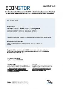
Figure 1 (Roemer, 1999): Slope of indifference curves in the (a, b)-space Using these observations about the indifference curves we can derive by a simple geometric argument the preferred policy of each individual. To do this it is convenient to break the income range into four separate intervals: √ √ Y1 = [0, y1 ]; Y2 = (y1 , y]; Y3 = (y, y 2 ]; Y4 = ( y2 , 1]. The set of feasible tax policies is illustrated in Figure 2 by the parallelogram Γ = OABC with
7
-
1
y
the indifference curves of a member of each income group Y1 to Y4 and the directions of utility increase. 6b
H HH HH C H1H B s 7 ¶ H TH T ¶ H T T HH T T H (y ∈ Y1 ) T T T T T T T T T T T T T T T T T T (y ∈ Y2 ) T T : » T T LL »» T T L T (y ∈ Y4 ) Q T L ´ ´ Q T TL ´ ¶ Q T ´ TL / ¶ Q T ´ Q 0 TL A T´´- a Ts Q Q ´ L ´ 1/2 1/2 0 QQ L ´ Q L ´ Z ~ Z L (y ∈ Y3 ) L Figure 2: Feasible set and indifference curves
It follows from the construction of the income groups that (1) for all y ∈ Y1 : the indifference curve is negatively sloped and flatter than AB since 0 < ϕ(y) < 2; and utility increases in the North-East, since y < y. Hence, B is the preferred policy of each member of this group (note that for the limit case y = y1 , the indifference curve is parallel to AB and this individual is actually indifferent between all policies on the boundary AB ). (2) for all y ∈ Y2 : the indifference curve is negatively sloped and steeper than AB since 2 < ϕ(y) < +∞; and utility increases in the North-East, since y < y. Hence, A is the preferred policy of this group (note that for
8
the limit case y = y, the indifference curve is vertical and utility increases √ in the East direction, since y < y2 . Hence A is also the preferred policy). (3) for all y ∈ Y3 : the indifference curve is positively sloped since ϕ(y) ≤ √ 0; and utility increases in the South-East, since y < y ≤ y2 . Hence, the preferred policy of this income group is A (note that for the limit case √ y = y 2 , the indifference curve is horizontal and this individual is actually indifferent between all policies on the boundary 0A ). (4) for all y ∈ Y4 : the indifference curve is negatively sloped and flatter than OC since ϕ(1) < 2; and utility increases in the South-West, since √ y 2 < y. Hence, O is the preferred policy of this income group. This leads to the following lemma. Lemma 1: The preferred policy (a, b) is (i) B = (0, 1) for all 0 ≤ y ≤ y1 ; (confiscation) √ (ii) A = ( 12 , 0) for all y1 < y ≤ y 2 ; (maximum progressivity); √ (iii) O = (0, 0) for all y2 < y ≤ 1 (no taxation). We are now in a position to show that a majority winner in general exists in this environment with no incentive effects. The following proposition is a direct consequence of Lemma 1. Proposition 1: Given y1 = 1 −
p (1 − y)2 + σ 2 < y,
(a) if ym ≤ y1 then the tax policy B = (0, 1) is a majority winner. √ (b) if ym > y1 and F ( y 2 )−F (y1 ) ≥ 1/2, then the tax policy A = ( 12 , 0) is a majority winner. If a majority of individuals belong to the low income group (Y1 ), the voting outcome will be the confiscation policy, whereas if a majority belong to the middle income group (Y2 + Y3 ) the voting outcome will be maximum progressivity. The latter case is not surprising as progressivity enables the middle class to minimize its own tax burden at the expenses of the rich and the poor. We now turn to the less straightforward case in which neither the low income group nor the middle-income group form a majority on their own. 9
We show that in this case the only potential Condorcet winner is the most progressive policy. √ Proposition 2: Assume that F ( y 2 ) − F (y1 ) < 1/2 with y1 < ym √ < y 2 . Then either the most progressive policy A = ( 12 , 0) is a majority winner or there is no majority winner. √ y2 prefer the policy (a + ε, b) √ < y < y 2 , they form a majority
Proof. Note first that all individuals y < to the policy (a, b), with ε > 0. Since ym
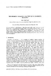
and any policy not belonging to the segment AB [see Figure 2] is defeated by this majority. Second, all individuals y > y1 prefer policy A = ( 12 , 0) to any other policy belonging to the segment AB. Since y1 < ym , they form a majority, and policy A is the only potential majority winning policy.¥ Proposition 2 says that if the median voter prefers the most progressive policy A, then any majority winner must consist of that policy even though this is not optimal for a majority of individuals. Of course there remains the possibility that a majority winner fails to exist. This is the case if there exists a feasible deviation from policy A that is desirable for a majority of individuals. The following proposition gives a necessary and sufficient condition for such deviation not to exist and thus for policy A to be the majority winner. Proposition 3: Under the condition of Proposition 2, a necessary and sufficient condition for policy A to be the majority winner is that F (y2 (ϕ)) √ (ϕ−2y)2 +4σ2 ϕ −F (y1 (ϕ)) ≥ 1/2 ∀ϕ ∈ (ϕ(0), ϕ(1)) where yi (ϕ) = 2 ± . 2 Proof. To prove that policy A is a majority winner under the conditions stated in proposition 3, we must show that there exists no feasible deviation from that point that could be supported by a majority coalition. Let us db be the denote any tax change from A = ( 12 , 0) by da and db and let dτ = − da
direction of tax change. It is obvious from Figure 3 that the only feasible tax changes are 0 ≤ dτ ≤ 2 with da < 0. Comparing all the possible directions of tax change dτ with the properties of individual indifference curves as 10
given in (11)-(12) we can determine the set of individuals favorable to any tax change. First note that all changes of the type dτ ∈ [0, ϕ(0)] can be disregarded since dτ ≤ ϕ(0) implies that all those with y ≤ ym are against the reform. Similarly all changes of the type dτ ∈ [ϕ(1), 2] can also be disregarded since dτ ≥ ϕ(1) implies that all those with y ≥ ym are against the reform. Hence the only candidates to defeat policy A are tax changes of the type dτ ∈ Λ = (ϕ(0), ϕ(1)). Moreover each individual whose indifference curve is such that ϕ(y) = dτ is indifferent. It will prove useful to identify any tax change (dτ ) by the slope of the indifference curve of the indifferent agent (say, ϕ). From (11), it appears that the function ϕ(y) is not one-to one in the relevant range Λ and that for each ϕ ∈ Λ one can associate the √ (ϕ−2y)2 +4σ2 ϕ following two income levels: y1 (ϕ), y2 (ϕ) = 2 ± . It can be 2 shown that y1 (ϕ) is increasing and concave with domain Λ and range [0, y1 ) whereas y2 (ϕ) is increasing and convex with domain Λ and range [ yy2 , 1]. For each reform ϕ ∈ Λ, the set of individuals favoring the reform is given by all the poor with income y < y1 (ϕ) and all the rich with income y > y2 (ϕ). Policy A is thus a majority winner iff for each ϕ ∈ (ϕ(0), ϕ(1)), F (y2 (ϕ)) −F (y1 (ϕ)) ≥ 1/2, (with y1 (ϕ) < y1
y1 (ϕ)) who do not find the increase in b big enough to compensate for the lower a and some rich with relatively low income (y < y2 (ϕ)) who do not find the decrease in a big enough to compensate for the increase in b. The condition on the distribution of income ensures that the size of this group is sufficiently large to prevent the formation of a majority coalition of the extremes.
11
How likely are the conditions on the income distribution (in Propositions 1 and 3) for the existence of a majority winner? In order to see that we have performed numerical calculations for specific distribution functions. Given that pre-tax income is distributed on the interval [0, 1] we have chosen the Beta distribution which is defined on the same interval. The Beta distribution has two parameters (α > 0 and β > 0), varying which can generate a wide variety of density functions6 . The mean and variance of the Beta distribution are given by y = α/(α + β) and σ 2 = αβ/[(1 + α + β)(α + β)2 ]. If α > 1 and β > 1 the distribution is unimodal.
If α < 1 and β < 1 it
is U-shaped, while if α = β = 1 it is the uniform distribution. The degree of skewness increases with the difference | α − β |. The Beta function is symmetric if α = β , positively skewed if α > β and negatively skewed if α < β. If α ≤ 1 and β > 1 the density is J-shaped (monotonically increasing) whereas if a > 1 and b ≤ 1 it is the opposite (monotonically decreasing). Increasing both α and β increases the density around the median. Our calculations suggest that if the density function is unimodal, being symmetric or (not too much) positively skewed, then either condition in Proposition 1 b) or condition in Proposition 3 is satisfied implying that maximum progressivity is a majority winner. If the density function is sufficiently skewed to the right Proposition 1 a) applies under which the confiscation policy is a majority winner.
4
Conclusion
This paper has studied majority voting over quadratic tax functions when income is fixed and taxation non distortionary. We have first shown that if a Condorcet winner exists, it involves maximum progressivity. We then 6
The Beta distribution has density (0 ≤ y ≤ 1) f (y) =
1 y α−1 (1 − y)β−1 B(α, β)
where B(α, β) is the Beta function that is defined by B(α, β) = α > 0 and β > 0.
12
R1 0
xα−1 (1 − x)β−1 dx for
derived necessary and sufficient conditions on the income distribution under which a Condorcet winner exists. We finally computed numerically that these conditions are satisfied for a large class of income distributions. The existence of a Condorcet winner is a very rare phenomenon in multidimensional voting. The reason of its widespread existence in our setting comes from the fact that the feasible set is closed and that voters have corner preferences. We believe that these two characteristics quite often show up in economic problems, at least when individuals have fixed endowments. Examples of such problems range from tax choice in a general equilibrium setting (De Donder(2000)) to the choice of environmental policy (Cremer et al.(2001)). Despite the generality of this structure of preferences, it is to the best of our knowledge the first time (except in the two above-mentioned papers) that the consequence for the existence of a Condorcet winner are stressed in the economic literature7 . Even though the kind of structure we study in this model is far from pathological, it is not easily extended to settings where the tax base is endogenous. This is exemplified by Cukierman and Meltzer (1991) who study voting over quadratic taxation when taxation is distortionary. They derive conditions on preferences and abilities distributions under which a Condorcet winner exists. In their setting, individuals do not show corner preferences (due to Laffer-type effects) and the conditions they obtain are highly restrictive and, to quote Roemer(1999), unreasonable. We acknowledge this result8 . This paper does not pretend to constitute the final word on the topic of voting over taxation, but simply to draw the attention of the reader on the consequences of a quite common structure of preferences on voting equilibrium. 7
We thank Michel Le Breton for having drawn the attention of one of the authors on this structure of preferences several years ago. 8 In De Donder and Hindriks(2002), we introduce preferences for leisure and study voting over quadratic taxation using other political equilibria than the Condorcet winner.
13
Acknowledgments. This paper has been initiated while Philippe De Donder was visiting the Wallis Institute of Political Economy at the University of Rochester. Financial support is gratefully acknowledged. The usual disclaimer applies.
References [1] Berliant, M. and M. Gouveia, 1994, On the political economy of income taxation, mimeo, University of Rochester.
[2] Cukierman A., A. Meltzer, 1991, A political theory of progressive income taxation, in Political Economy , by A. Meltzer, A. Cukierman and S.F. Richard.(Eds.). Oxford University Press. New York.
[3] Cremer,H., P. De Donder, F. Gahvari, 2001, Environmental Taxes and majority Voting, mimeo University of Toulouse.
[4] De Donder, P., 2000, Voting on Taxation in a Simple General Equilibrium Model , mimeo University of Toulouse.
[5] De Donder. P, and J. Hindriks, 2002, The politics of progressive income taxation with incentive effects, Queen Mary, University of London, Mimeo.
[6] Hindriks, J., 2001, Is there a demand for progressive taxation?, Economics Letters, 73, 43-50.
[7] Marhuenda, F., I. Ortuno-Ortin, 1995, Popular support for progressive taxation, Economics Letters,48, 319-24.
[8] Myles, G., 2000, On the optimal marginal rate of income taxation, Economics Letters, 113-19.
[9] Plott, C.R., 1967, A Notion of Equilibrium and its Possibility under Majority Rule, American Economic Review, 57, 787-806
14
[10] Roberts, K., 1977, Voting over income tax schedules, Journal of Public Economics, 8, 329-40.
[11] Roemer, J., 1999, The democratic political economy of progressive income taxation, Econometrica, 67, 1-19.
[12] Romer, T., 1975, Individual Welfare, Majority Voting, and the Properties of a Linear Income Tax, Journal of Public Economics , 4, 163-185.
[13] Snyder, J. and G. Kramer, 1988, Fairness, self-interest, and the politics of the progressive income tax, Journal of Public economics, 36, 197-230.
[14] Young, P., 1990, Progressive taxation and equal sacrifice, American Economic Review, 80, 253-66.
15