Makespan Optimal Solving of Cooperative Path-Finding via Reductions to Propositional Satisfiability Pavel Surynek National Institute of Advanced Industrial Science and Technology (AIST) AIRC, 2-3-26, Aomi, Koto-ku, Tokyo 135-0064, Japan Charles University, Faculty of Mathematics and Physics Malostranské náměstí 25, 118 00 Praha 1, Czechia
[email protected] Abstract. The problem of makespan optimal solving of cooperative path finding (CPF) is addressed in this paper. The task in CPF is to relocate a group of agents in a non-colliding way so that each agent eventually reaches its goal location from the given initial location. The abstraction adopted in this work assumes that agents are discrete items moving in an undirected graph by traversing edges. Makespan optimal solving of CPF means to generate solutions that are as short as possible in terms of the total number of time steps required for the execution of the solution. We show that reducing CPF to propositional satisfiability (SAT) represents a viable option for obtaining makespan optimal solutions. Several encodings of CPF into propositional formulae are suggested and experimentally evaluated. The evaluation indicates that SAT based CPF solving outperforms other makespan optimal methods significantly in highly constrained situations (environments that are densely occupied by agents). Keywords: cooperative path-finding (CPF), propositional satisfiability (SAT), time expanded graphs, makespan optimality, multi-robot path planning, multi-agent path finding, pebble motion on a graph1
1. Introduction and Motivation Cooperative path-finding - CPF [14, 23, 25] (also known as multi-agent path finding MAPF [21, 22, 37, 38] or as multi-robot path planning - MRPP [18, 19] or as pebble motion on a graph - PMG [14, 16]) is an abstraction for many real-file tasks where the goal is to relocate some objects that spatially interacts with each other. In case of CPF, we are speaking about mobile agents (or robots) that can be moved in a certain environment. Each agent starts at a given initial position in the environment and it is assigned a unique goal position to which it has to relocate. The problem consists in finding a spatial-temporal path for each agent by which the agent can relocate itself from its initial position to the given goal without colliding with other agents (that are simultaneously trying to reach their goals as well). A graph theoretical abstraction, where the environment in which agents are moving is modeled as an undirected graph, is often adopted [18, 20]. Agents are represented as discrete items placed in vertices of the graph in this abstraction. Space occupancy imposed by presence of agents is modeled by the requirement that at most one agent resides in each vertex. Movements of agents are also greatly simplified in the abstraction. An agent can instantaneously move to a neighboring vertex assumed that the target vertex is unoccupied 1
This is a preprint submitted to ArXiv on October 18, 2016. 1
2
Pavel Surynek
and no other agent is trying to enter the same target vertex simultaneously. Note that various versions of the problem may have different conditions on movements - sometimes it is for instance allowed to move agents in a train like manner [28] or even rotate agents around cycle without any unoccupied vertex in the cycle [39]. There are many practical motivations for CPF ranging from unit navigation in computer games [24] to item relocation in automated storage (see KIVA robots [13]). Interesting motivations can be also found in traffic where problems like vessel avoidance at sea are of great practical importance [12]. An analogical challenge appears in the air where availability of drones implies need for developing cooperative air traffic control mechanisms [15]. We suggest to solve CPF via reducing it to propositional satisfiability (SAT) [7]. Particularly we are dealing with so-called makespan optimal solving of CPF [23, 29], which means to find a solution of a makespan as short as possible. The makespan of a solution is the number of steps necessary to execute all the moves of the solution. In other words, it is the length of the longest path from paths traveled by individual agents. It is known that finding makespan optimal solutions to CPF is a difficult problem, namely it is NP-hard [16, 32, 39]. Hence reducing the makespan optimal CPF to SAT is justified as both problems are at the same level in terms of the complexity. Moreover, the reduction allows exploiting the power of modern SAT solvers [2, 3] in CPF solving. The question however is the design of an encoding of the CPF problem into propositional formula. Several encodings of CPF into propositional formulae are introduced in this paper. They are based on a so-called time expansion of the graph that models the environment [11, 26] so that the formula can represent all the possible arrangements of agents at all the time steps up to the given final time step. All the encodings are thoroughly experimentally evaluated with each other and also with alternative techniques for makespan optimal CPF solving.
2. Context of Related Works The approach to solve CPF by reducing it to SAT has multiple alternatives. There exist algorithms based on search that find makespan optimal or near optimal solutions. The seminal work in this category is represented by Silver’s WHCA* algorithm [20] which is a variant of A* search where cooperation among agents is incorporated. Recent contributions include OD+ID [23], which is a combination of A* and powerful agent independence detection heuristics, and ICTS [21] which employs the concept of increasing cost tree (instead of makespan, the total cost of solution is optimized). Other approaches resolve conflicts among robot trajectories when avoidance is necessary [5, 8, 34]. Fast polynomial time algorithms for generating makespan suboptimal solutions include PUSH-AND-ROTATE [37, 38] and other algorithms [28]. The drawback of these algorithms is that their solutions are dramatically far from the optimum. Translation of CPF to a different formalism, namely to answer set programming (ASP), has been suggested in [9]. Integer programming (IP) as the target formalism has been also used [39]. The choice of SAT as the target formalism is very common in domain independent planning where the idea of time expansion [10, 11] and its reductions [4, 35] are studied.
Makespan Optimal Solving of Cooperative Path-Finding
3
3. Background An arbitrary undirected graph can model the environment where agents are moving. Let 𝐺 = (𝑉, 𝐸) be such a graph where 𝑉 = {𝑣1 , 𝑣2 , … , 𝑣𝑛 } is a finite set of vertices and 𝐸 ⊆ (𝑉2) is a set of edges. The configuration of agents in the environment is modeled by assigning them vertices of the graph. Let 𝐴 = {𝑎1 , 𝑎2 , … , 𝑎𝜇 } be a finite set of agents. Then, a configuration of agents in vertices of graph 𝐺 will be fully described by a location function 𝛼: 𝐴 ⟶ 𝑉; the interpretation is that an agent 𝑎 ∈ 𝐴 is located in a vertex 𝛼(𝑎). At most one agent can be located in a vertex; that is 𝛼 is a uniquely invertible function. A generalized inverse of 𝛼 denoted as 𝛼 −1 : 𝑉 ⟶ 𝐴 ∪ {⊥} will provide us an agent located in a given vertex or ⊥ if the vertex is empty. Definition 1 (COOPERATIVE PATH FINDING). An instance of cooperative path-finding problem (CPF) is a quadruple Σ = [𝐺 = (𝑉, 𝐸), 𝐴, 𝛼0 , 𝛼+ ] where location functions 𝛼0 and 𝛼+ define the initial and the goal configurations of a set of agents 𝐴 in 𝐺 respectively. □ The dynamicity of the model assumes a discrete time divided into time steps. A configuration 𝛼𝑖 at the 𝑖-th time step can be transformed by a transition action which instantaneously moves agents in the non-colliding way to form a new configuration 𝛼𝑖+1 . The resulting configuration 𝛼𝑖+1 must satisfy the following validity conditions:
∀𝑎 ∈ 𝐴 either 𝛼𝑖 (𝑎) = 𝛼𝑖+1 (𝑎) or {𝛼𝑖 (𝑎), 𝛼𝑖+1 (𝑎)} ∈ 𝐸 holds (agents move along edges or not move at all),
(1)
∀𝑎 ∈ 𝐴 𝛼𝑖 (𝑎) ≠ 𝛼𝑖+1 (𝑎) ⇒ 𝛼𝑖−1 (𝛼𝑖+1 (𝑎)) =⊥ (agents move to vacant vertices only), and
(2)
∀𝑎, 𝑏 ∈ 𝐴 𝑎 ≠ 𝑏 ⇒ 𝛼𝑖+1 (𝑎) ≠ 𝛼𝑖+1 (𝑏) (no two agents enter the same target/unique invertibility of resulting arrangement).
(3)
The task in cooperative path finding is to transform 𝛼0 using above valid transitions to 𝛼 + . An illustration of CPF and its solution is depicted in Figure 1. Definition 2 (SOLUTION, MAKESPAN). A solution of a makespan 𝜂 to a cooperative path finding instance Σ = [𝐺, 𝐴, 𝛼0 , 𝛼 + ] is a sequence of arrangements 𝑠⃑ = [𝛼0 , 𝛼1 , 𝛼2 , … , 𝛼𝜂 ] where 𝛼𝜂 = 𝛼 + and 𝛼𝑖+1 is a result of valid transformation of 𝛼𝑖 for every 𝑖 = 1,2, … , 𝜂 − 1. □ The number |𝑠⃑| = 𝜂 is a makespan of solution 𝑠⃑. It is often a question whether there exists a solution of Σ of the given makespan 𝜂 ∈ ℕ. This is known as a decision variant of CPF. It is known that the decision variant of CPF is NP-complete, hence finding makespan optimal solution to CPF is NP-hard [16]. Note that due to no-ops introduced in valid transitions, it is equivalent to ask whether there is a solution of exactly the given makespan ant to ask whether there is a solution of at most given makespan.
4
Pavel Surynek
α0 v1
a1
v2 a2
v3
CPF Σ1=(G, {a1,a2,a3}, α0, α+)
α+
v7
v1
v4
v7
v5
v8
v2
v5
v8
v6
v9
v3
v4
a3
a3
v6 a2
a1
v9
ሬ⃑ 𝒔 a1 a2 a3
α0 v1 v2 v7
α1 v1 v3 v4
α2 v2 v3 v4
α3 v5 v3 v1
α4 = α+ v8 v3 v2
Figure 1. An example of cooperative path-finding problem (CPF). Three agents 𝑎1 , 𝑎2 , and 𝑎3 need to relocate from their initial positions represented by 𝛼0 to goal positions represented by 𝛼+ . A solution of makespan 4 is shown.
4. Solving CPF Optimally through Propositional Satisfiability The question we are addressing is how to obtain makespan optimal solutions of CPFs in some practical manner. The approach we are suggesting here employs propositional satisfiability (SAT) [1] solving as the key technology. Note that the decision variant of CPF is in NP, hence it can be reduced to propositional satisfiability. That is, a propositional formula 𝐹(Σ, 𝜂) such that it is satisfiable if and only if a given CPF Σ with makespan 𝜂 is solvable can be constructed. Being able to construct such a formula 𝐹(Σ, 𝜂) one can obtain the optimal makespan for the given CPF Σ by asking multiple queries whether formula 𝐹(Σ, 𝜂) is satisfiable with different makespan bounds 𝜂. Various strategies of choice of makespan bounds for queries exist for getting the optimal makespan. The simplest and efficient one at the same time is to try sequentially makespan 𝜂 = 1,2, … until 𝜂 equal to the optimal makespan is reached. This strategy will be further referred as sequential increasing. The sequential increasing strategy is also used in domain independent planners such as SATPLAN [11], SASE [10] and others. Pseudo-code of the strategy is listed as Algorithm 1. The focus here is on SAT encoding while querying strategies are out of scope of the paper; though let us mention that in depth study of querying strategies is given in [17]. There is a great potential in querying strategies as they can bring speedup of planning process in orders of magnitude, especially when combined with parallel processing. The important property of propositional encoding 𝐹(Σ, 𝜂) is that a solution of CPF Σ of makespan 𝜂 can be unambiguously extracted from satisfying valuation of 𝐹(Σ, 𝜂) (otherwise, equivalence between solvability of CPF Σ bounded by 𝜂 and solvability of 𝐹(Σ, 𝜂) could be trivially established by setting 𝐹(Σ, 𝜂) ≡ 𝑇𝑅𝑈𝐸 in case Σ is solvable in 𝜂 time steps and 𝐹(Σ, 𝜂) ≡ 𝐹𝐴𝐿𝑆𝐸 otherwise). Note that the solving process represented by Algorithm 1 is incomplete, as it does not terminate when the input instance is unsolvable. Nevertheless, the solving process can be easily made complete by checking instance solvability prior to SAT-based optimization by some fast polynomial time algorithm such as those described in [14, 28, 38].
Makespan Optimal Solving of Cooperative Path-Finding
5
Algorithm 1. SAT-based optimal CPF solving – sequential increasing strategy. The algorithm sequentially finds the smallest possible makespan 𝜂 for that a given CPF Σ = (𝐺, 𝐴, 𝛼0 , 𝛼+ ) is solvable. A question whether a solution of CPF Σ exists is constructed with respect to increasing makespans and submitted to a SAT solver. input: Σ – a CPF instance output: a pair consisting of the optimal makespan and corresponding optimal solution function Find-Optimal-Solution-Sequentially (Σ = (G, 𝐴, 𝛼0 , 𝛼+ )): pair 1: 𝜂 ← 1 2 loop 3: 𝐹(Σ, 𝜂) ←Encode-CPF-as-SAT (𝛴, 𝜂) 4: if Solve-SAT (𝐹(Σ, 𝜂)) then 5: 𝑠 ← Extract-Solution-from-Valuation(𝐹(Σ, 𝜂)) 6: return (𝜂, 𝑠) 7: 𝜂 ←𝜂+1 8: return (∞, ∅)
The important advantage of solving CPF as SAT is that there exist many powerful solvers for SAT [2, 3] implementing numerous advanced techniques such as intelligent search space pruning and learning. The spectrum of these techniques is so rich and so well engineered in modern SAT solvers that it is almost impossible to reach the equal level of advancement in solving CPF by own dedicated solver. Nevertheless, all the well-engineered techniques implemented in SAT solvers can be employed in CPF solving if it is translated to SAT. Note, that the effect of SAT solving techniques is indirect in CPF solving as it is mediated through the translation. Hence, the design of the encoding of CPF as SAT should take into consideration the way in which SAT solvers operate.
4.1. Time Expansion Graphs The trajectory of an agent in time over 𝐺 is not necessarily simple in general case (that is, a single vertex can be visited multiple times). In a propositional representation of such kind of trajectory, it is difficult to fix the number of variables. Therefore, a graph derived from 𝐺 by expanding it over time, where the trajectory of each agent will correspond to a simple path in this graph, will be used (a simple path visits each vertex of the graph at most once). The graph of required properties is introduced in the following definition and illustrated in Figure 3. Definition 3 (TIME EXPANSION GRAPH - ExpT (𝐺, 𝜂)). Let 𝐺 = (𝑉, 𝐸) be an undirected graph and 𝜂 ∈ ℕ. A time expansion graph with 𝜂 + 1 time layers (indexed from 0 to 𝜂) associated with 𝐺 is a directed graph ExpT (𝐺, 𝜂) = (𝑉×{0,1, … , 𝜂}, 𝐸′) where 𝐸 ′ = {([𝑢, 𝑙], [𝑣, 𝑙 + 1]) | {𝑢, 𝑣} ∈ 𝐸; 𝑙 = 0,1, … , 𝜂 − 1} ∪ {([𝑣, 𝑙], [𝑣, 𝑙 + 1])| 𝑣 ∈ 𝑉; 𝑙 = 0,1, … , 𝜂 − 1}. □
6
Pavel Surynek
G=(V,E) v1
v2
v3
v4
v5
ExpT (G, η) : l-th and (l+1)-th layer l
l+1
v1l
v1l+1
v2l
v2l+1
v3l
v4l
v5l
v3l+1
v4l+1
v5l+1
{v1, v5} ∩ {v2, v4} = ∅
Notation 𝑢𝑙 will be sometimes used instead of [𝑢, 𝑙] in figures. The search for a solution of CPF with makespan bound 𝜂 can be viewed as the search for a collection of so-called nonoverlapping vertex disjoint paths in the corresponding time expansion graph consisting of 𝜂 layers ExpT (𝐺, 𝜂). This is also the reason why the number of time layers in time expansion graphs and the makespan bound in CPF use the same notation with 𝜂. Non-overlapping vertex disjoint paths must have disjoint set of endpoints of non-trivial edges in consecutive time layers of ExpT (𝐺, 𝜂) as described in the following definition.
} Figure 2. An illustration of non-overlapping vertex disjoint paths. Parts of three non-overlapping paths between time layers 𝑙 and 𝑙 + 1 of ExpT (𝐺, 𝜂) are shown.
Definition 4 (NON-OVERLAPPING VERTEX DISJOINT PATHS IN ExpT (𝐺, 𝜂)). A collection of paths Π = {𝜋1 , 𝜋2 , … , 𝜋𝜇 } in ExpT (𝐺, 𝜂) so that 𝜋𝑖 connects [𝑥𝑖 , 0] with [𝑦𝑖 , 𝜂] with 𝑥𝑖 , 𝑦𝑖 ∈ 𝑉 for 𝑖 = 1,2, … , 𝜇 is called to be nonoverlapping vertex disjoint if and only if 𝜋𝑖 ∩ 𝜋𝑗 = ∅ for any two 𝑖, 𝑗 ∈ {1,2, … , 𝜇} with 𝑖 ≠ 𝑗 and {𝜋𝑖 [𝑙, 2] | 𝜋𝑖 [𝑙, 2] ≠ 𝜋𝑖 [𝑙 + 1,2] ∧ 𝑖 = 1,2, … , 𝜇} ∩ {𝜋𝑖 [𝑙 + 1,2] | 𝜋𝑖 [𝑙, 2] ≠ 𝜋𝑖 [𝑙 + 1,2] ∧ 𝑖 = 1,2, … , 𝜇}1 for 𝑙 = 0,1, … , 𝜂 − 1. □ Non-overlapping vertex disjoint paths between two consecutive time layers of ExpT (𝐺, 𝜂) are shown in Figure 2. The correspondence between existence of a solution to CPF and non-overlapping vertex disjoint paths is established in the next proposition. Proposition 1 (NON-OVERLAPPING VERTEX DISJOINT PATHS IN EXPT). A solution of makespan 𝜂 ∈ ℕ of a CPF Σ = (𝐺, 𝐴, 𝛼0 , 𝛼+ ) with 𝐴 = {𝑎1 , 𝑎2 , … , 𝑎𝜇 } exists if and only if there exist a set Π = {𝜋1 , 𝜋2 , … , 𝜋𝜇 } of non-overlapping vertex disjoint paths in ExpT (𝐺, 𝜂) so that 𝜋𝑖 connects [𝛼0 (𝑎𝑖 ),0] with [𝛼+ (𝑎𝑖 ), 𝜂] for 𝑖 = 1,2, … , 𝜇. Proof. Assume that a solution 𝑠⃑ = [𝛼0 , 𝛼1 , 𝛼2 , … , 𝛼𝜂 ] of makespan 𝜂 of given CPF Σ exists. Then vertex disjoint paths 𝜋1 , 𝜋2 , … , 𝜋𝜇 in ExpT (𝐺, 𝜂) can be constructed from 𝑠⃑. Path 𝜋𝑖 will correspond to the trajectory of agent 𝑎𝑖 ; that is, 𝜋𝑖 = ([𝛼0 (𝑎𝑖 ),0], [𝛼1 (𝑎𝑖 ),1], …, [𝛼𝜂 (𝑎𝑖 ), 𝜂]). The path constructed in this way is a correct path in ExpT (𝐺, 𝜂), since {𝛼𝑙 (𝑎𝑖 ), 𝛼𝑙+1 (𝑎𝑖 )} ∈ 𝐸 or 𝛼𝑙 (𝑎𝑖 ) = 𝛼𝑙+1 (𝑎𝑖 ) for 𝑙 = 0,1, … , 𝜂 − 1; that is, ([𝛼𝑙 (𝑎𝑖 ), 𝑙], [𝛼𝑙+1 (𝑎𝑖 ), 𝑙 + 1]) ∈ 𝐸′ holds by construction of ExpT (𝐺, 𝜂). Obviously 𝜋𝑖 connects [𝛼0 (𝑎𝑖 ),0] with [𝛼+ (𝑎𝑖 ) = 𝛼𝜂 (𝑎𝑖 ), 𝜂] in ExpT (𝐺, 𝜂). It remains to check that no two constructed paths intersect and that paths are non-overlapping. Validity condition (3) ensures that no two path share a common vertex since otherwise agents would collide. Validity 1
The notation 𝜋𝑖 [𝑙, 2] refers to the second component of the 𝑙-th element of 𝜋𝑖 .
7
Makespan Optimal Solving of Cooperative Path-Finding
conditions (1) and (2) together ensure that overlapping between set of endpoints of edges of paths between consecutive time layers happens only with trivial edges – that is, edges that continues into the same vertex in the next time layer. ExpT (G, 4)
CPF Σ=(G=(V,E), {a1,a2}, α0, α+)
v30
v3
α0
v10
0 v1
a1
v4
v2
v5
a2
a1
v20
v6
v60
v50
v40
a2
v32 1
v21
v11
v41
v61
α+
2
a1
v1
a2
v2
v4
v5
v22
v12
v42
v52
v62
v33
v6 3
v43
v23
v13
v53
v63
v54
v64
5 time layers
v51 v33
v34
ሬ⃑ α0 α1 α2 α3 α4= α+ 𝒔 a1 v2 v4 v3 v3 v3 a2 v6 v5 v5 v4 v2
4
v14
v24
v44
Figure 3. An example of CPF and its time expansion graph. A time expansion graph ExpT (𝐺, 4) consisting of 5 time layers is build for a given CPF Σ. Solving Σ in 5 time steps can be represented as searching for a collection of non-overlapping vertex disjoint paths connecting the initial positions agents in the first layer with their goal positions in the last layer of ExpT (𝐺, 4).
Let us show the opposite implication. Assume that non-overlapping vertex disjoint paths 𝜋1 , 𝜋2 , … , 𝜋𝜇 in ExpT (𝐺, 𝜂) exist. We will construct a solution of CPF Σ of makespan 𝜂. Assume that Let 𝜋𝑖 = ([𝑢0 , 0], [𝑢1 , 1], [𝑢2 , 2], …, [𝑢𝜂 , 𝜂]), 𝑢𝑙 ∈ 𝑉 for 𝑙 = 0,1, … , 𝜂 where 𝑢0 = 𝛼0 (𝑎𝑖 ) and 𝑢𝜂 = 𝛼+ (𝑎𝑖 ). The trajectory of agent 𝑎𝑖 is set as follows: 𝛼0 (𝑎𝑖 ) = 𝑢0 , 𝛼1 (𝑎𝑖 ) = 𝑢1 , 𝛼2 (𝑎𝑖 ) = 𝑢2 , …, 𝛼𝜂 (𝑎𝑖 ) = 𝑢𝜂 . It can be easily verified that validity conditions (1) – (3) are satisfied by such a construction. Paths are vertex disjoint, so agents do not collide by following them – condition (2) is satisfied. As paths do not overlap agents either stay in a vertex or move into a vertex that was not occupied in the previous step. Altogether, validity conditions (1) – (3) are satisfied.
4.2. Propositional Encodings Based on Time Expansion Graphs The concept of time expansion graph represents an important step towards the design of a propositional formula that is satisfiable if and only if the given CPF has a solution of a given makespan. Moreover, we require such a formula where a corresponding CPF solution can be extracted from its satisfying valuation. Time expansion graph can be used as a basis
8
Pavel Surynek
for such a formula as it can capture all the arrangements of agents over the graph modeling the environment at all the time steps up to the given final step.
4.2.1. INVERSE Propositional Encoding Let deg G (𝑣) denote the degree of vertex 𝑣 in 𝐺; that is, deg G (𝑣) is the number of edges from 𝐸 incident with 𝑣. It is further assumed that neighbors of each vertex 𝑣 in 𝐺 are assigned ordering numbers by a one-to-one assignment 𝜎𝑣 : {𝑢|{𝑣, 𝑢} ∈ 𝐸} ⟶ {1,2, … , deg G (𝑣)} (that is, for each neighbor 𝑢 of 𝑣 we are told that it is a 𝜎𝑣 (𝑢)-th neighbor). An inverse 𝜎𝑣−1 is naturally defined (that is, 𝜎𝑣−1 (𝑖) returns 𝑖-th neighbor of 𝑣 for 𝑖 ∈ {1,2, … , deg G (𝑣)}). The following definition introduces the INVERSE encoding over finite domain state variables that will be further encoded into bit-vectors using the standard binary encoding. Definition 5 (INVESE ENCODING – 𝐹𝐼𝑁𝑉 (𝜂, Σ)). Assume that a CPF Σ = [𝐺, 𝐴, 𝛼0 , 𝛼+ ] with 𝐺 = (𝑉, 𝐸) is given. An INVERSE encoding for CPF Σ consists of the following finite domain variables for each time layer 𝑙 ∈ {0,1, … , 𝜂}: 𝒜𝑣𝑙 ∈ {0,1, … , 𝜇} for every 𝑣 ∈ 𝑉 to model agent occurrences in vertices. For time layers 𝑙 ∈ {0,1, … , 𝜂 − 1} there are also finite domain variables 𝒯𝑣𝑙 ∈ {0,1, … , 2 ∙ deg G (𝑣)} for every 𝑣 ∈ 𝑉 to represent agent movements. Constraints of INVERSE encoding are as follows:
𝒯𝑣𝑙 = 0 ⇒ 𝒜𝑣𝑙+1 = 𝒜𝑣𝑙 for every 𝑣 ∈ 𝑉 and 𝑙 ∈ {0,1, … , 𝜂 − 1} (if there is no movement occurs in a vertex then the vertex hold the same agent at the next time step)
(4)
0 < 𝒯𝑣𝑙 ≤ deg 𝐺 (𝑣) ⇒ 𝒜𝑢𝑙 = 0 ∧ 𝒜𝑢𝑙+1 = 𝒜𝑣𝑙 ∧ 𝒯𝑢𝑙 = 𝜎𝑢 (𝑣) + deg 𝐺 (𝑢), for every 𝑣 ∈ 𝑉 and 𝑙 ∈ {0,1, … , 𝜂 − 1}, where 𝑢 = 𝑜𝑣−1 (𝒯𝑣𝑙 ) (an agent leaves from 𝑣 to its 𝒯𝑣𝑙 -th neighbor 𝑢)
(5)
deg 𝐺 (𝑣) < 𝑇𝑣𝑙 ≤ 2 ⋅ deg 𝐺 (𝑣) ⇒ 𝒯𝑢𝑙 = 𝜎𝑢 (𝑣), for every 𝑣 ∈ 𝑉 and 𝑙 ∈ {0,1, … , 𝜂 − 1}, where 𝑢 = 𝜎𝑣−1 (𝒯𝑣𝑙 − deg 𝐺 (𝑣)) (an agent leaves arrives to 𝑣 from its (𝒯𝑣𝑙 − deg 𝐺 (𝑣))-th neighbor 𝑢). □
(6)
Initial and goal arrangements will be expressed though the following constraints:
𝒜𝑢0 = 𝑖
𝒜𝑢0 = 0
𝒜𝑢 = 𝑖
𝜂
𝜂
𝒜𝑢 = 0
for 𝑢 ∈ 𝑉 if there is 𝑖 ∈ {1,2, … , 𝜇} such that 𝛼0 (𝑎𝑖 ) = 𝑢 for 𝑢 ∈ 𝑉 if (∀𝑎 ∈ 𝐴)𝛼0 (𝑎) ≠ 𝑢 for 𝑢 ∈ 𝑉 if there is 𝑖 ∈ {1,2, … , 𝜇} such that 𝛼+ (𝑎𝑖 ) = 𝑢 for 𝑢 ∈ 𝑉 if (∀𝑎 ∈ 𝐴)𝛼+ (𝑎) ≠ 𝑢
(7)
} Initial locations (8) (9)
} Goal locations (10)
The resulting propositional formula in CNF, where 𝒜𝑣𝑙 and 𝒯𝑣𝑙 variables are replaced with bit vectors with binary encoding and constraints are replaced accordingly, will be denoted as 𝐹𝐼𝑁𝑉 (𝜂, Σ).
Makespan Optimal Solving of Cooperative Path-Finding
9
The meaning of 𝒜𝑣𝑙 variables correspond to the inverse location function at time step 𝑙. That is, if the inverse location function at time step 𝑙 is 𝛼𝑙−1 then 𝒜𝑣𝑙 = 𝑗 iff 𝛼𝑙−1 (𝑣) = 𝑎𝑗 and 𝒜𝑣𝑙 = 0 iff 𝛼𝑙−1 (𝑣) =⊥. Variables 𝒯𝑣𝑙 represent transitions of agents among vertices. Zero value is reserved for no-movement. Half of remaining values from 1 to deg G (𝑣) represent outgoing movements from 𝑣 to some neighbor indicated by 𝒯𝑣𝑙 ; the other half of values represent incoming movements into 𝑣 from some of its neighbors indicated by 𝒯𝑣𝑙 − deg G (𝑣). It is not straightforward to encode the above finite domain model into propositional model where finite domain state variables are replaced with bit-vectors (vectors of propositional variables) using binary encoding as we need to represent quite complex integer constraints over bit vectors. Variables 𝒜𝑣𝑙 are modeled by a vector of ⌈log 2 (𝜇 + 1)⌉ propositional variables where individual (propositional) bits will be accessed by a bit index 𝕚 ∈ {0,1, … , ⌈log 2 (𝜇 + 1)⌉ − 1} denoted as 𝒜𝑣𝑙 [𝕚]. Variables 𝒯𝑣𝑙 are modeled by vectors of ⌈log 2 (2 ⋅ deg 𝐺 (𝑣) + 1)⌉ propositional variables. Note, that typical environments are connected only locally, which means that deg 𝐺 (𝑣) ≪ 𝜇 typically. If the represented finite domain variable has the number of states that is different from the power of 2, then extra states are forbidden. Constraints need to distinguish between all the 2 ⋅ deg G (𝑣) + 1 states of 𝒯𝑣𝑙 variables since over bit vectors we are able to express very simple constraints only – such as an expression that a bit vector equals to a constant. Note that over 𝒜𝑣𝑙 variables we only need to model equality between them and equality to zero which does not distinguish between too many cases. Let 𝕓: ℕ0 ×ℕ0 → {0,1} be a binary representation of positive integers where 𝕓(𝑥, 𝕚) represents value of the 𝕚-th bit in binary encoding of 𝑥; that is 𝑥 = 𝕚 ∑𝑏−1 𝕚=0 𝕓(𝑥, 𝕚) ⋅ 2 . Equality of a 𝒯𝑣𝑙 variable to a given constant 𝑐 ∈ {0,1, …, 2 ⋅ deg 𝐺 (𝑣)} will be expressed as following conjunction: ⌈log2 (2⋅deg𝐺 (𝑣)+1)⌉−1
con= (𝒯𝑣𝑙 , 𝑐)
=
⋀
lit(𝒯𝑣𝑙 , 𝑐, 𝕚)
𝕚=0
(11)
𝒯 𝑙 [𝕚] iff 𝕓(𝑐, 𝕚) = 1 where lit(𝒯𝑣𝑙 , 𝑐, 𝕚) = ቊ 𝑣 𝑙 𝒯𝑣 [𝕚] iff 𝕓(𝑐, 𝕚) = 0 Equality between variables 𝒜𝑣𝑙 and 𝒜𝑢𝑙+1 is expressed by the following conjunction of equivalences: ⌈log2 (𝜇+1)⌉−1
var= (𝒜𝑣𝑙 , 𝒜𝑢𝑙+1 )
=
⋀
(𝒜𝑣𝑙 [𝕚] ∨ 𝒜𝑢𝑙+1 [𝕚]) ∧ (𝒜𝑣𝑙 [𝕚] ∨ 𝒜𝑢𝑙+1 [𝕚])
(12)
𝕚=0
The above elementary constructions are put together to represent constraints (4) – (6) using Tseitin’s encoding [33] which introduces auxiliary propositional variables to the enzero coding. Auxiliary propositional variables 𝑎𝑣,𝑙 representing empty vertex 𝑣 at time step 𝑙, tran = 𝑙 𝑎𝑢,𝑣,𝑙 representing equality between 𝒜𝑣 and 𝒜𝑢𝑙+1 , and 𝑎𝑣,𝑙,𝑐 representing equality 𝒯𝑣𝑙 = 𝑐.
10
Pavel Surynek
The connection of auxiliary variables with their exact meaning is done by the following constraints: zero 𝑎𝑣,𝑙 ⇒ con= (𝒜𝑣𝑙 , 0) (13) = 𝑎𝑢,𝑣,𝑙 ⇒ var= (𝒜𝑣𝑙 , 𝒜𝑢𝑙+1 )
(14)
tran 𝑎𝑣,𝑙,𝑐 ⇔ con= (𝒯𝑣𝑙 , 𝑐)
(15)
𝒜𝑣𝑙
As variables appear only on the right side of implications in constraints (4) – (6) of the INVERSE encoding it is sufficient to connect their auxiliary by implications only. Whereas 𝒯𝑣𝑙 variables appear on both sides of implications in (4) – (6); therefore they need to be connected by equivalences to their auxiliary variables. Having above auxiliary variables, INVERSE encoding constraints can be easily expressed using them as follows:
tran = 𝑎𝑣,𝑙,0 ⇒ 𝑎𝑣,𝑣,𝑙 for every 𝑣 ∈ 𝑉 and 𝑙 ∈ {0,1, … , 𝜂 − 1}
tran tran zero = 𝑎𝑣,𝑙,𝑐 ⇒ 𝑎𝑢,𝑙 ∧ 𝑎𝑢,𝑣,𝑙 ∧ 𝑎𝑢,𝑙,𝜎 𝑢 (𝑣)+deg𝐺 (𝑢) for each 0 < 𝑐 ≤ deg 𝐺 (𝑣), 𝑣 ∈ 𝑉 and 𝑙 ∈ {0,1, … , 𝜂 − 1}, where 𝑢 = 𝑜𝑣−1 (𝑐)
tran tran 𝑎𝑣,𝑙,𝑐 ⇒ 𝑎𝑢,𝑙,𝜎 𝑢 (𝑣)
for each deg 𝐺 (𝑣) < 𝑐 ≤ 2 ⋅ deg 𝐺 (𝑣), where 𝑢 = 𝜎𝑣−1 (𝒯𝑣𝑙 − deg 𝐺 (𝑣))
(16)
(17)
(18) 𝑣∈𝑉
and
𝑙 ∈ {0,1, … , 𝜂 − 1},
In the following space consumption of the INVERSE encoding only regular time layers are counted as asymptotically requirements of the initial and final time layers are dominated by the rest. Proposition 2 (INVERSE ENCODING SIZE). The number of visible propositional variables in 𝐹𝐼𝑁𝑉 (𝜂, 𝛴) is 𝒪(𝜂 ∙ (|𝑉| ∙ ⌈log 2 (𝜇)⌉ + ∑𝑣∈𝑉⌈log 2 (deg 𝐺 (𝑣))⌉)) and there are 𝒪(𝜂 ∙ (|𝑉| + |𝐸|)) auxiliary variables; that is 𝒪(𝜂 ∙ (|𝑉| ∙ ⌈log 2 (𝜇)⌉ + ∑𝑣∈𝑉⌈log 2 (deg 𝐺 (𝑣))⌉ + |𝐸|)) propositional variables in total. The number of clauses is 𝒪(𝜂 ∙ (|𝑉| ∙ ⌈log 2 (𝜇)⌉ + |𝐸| ∙ ⌈log 2 (𝜇)⌉ + ∑𝑣∈𝑉 deg 𝐺 (𝑣) ∙ (⌈log 2 (deg 𝐺 (𝑣))⌉))). Proof. To show the result we need just to calculate variables and clauses. The visible variables, that is, propositional variables representing 𝒜𝑣𝑙 and 𝒯𝑣𝑙 counts for (𝜂 + 1) ∙ |𝑉| ∙ ⌈log 2 (𝜇 + 1)⌉ and 𝜂 ∙ ∑𝑣∈𝑉⌈log 2 (2 ⋅ deg 𝐺 (𝑣) + 1)⌉ respectively. The number of auxiliary zero = variables 𝑎𝑣,𝑙 is (𝜂 + 1) ∙ |𝑉|; the number of 𝑎𝑢,𝑣,𝑙 variables is (𝜂 + 1) ∙ |𝐸|; and the tran number of 𝑎𝑣,𝑙,𝑐 variables is 2 ∙ 𝜂 ∙ ∑𝑣∈𝑉 deg 𝐺 (𝑣) which is 4∙ 𝜂 ∙ |𝐸|. Hence the total number of propositional variables is (𝜂 + 1) ∙ (|𝑉| ∙ ⌈log 2 (𝜇 + 1)⌉ + |𝑉| + |𝐸|) + 𝜂 ∙ (∑𝑣∈𝑉⌈log 2 (2 ⋅ deg 𝐺 (𝑣) + 1)⌉ + 4 ∙ |𝐸|) which is 𝒪(𝜂 ∙ (|𝑉| ∙ ⌈log 2 (𝜇)⌉ + ∑𝑣∈𝑉⌈log 2 (deg 𝐺 (𝑣))⌉ + |𝐸|)).
Makespan Optimal Solving of Cooperative Path-Finding
11
Let us calculate the number of clauses. A single constraint (13) develops into ⌈log 2 (𝜇 + 1)⌉ binary clauses; a single constraint (14) develops into 2 ∙ ⌈log 2 (𝜇 + 1)⌉ ternary clauses; and a single constraint (15) develops into ⌈log 2 (2 ⋅ deg 𝐺 (𝑣) + 1)⌉ binary clauses and one clause of arity ⌈log 2 (2 ⋅ deg 𝐺 (𝑣) + 1)⌉ + 1. There is as many as 𝜂 ∙ |𝑉| constraints (13); 𝜂 ∙ |𝐸| constraints (14); and 𝜂 ∙ ∑𝑣∈𝑉 deg 𝐺 (𝑣) constraints (15) which in total gives 𝜂 ∙ ((|𝑉| + 2 ∙ |𝐸|) ∙ ⌈log 2 (𝜇 + 1)⌉ + ∑𝑣∈𝑉 deg 𝐺 (𝑣) ∙ (⌈log 2 (2 ⋅ deg 𝐺 (𝑣) + 1)⌉ + 1)) clauses (binary, ternary, and one multi-arity). Constraints (16) count for 𝜂 ∙ |𝑉| binary clauses, constraints (17) together with (18) count for 4 ∙ 𝜂 ∙ ∑𝑣∈𝑉 deg 𝐺 (𝑣) binary clauses which is clearly dominated by the already calculated number of clauses. Hence, we have 𝜂 ∙ (|𝑉| ∙ ⌈log 2 (𝜇)⌉ + |𝐸| ∙ ⌈log 2 (𝜇)⌉ + ∑𝑣∈𝑉 deg 𝐺 (𝑣) ∙ (⌈log 2 (deg 𝐺 (𝑣))⌉)) clauses. Proposition 3 (PATHS AND 𝐹𝐼𝑁𝑉 (𝜂, Σ) SATISFACTION). A set Π = {𝜋1 , 𝜋2 , … , 𝜋𝜇 } of nonoverlapping vertex disjoint paths in ExpT (𝐺, 𝜂) so that 𝜋𝑖 connects [𝛼0 (𝑎𝑖 ),0] with [𝛼+ (𝑎𝑖 ), 𝜂] for 𝑖 = 1,2, … , 𝜇 exists if and only if 𝐹𝐼𝑁𝑉 (𝜂, Σ) is satisfiable. Moreover, paths 𝜋1 , 𝜋2 , … , 𝜋𝜇 can be unambiguously constructed from satisfying valuation of 𝐹𝐼𝑁𝑉 (𝜂, Σ) and vice versa. Sketch of proof. For simplicity, we will show the proposition over finite domain variables instead of bit-vectors. The equivalence between bit vectors and finite domain variables is can be seen directly from the translation of finite domain constraints to equivalent constraints over bit vectors. Assume that there exists a collection of vertex disjoint paths Π = {𝜋1 , 𝜋2 , … , 𝜋𝜇 }, where 𝜋𝑖 connects [𝛼0 (𝑎𝑖 ),0] with [𝛼+ (𝑎𝑖 ), 𝜂]. Let 𝜋𝑖 = ([𝑢0 , 0], [𝑢1 , 1], [𝑢2 , 2], …, [𝑢𝜂 , 𝜂]), 𝑢𝑙 ∈ 𝑉 for 𝑙 = 0,1, … , 𝜂 where 𝑢0 = 𝛼0 (𝑎𝑖 ) and 𝑢𝜂 = 𝛼+ (𝑎𝑖 ). We can set 𝒜𝑢0 0 = 𝑖, 𝒜1𝑢1 = 𝑖, 𝜂 …, 𝒜𝑢𝜂 = 𝑖. Transition variables are set according to traversed edges; that is, 𝒯𝑢00 = 𝜎𝑢0 (𝑢1 ), 𝒯𝑢01 = 𝜎𝑢1 (𝑢0 ) + deg 𝐺 (𝑢1 ), 𝒯𝑢11 = 𝜎𝑢1 (𝑢2 ), 𝒯𝑢12 = 𝜎𝑢2 (𝑢1 ) + deg 𝐺 (𝑢2 ), …, 𝜂−1 𝜂−1 𝒯𝑢𝑙𝑙 = 𝜎𝑢𝑙 (𝑢𝑙+1 ), 𝒯𝑢𝑙𝑙+1 = 𝜎𝑢𝑙+1 (𝑢𝑙 ) + deg 𝐺 (𝑢𝑙+1 ), …, 𝒯𝑢𝜂−1 = 𝜎𝑢𝜂−1 (𝑢𝜂 ), 𝒯𝑢𝜂 = 𝜎𝑢𝜂 (𝑢𝜂−1 ) + deg 𝐺 (𝑢𝜂 ). Other paths from Π are processed in the same way. Observe that there is no conflict in setting the variables; that is, each variable is set at most once by the assignment; which is due to the fact that paths are vertex disjoin. Variables 𝒜𝑣𝑙 and 𝒯𝑣𝑙 that has not been set so far are set to 0. It is not difficult to check that constraints (4) – (6) as well as (7) – (11) are satisfied. On the other hand, if there is a satisfying valuation of 𝐹𝜂−𝐼𝑁𝑉 (Σ) then we are able to reconstruct required vertex disjoint paths from it. Let 𝜋𝑖 = ([𝑢0 , 0], [𝑢1 , 1], [𝑢2 , 2], …, [𝑢𝜂 , 𝜂]) where 𝑢0 = 𝛼0 (𝑎𝑖 ), and 𝑢𝑙+1 = 𝜎𝑢−1 (𝒯𝑢𝑙𝑙 ) for every 𝑙 = 0,1, … , 𝜂 − 1 (it holds also 𝑙 that 𝑢𝑙 = 𝜎𝑢−1 (𝒯𝑢𝑙+1 ) − deg G (𝑢𝑙+1 )). Transition state variables 𝒯𝑣𝑙 that take just one value 𝑙+1 𝑙+1 ensure that each vertex at each time layer needs to decide if it either is connected to a neighbor or accepts a connection from a neighbor (or is connected to itself). It is ensured that no intersection between selected paths appears as otherwise a vertex must have accepted connections from at least two sources or has to branch connections to at least two neighbors, which is both forbidden. A value of 𝒜𝑣𝑙 variable is propagated to the next time layer only through the connection of the corresponding transition state variable 𝒯𝑣𝑙 . The
12
Pavel Surynek
fact that agents were propagated to their goals ensures that there must be a paths induced by transition state variables from initial positions of agents to their goal. The following theorem can be directly obtained by applying Proposition 1 and Proposition 3 which together justify solving of CPF via translation to SAT. Theorem 1 (SOLUTION OF Σ AND 𝐹𝐼𝑁𝑉 (𝜂, Σ) SATISFACTION). A solution of a CPF Σ = (𝐺, 𝐴, 𝛼0 , 𝛼+ ) with 𝐴 = {𝑎1 , 𝑎2 , … , 𝑎𝜇 } exists if and only if there exist 𝜂 ∈ ℕ for that formula 𝐹𝜂−𝐼𝑁𝑉 (Σ) is satisfiable.
4.2.2. ALL-DIFFERENT Propositional Encoding Choosing location function instead of its inverse for representing arrangements of agents at individual time steps led to another encoding called A LL-DIFFERENT – the name comes from the fact that it is necessary to express the requirement that each vertex is occupied by at most one agent explicitly which is modeled by pair-wise differences between variables representing the arrangement. Again it is easier to express the encoding over finite domain state variables before it is transformed to propositional formula. Definition 6 (ALL-DIFFERENT ENCODING – 𝐹𝐷𝐼𝐹𝐹 (𝜂, Σ)). Assume that a CPF Σ = [𝐺, 𝐴, 𝛼0 , 𝛼+ ] with 𝐺 = (𝑉, 𝐸) is given. An ALL-DIFFERENT encoding for CPF Σ consists of finite domain variables ℒ𝑎𝑙 ∈ {1, … , 𝑛} for every 𝑎 ∈ 𝐴 and each time layer 𝑙 ∈ {0,1, … , 𝜂} to model locations of agents over time. Constraints are as follows:
ℒ𝑎𝑙 = 𝑗 ⇒ ℒ𝑎𝑙+1 = 𝑗 ∨ ⋁𝒿∈{1,…,𝑛}|{𝑣𝑗 ,𝑣𝒿 }∈𝐸 ℒ𝑎𝑙+1 = 𝒿 for every 𝑎 ∈ 𝐴, 𝑗 ∈ {1,2, … , 𝑛} and 𝑙 ∈ {0,1, … , 𝜂 − 1} (agent 𝑎 moves along edges only or stay in a vertex)
(19)
for every 𝑎 ∈ 𝐴 and 𝑙 ∈ {0,1, … , 𝜂 − 1} ⋀𝑏∈𝐴|𝑏≠𝑎 ℒ𝑎𝑙+1 ≠ ℒ𝑏𝑙 (target vertex of agent’s 𝑎 move must be empty)
(20)
AllDifferent(ℒ𝑎𝑙 1 , ℒ𝑎𝑙 2 , … , ℒ𝑎𝑙 𝜇 ) for every 𝑙 ∈ {0,1, … , 𝜂}
(21)
(at most one agent reside in each vertex at each time step). □ Initial and goal arrangements will be expressed though the following constraints:
ℒ𝑎0 = 𝑗 𝜂 ℒ𝑎 = 𝑗
for 𝑎 ∈ 𝐴 with 𝛼0 (𝑎) = 𝑣𝑗 for 𝑎 ∈ 𝐴 with 𝛼+ (𝑎) = 𝑣𝑗
} Initial locations } Goal locations
(22) (23)
Again, finite domain state variables ℒ𝑎𝑙 are represented as a bit vector (vector of propositional variables) using binary encoding. That is, ⌈log 2 |𝑉|⌉ propositional variables are introduced for each ℒ𝑎𝑙 variable. The resulting formula in CNF will be denoted as 𝐹𝐷𝐼𝐹𝐹 (𝜂, Σ). AllDifferent(ℒ𝑎𝑙 1 , ℒ 𝑎𝑙 2 , … , ℒ𝑎𝑙 𝜇 ) constraint requires that all the involved variables are assigned different values; that is, ⋀𝑗,𝑘∈{1,2,…,𝜇}|𝑗