Redex, as well as the best available custom well-typed term generator. ..... 3 The corresponding Redex model is available from this paper's website (listed after ...
Making Random Judgments: Automatically Generating Well-Typed Terms from the Definition of a Type-System Burke Fetscher1 , Koen Claessen2 , Michał Pałka2 , John Hughes2 , and Robert Bruce Findler1 1
2
Northwestern University Chalmers University of Technology
Abstract. This paper presents a generic method for randomly generating welltyped expressions. It starts from a specification of a typing judgment in PLT Redex and uses a specialized solver that employs randomness to find many different valid derivations of the judgment form. Our motivation for building these random terms is to more effectively falsify conjectures as part of the tool-support for semantics models specified in Redex. Accordingly, we evaluate the generator against the other available methods for Redex, as well as the best available custom well-typed term generator. Our results show that our new generator is much more effective than generation techniques that do not explicitly take types into account and is competitive with generation techniques that do, even though they are specialized to particular type-systems and ours is not.
1
Introduction
Redex (Felleisen et al. 2010) employs property-based testing to help semantics engineers uncover bugs in their models. Semantics engineers write down properties that should hold of their models (e.g., type soundness) and Redex can randomly generate example expressions in an attempt to falsify those properties. Until recently, Redex used a naive generation strategy: it simply randomly picks productions from the grammar of the language to build a term and then checks to see if that falsifies the property of interest. For untyped models, or when the model author writes a “fixing” function that makes expressions more likely to type-check (e.g., by writing a post-processing function that binds free variables), this naive technique is effective (Klein 2009; Klein et al. 2012; Klein et al. 2013). With typed models, however, such randomly generated terms rarely type check and so the testing process spends most of its time rejecting ill-typed terms instead of actually testing the model. To make testing more effective, we built a solver that randomly generates solutions to problems involving a subset of first-order logic with equality and inequality constraints, and we use that to transform a Redex specification of a type-system into a random generator of well-typed terms. We evaluate our generator on a benchmark suite of buggy Redex models and show that it is far more effective than the naive approach and less effective than the fixing function approach, but still competitive. We also evaluate our generator against the best known, hand-tuned generator for random well-typed terms (Pałka et al. 2011). This
generator handles only a language closely matched to the GHC Haskell compiler intermediate language, but is better than our generic generator, overall. We compared the two generators by searching for counterexamples to two properties using a buggy version of GHC. A straightforward translation into Redex using our generator is able to find one bug infrequently, and to investigate the difficulties we refined that translation into a non-polymorphic model that was much more effective, demonstrating how polymorphism can be a difficult issue to tackle with random testing. We carefully explore why and discuss the issues in section 4. Section 2 works through the generation process for a specific model in order to explain our method. Section 3 gives a small, formal model of our generator. Section 4 explains the evaluation of our generator. Section 5 discusses related work and section 6 concludes.
2
Example: Generating a Well-Typed Term
����������� �������������� �������� ���������→��� ������ �����������������
����������〚����〛 ��⊢�������� ���������⊢������� ��⊢��������������������→����
��⊢������ ��⊢����������→���
��⊢��������
��⊢������������
Figure 1: Grammar and type system for the simply-typed lambda calculus used in the example derivation.
This section gives an overview of our method for generating well-typed terms by working through the generation of an example term. We will build a derivation satisfying the judgment form definition in figure 1, a typing judgment for simply-typed lambda calculus with a single base type of natural numbers. We begin with a goal pattern, which we will want the conclusion of the generated derivation to match. Our goal pattern will be the following: � ⊢ �� � ��
stating that we would like to generate an expression with arbitrary type in the empty type environment. We then randomly select one of the type rules. This time, the generator selects the abstraction rule, which requires us to specialize the values of �� and �� in order to agree with the form of the rule’s conclusion. To do that, we first generate a new set of variables to replace the ones in the abstraction rule, and then unify our conclusion with the specialized rule. We put a super-script � on these variables to indicate that they
were introduced in the first step of the derivation building process, giving us this partial derivation. ������� ��� ⊢ �� � �� � ⊢ ���������� ����� � ���� �→����
The abstraction rule has added a new premise we must now satisfy, so we follow the same process with the premise. If the generator selects the abstraction rule again and then the application rule, we arrive at the following partial derivation, where the superscripts on the variables indicate the step where they were generated: ������� �������� ���� ⊢ ��� � �����→����
������� �������� ���� ⊢ ��� � ���
������� �������� ���� ⊢ ��������� � �� ������� ��� ⊢ ���������� ������������ � ���� �→���� � ⊢ ���������� ������������ ������������� � ���� �→����� �→�����
Application has two premises, so there are now two unfinished branches of the derivation. Working on the left side first, suppose the generator chooses the variable rule: ������〚������� �������� ��������〛 � �����→���� ������� �������� ���� ⊢ �� � �����→����
������� �������� ���� ⊢ ��� � ���
������� �������� ���� ⊢ �������� � �� ������� ��� ⊢ ���������� ����������� � ���� �→���� � ⊢ ���������� ������������ ������������ � ���� �→����� �→�����
To continue, we need to use the ������ metafunction, whose definition is shown on the left-hand side of figure 2. Unlike judgment forms, however, Redex metafunction clauses are ordered, meaning that as soon as one of the left-hand sides matches an input, the corresponding right-hand side is used for the result. Accordingly, we cannot freely choose a clause of a metafunction without considering the previous clauses. Internally, our method treats a metafunction as a judgment form, however, adding premises to reflect the ordering. For the lookup function, we can use the judgment form shown on the right of figure 2. The only additional premise appears in the bottom rule and ensures that we only recur with the tail of the environment when the head does not contain the variable we’re looking for. The general process is more complex than ������ suggests and we return to this issue in section 3.1. If we now choose that last rule, we have this partial derivation:
������〚����������〛 � � ������〚����������〛 ��� � ������〚������������〛��� ������〚�����〛 ������〚����〛
��� ��
������〚����〛 � �� �� � � �
������〚�����〛 � �
������〚�������������〛 � �
Figure 2: Lookup as a metafunction (left), and the corresponding judgment form (right).
�� � � �
������〚������� �������〛 � �����→����
������〚������� �������� ��������〛 � �����→���� ������� �������� ���� ⊢ �� � �����→����
������� �������� ���� ⊢ ��� � ���
������� �������� ���� ⊢ �������� � �� ������� ��� ⊢ ���������� ����������� � ���� �→���� � ⊢ ���������� ������������ ������������ � ���� �→����� �→�����
The generator now chooses ������’s first clause, which has no premises, thus completing the left branch.
�� � � �
������〚���������→�����������〛 � �����→����
������〚������� ����������→������������〛 � �����→���� ������� ����������→�������� ⊢ �� � �����→����
������� ����������→�������� ⊢ ��� � ���
������� ����������→�������� ⊢ �������� � �� ���������→������� ⊢ ���������� ����������� � ���� �→���� � ⊢ ������������→���������������� ������������ � ������→�����→����� �→�����
Because pattern variables can appear in two different premises (for example the application rule’s �� appears in both premises), choices in one part of the tree affect the valid choices in other parts of the tree. In our example, we cannot satisfy the right branch of the derivation with the same choices we made on the left, since that would require ��� � �����→����. This time, however, the generator picks the variable rule and then picks the first clause of the ������, resulting in the complete derivation:
⋮
������〚������� ��������� �→������������〛 � ���
������� ��������� �→�������� ⊢ �� � ���� �→����
������� �������� �→�������� ⊢ �� � ���
������� ��������� �→�������� ⊢ ������� � �� �������� �→������� ⊢ ���������� ���������� � ���� �→���� � ⊢ ����������� �→���������������� ����������� � ����� �→�����→����� �→�����
To finish the construction of a random well-typed term, we choose random values for the remaining, unconstrained variables, e.g.: � ⊢ �����������→������������������������� � ������→������→������→������
We must be careful to obey the constraint that �� and �� are different, which was introduced earlier during the derivation, as otherwise we might not get a well-typed term. For example, �����������→������������������������� is not well-typed but is an otherwise valid instantiation of the non-terminals.
3
Derivation Generation in Detail
������������� ������������� �������������←������� ��������������� ���������������
�������∧��∧������������� �∧�������� ������������� �������∀����������∨��������������
����������������� ���� ���� �������������� ��������������
��������
��������
��������
Figure 3: The syntax of the derivation generator model.
This section describes a formal model3 of the derivation generator. The centerpiece of the model is a relation that rewrites programs consisting of metafunctions and judgment forms into the set of possible derivations that they can generate. Our implementation has a structure similar to the model, except that it uses randomness and heuristics to select just one of the possible derivations that the rewriting relation can produce. Our model is based on Jaffar et al. (1998)’s constraint logic programming semantics. The grammar in figure 3 describes the language of the model. A program � consists of definitions �, which are sets of inference rules �������←�������, here written horizontally 3
The corresponding Redex model is available from this paper’s website (listed after the conclusion), including a runnable simple example that may prove helpful when reading this section.
���⊢����������������∥����
���������
���⊢����������������∥���� �������������������������������←������������������������������ ��������←������������������〚��������←��������〛�� ����������〚�������������〛 ���⊢������������∥����
�����������������
���⊢���������∥���� ��������������������〚������〛
Figure 4: Reduction rules describing generation of the complete tree of derivations.
with the conclusion on the left and premises on the right. (Note that ellipses are used in a precise manner to indicate repetition of the immediately previous expression, in this case �, following Scheme tradition. They do not indicate elided text.) Definitions can express both judgment forms and metafunctions. They are a strict generalization of judgment forms, and metafunctions are compiled into them via a process we discuss in section 3.1. The conclusion of each rule has the form �����, where � is an identifier naming the definition and � is a pattern. The premises � may consist of literal goals ����� or disequational constraints �. We dive into the operational meaning behind disequational constraints later in this section, but as their form in figure 3 suggests, they are a disjunction of negated equations, in which the variables listed following ∀ are universally quantified. The remaining variables in a disequation are implicitly existentially quantified, as are the variables in equations. The reduction relation shown in figure 4 generates the complete tree of derivations for the program � with an initial goal of the form �����, where � is the identifier of some definition in � and � is a pattern that matches the conclusion of all of the generated derivations. The relation is defined using two rules: �������� and ����������������. The states that the relation acts on are of the form ���⊢���������∥���, where ������� represents a stack of goals, which can either be incomplete derivations of the form �����, indicating a goal that must be satisfied to complete the derivation, or disequational constraints that must be satisfied. A constraint store � is a set of simplified equations and disequations that are guaranteed to be satisfiable. The notion of equality we use here is purely syntactic; two ground terms are equal to each other only if they are identical. Each step of the rewriting relation looks at the first entry in the goal stack and rewrites to another state based on its contents. In general, some reduction sequences are ultimately doomed, but may still reduce for a while before the constraint store becomes inconsistent. In our implementation, discovery of such doomed reduction sequences causes backtracking. Reduction sequences that lead to valid derivations always end with
a state of the form ���⊢����∥���, and the derivation itself can be read off of the reduction sequence that reaches that state. When a goal of the form ����� is the first element of the goal stack (as is the root case, when the initial goal is the sole element), then the �������� rule applies. For every rule of the form ��������←�������� in the program such that the definition’s id � agrees with the goal’s, a reduction step can occur. The reduction step first freshens the variables in the rule, asks the solver to combine the equation ��������� with the current constraint store, and reduces to a new state with the new constraint store and a new goal state. If the solver fails, then the reduction rule doesn’t apply (because ����� returns ⊥ instead of a ��). The new goal stack has all of the previously pending goals as well as the new ones introduced by the premises of the rule. The ���������������� rule covers the case where a disequational constraint � is the first element in the goal stack. In that case, the disequational solver is called with the current constraint store and the disequation. If it returns a new constraint store, then the disequation is consistent and the new constraint store is used. The remainder of this section fills in the details in this model and discusses the correspondence between the model and the implementation in more detail. Metafunctions are added via a procedure generalizing the process used for ������ in section 2, which we explain in section 3.1. Section 3.2 describes how our solver handles equations and disequations. Section 3.3 discusses the heuristics in our implementation and section 3.4 describes how our implementation scales up to support features in Redex that are not covered in this model. 3.1
Compiling Metafunctions
The primary difference between a metafunction, as written in Redex, and a set of �������←������� clauses from figure 3 is sensitivity to the ordering of clauses. Specifically, when the second clause in a metafunction fires, then the pattern in the first clause must not match, in contrast to the rules in the model, which fire regardless of their relative order. Accordingly, the compilation process that translates metafunctions into the model must insert disequational constraints to capture the ordering of the cases. As an example, consider the metafunction definition of � on the left and some example applications on the right: �〚�����������〛��� � �〚�〛
��� �
�〚���������〛���� �〚�����������〛����
The first clause matches any two-element list, and the second clause matches any pattern at all. Since the clauses apply in order, an application where the argument is a twoelement list will reduce to � and an argument of any other form will reduce to �. To generate conclusions of the judgment corresponding to the second clause, we have to be careful not to generate anything that matches the first. Applying the same idea as ������ in section 2, we reach this incorrect translation: ����������� � � �〚�����������〛 � �
�〚�〛 � �
This is wrong because it would let us derive �〚����������〛� �, using � for �� and � for �� in the premise of the right-hand rule. The problem is that we need to disallow all possible instantiations of �� and ��, but the variables can be filled in with just specific values to satisfy the premise. The correct translation, then, universally quantifies the variables �� and ��: �∀������� ����������� � �� �〚�����������〛 � �
�〚�〛 � �
Thus, when we choose the second rule, we know that the argument will never be able to match the first clause. In general, when compiling a metafunction clause, we add a disequational constraint for each previous clause in the metafunction definition. Each disequality is between the left-hand side patterns of one of the previous clauses and the left-hand side of the current clause, and it is quantified over all variables in the previous clause’s left-hand side. 3.2
The Constraint Solver
The constraint solver maintains a set of equations and disequations that captures invariants of the current derivation that it is building. These constraints are called the constraint store and are kept in the canonical form �, as shown in figure 3, with the additional constraint that the equational portion of the store can be considered an idempotent substitution. That is, it always equates variables with with �s and, no variable on the left-hand side of an equality also appears in any right-hand side. Whenever a new constraint is added, consistency is checked again and the new set is simplified to maintain the canonical form. Figure 5 shows �����, the entry point to the solver for new equational constraints. It accepts an equation and a constraint store and either returns a new constraint store that is equivalent to the conjunction of the constraint store and the equation or ⊥, indicating that adding � is inconsistent with the constraint store. In its body, it first applies the equational portion of the constraint store as a substitution to the equation. Second, it performs syntactic unification (Baader and Snyder 2001) of the resulting equation with the equations from the original store to build a new equational portion of the constraint. Third, it calls �����, which simplifies the disequational constraints and checks their consistency. Finally, if all that succeeds, ����� returns a constraint store that combines the results of ����� and �����. If either ����� or ����� fails, then ����� returns ⊥. Figure 6 shows ��������, the disequational counterpart to �����. It applies the equational part of the constraint store as a substitution to the new disequation and then calls ��������. It �������� returns ⊤, then the disequation was already guaranteed in the current constraint store and thus does not need to be recorded. If �������� returns ⊥ then the disequation is inconsistent with the current constraint store and thus �������� itself returns ⊥. In the final situation, �������� returns a new disequation, in which case �������� adds that to the resulting constraint store. The �������� function exploits unification and a few cleanup steps to determine if the input disequation is satisfiable. In addition, �������� is always called with a disequation that has had the equational portion of the constraint store applied to it (as a substitution).
������������→������⊥ �����〚�������∧��∧���������������∧��������〛��� � ��∧��∧����������������������∧�����������������������〚��������→������������∧�������������〛�� � �∧��������� �∧����������������〚�∧������→��������������〛 � ���������� �⊥ �����������������∧��������������→��∧�����������������⊥ �����〚������������������∧��������〛
��� �����〚����������∧��������〛
�����〚�������������������������������������������∧��������〛��� �����〚������������������������∧��������〛 ������������������������������ �����〚������������������∧��������〛
��� ⊥
��������������〚����〛������� �����〚������������������∧��������〛
��� �����〚�����→��������� �∧��������������→��������〛
�����〚������������������∧��������〛
��� �����〚������������������∧��������〛
�����〚�����∧�������〛
��� �∧�������
�����〚����������∧��������〛
��� ⊥
Figure 5: The Solver for Equations
���������������→������⊥ ��������〚�������∧��∧���������������∧��������〛��� � ��∧��∧���������������∧�������� ������⊤�����������〚�������→��������〛 �⊥ ������⊥�����������〚�������→��������〛 � �∧��∧���������������∧�� ��������������� 〚�������→��������〛 � ������������ � �������������→ �����⊤����⊥ ��������〚�∀����������∨����������������〛��� � �⊤ ������⊥��������〚������������������∧�〛 � �������∧��������������〚�����〚������������������∧�〛� �⊥ � �������〛 � �������∧���������������������������〚�����〚���� �������������∧�〛� ��∀�������� � �∨��������������� �������〛 �
Figure 6: The Solver for Disequations
��������������∧����������������→��∧�����������⊥ ����������〚�∧��������������������������������������������������������〛��� ����������〚�∧������������������������������������������������〛 ����������〚�∧���������������������������������������������������������〛��� ����������〚�∧�������������������������������������������������〛 ���������∉�����������������������������������〚���������������������������〛 ����������〚�∧����������������〛��� �∧������� ���������∧��������→��∧�����������⊥ �����〚�∧��� �����∀�����������∨����������������������������������〛��� � ������〚�∧������������������〛�������������������〚�∀�����������∨��������������������������〛 ������〚�∧���������������〛 ������⊤�����������〚�∀�����������∨��������������������������〛 � ������⊥�����������〚�∀�����������∨��������������������������〛 �⊥ �����〚�∧�������〛��� �∧�������
Figure 7: Metafunctions used to process disequational constaints.
The key trick in this function is to observe that since a disequation is always a disjunction of inequalities, its negation is a conjuction of equalities and is thus suitable as an input to unification. The first case in �������� covers the case where unification fails. In this situation we know that the disequation must have already been guaranteed to be false in constraint store (since the equational portion of the constraint store was applied as a substitution before calling ��������). Accordingly, �������� can simply return ⊤ to indicate that the disequation was redundant. Ignoring the call to ���������� in the second case of �������� for a moment, consider the case where ����� returns an empty conjunct. This means that �����’s argument is guaranteed to be true and thus the given disequation is guaranteed to be false. In this case, we have failed to generate a valid derivation because one of the negated disequations must be false (in terms of the original Redex program, this means that we attempted to use some later case in a metafunction with an input that would have satisfied an earlier case) and so �������� must return ⊥. But there is a subtle point here. Imagine that ����� returns only a single clause of the form ������� where � is one of the universally quantified variables. We know that in that case, the corresponding disequation �∀������������� is guaranteed to be false because every pattern admits at least one concrete term. This is where ���������� comes in. It cleans up the result of ����� by eliminating all clauses that, when negated and placed back under the quantifier would be guaranteed false, so the reasoning in the previous paragraph holds and the second case of �������� behaves properly. The last case in �������� covers the situation where ����� composed with ���������� returns a non-empty substitution. In this case, we do not yet know if the disequation is
true or false, so we collect the substitution that ����� returned back into a disequation and return it, to be saved in the constraint store. This brings us to ����������, in figure 7. Its first argument is a unifier, as produced by a call to ����� to handle a disequation, and the second argument is the universally quantified variables from the original disequation. Its goal is to clean up the unifier by removing redundant and useless clauses. There are two ways in which clauses can be false. In addition to clauses of the form ������� where � is one of the universally quantified variables, it may also be the case that we have a clause of the form �������� and, as before, � is one of the universally quantified variables. This clause also must be dropped, according to the same reasoning (since � is symmetric). But, since variables on the right hand side of an equation may also appear elsewhere, some care must be taken here to avoid losing transitive inequalities. The function ������ (not shown) handles this situation, constructing a new set of clauses without � but, in the case that we also have ��������, adds back the equation ���������. For the full definition of ������ and a proof that it works correctly, we refer the reader to the first author’s masters dissertation (Fetscher 2014). Finally, we return to �����, shown in figure 7, which is passed the updated disequations after a new equation has been added in ����� (see figure 5). It verifies the disequations and maintains their canonical form, once the new substitution has been applied. It does this by applying �������� to any non-canonical disequations. 3.3
Search Heuristics
To pick a single derivation from the set of candidates, our implementation must make explicit choices when there are differing states that a single reduction state reduces to. Such choices happen only in the �������� rule, and only because there may be multiple different clauses, �������←�������, that could be used to generate the next reduction state. To make these choices, our implementation collects all of the candidate cases for the next definition to explore. It then randomly permutes the candidate rules and chooses the first one of the permuted rules, using it as the next piece of the derivation. It then continues to search for a complete derivation. That process may fail, in which case the implementation backtracks to this choice and picks the next rule in the permuted list. If none of the choices leads to a successful derivation, then this attempt is failure and the implementation either backtracks to an earlier such choice, or fails altogether. There are two refinements that the implementation applies to this basic strategy. First, the search process has a depth bound that it uses to control which production to choose. Each choice of a rule increments the depth bound and when the partial derivation exceeds the depth bound, then the search process no longer randomly permutes the candidates. Instead, it simply sorts them by the number of premises they have, preferring rules with fewer premises in an attempt to finish the derivation off quickly. The second refinement is the choice of how to randomly permute the list of candidate rules, and the generator uses two strategies. The first strategy is to just select from the possible permutations uniformly at random. The second strategy is to take into account how many premises each rule has and to prefer rules with more premises near the beginning of the construction of the derivation and rules with fewer premises as
��������� ���������
��������� ���������
��������� ���������
��������� ���������
��������� ���������
Figure 8: Density functions of the distributions used for the depth-dependent rule ordering, where the depth limit is 4 and there are 4 rules.
the search gets closer to the depth bound. To do this, the implementation sorts all of the possible permutations in a lexicographic order based on the number of premises of each choice. Then, it samples from a binomial distribution whose size matches the number of permutations and has probability proportional to the ratio of the current depth and the maximum depth. The sample determines which permutation to use. More concretely, imagine that the depth bound was 4 and there are also 4 rules available. Accordingly, there are 24 different ways to order the premises. The graphs in figure 8 show the probability of choosing each permutation at each depth. Each graph has one x-coordinate for each different permutation and the height of each bar is the chance of choosing that permutation. The permutations along the x-axis are ordered lexicographically based on the number of premises that each rule has (so permutations that put rules with more premises near the beginning of the list are on the left and permutations that put rules with more premises near the end of the list are on the right). As the graph shows, rules with more premises are usually tried first at depth 0 and rules with fewer premises are usually tried first as the depth reaches the depth bound. These two permutation strategies are complementary, each with its own drawbacks. Consider using the first strategy that gives all rule ordering equal probability with the rules shown in figure 1. At the initial step of our derivation, we have a 1 in 4 chance of choosing the type rule for numbers, so one quarter of all expressions generated will just be a number. This bias towards numbers also occurs when trying to satisfy premises of the other, more recursive clauses, so the distribution is skewed toward smaller derivations, which contradicts commonly held wisdom that bug finding is more effective when using larger terms. The other strategy avoids this problem, biasing the generation towards rules with more premises early on in the search and thus tending to produce larger terms. Unfortunately, our experience testing Redex program suggests that it is not uncommon for there to be rules with large number of premises that are completely unsatisfiable when they are used as the first rule in a derivation (when this happens there
are typically a few other, simpler rules that must be used first to populate an environment or a store before the interesting and complex rule can succeed). For such models, using all rules with equal probability still is less than ideal, but is overall more likely to produce terms at all. Since neither strategy for ordering rules is always better than the other, our implementation decides between the two randomly at the beginning of the search process for a single term, and uses the same strategy throughout that entire search. This is the approach the generator we evaluate in section 4 uses. Finally, in all cases we terminate searches that appear to be stuck in unproductive or doomed parts of the search space by placing limits on backtracking, search depth, and a secondary, hard bound on derivation size. When these limits are violated, the generator simply abandons the current search and reports failure. 3.4
A Richer Pattern Language
������������ ������������� ���������������������� ��������������� ���� ���� ���� �������������� �������������������������� ��������������������� �����������������������������������
��������� ��������� ��������� ���������� ���������� ������� ���������� ������������ ��������������
Figure 9: The subset of Redex's pattern language supported by the generator. Racket symbols are indicated by s, and c represents any Racket constant.
The model we present in section 3 uses a much simpler pattern language than Redex itself. The portion of Redex’s internal pattern language supported by the generator4 is shown in figure 9. We now discuss briefly the interesting differences between this language and the language of our model and how we support them in Redex’s implementation. Named patterns of the form ���������� correspond to variables x in the simplified version of the pattern language from figure 3, except that the variable � is paired with a pattern �. From the matcher’s perspective, this form is intended to match a term with the pattern � and then bind the matched term to the name �. The generator pre-processes all patterns with a first pass that extracts the attached pattern � and attempts to update 4
The generator is not able to handle parts of the pattern language that deal with evaluation contexts or “repeat” patterns (ellipses).
the current constraint store with the equation �������, after which � can be treated as a logic variable. The � and � non-terminals are built-in patterns that match subsets of Racket values. The productions of � are straightforward; �������, for example, matches any Racket integer, and ��� matches any Racket s-expression. From the perspective of the unifier, ������� is a term that may be unified with any integer, the result of which is the integer itself. The value of the term in the current substitution is then updated. Unification of built-in patterns produces the expected results; for example unifying ���� and ������� produces �������, whereas unifying ���� and ������ fails. The productions of � match Racket symbols in varying and commonly useful ways; ��������������������������������, for example, matches any symbol that is not used as a literal elsewhere in the language. These are handled similarly to the patterns of the � non-terminal within the unifier. Patterns of the from ������������������� match the pattern � with the constraint that two occurrences of the same name � may never match equal terms. These are straightforward: whenever a unification with a mismatch takes place, disequations are added between the pattern in question and other patterns that have been unified with the same mismatch pattern. Patterns of the form ������ refer to a user-specified grammar, and match a term if it can be parsed as one of the productions of the non-terminal � of the grammar. It is less obvious how such non-terminal patterns should be dealt with in the unifier. To unify two such patterns, the intersection of two non-terminals should be computed, which reduces to the problem of computing the intersection of tree automata, for which there is no efficient algorithm (Comon et al. 2007). Instead a conservative check is used at the time of unification. When unifying a non-terminal with another pattern, we attempt to unify the pattern with each production of the non-terminal, replacing any embedded non-terminal references with the pattern ���. We require that at least one of the unifications succeeds. Because this is not a complete check for pattern intersection, we save the names of the non-terminals as extra information embedded in the constraint store until the entire generation process is complete. Then, once we generate a concrete term, we check to see if any of the non-terminals would have been violated (using a matching algorithm). This means that we can get failures at this stage of generation, but it tends not to happen very often for practical Redex models.5
4
Evaluating the Generator
We evaluate the generator in two ways. First, we compare its effectiveness against the standard Redex generator on Redex’s benchmark suite. Second, we compare it against the best known hand-tuned typed term generator. 5
To be more precise, on the Redex benchmark (see section 4.1) such failures occur on all “delim-cont” models 2.9±1.1% of the time, on all “poly-stlc” models 3.3±0.3% of the time, on the “rvm-6” model 8.6±2.9% of the time, and are not observed on the other models.
�������������������������������� ��������������������������������
��⁵ ��⁵
������������������������������������ ������������������������������������ �������������������������������� ��������������������������������
��⁴ ��⁴ ��� ��� ��� ��� ��� ��� ��
����������� ������� ���������� ���������������������� ����������� ����������� ���� ���������� ���������������������� � � � � ���������� ������ �� �������������������� ������� ����� �� � � � � ���������� ���������� ������������ ���������������������� ����������������������� ������������������ ������ ���������� ����������������������� ���������� �������� ������������ �������������������������� ������ ��������������������� �������������������� ������������������� ������������������ ������ ������������������������������ � � ���������� ����������������� �������� �������� ������������������� ���� �������� ��������������� ������������������������� ������������ ����� � ����������������� ���������������������� ������������ ����� ���� �������� ������ ������������ �������� ����������� ������������ �� ����� �������� ����� �����
��⁻� ��⁻�
Figure 10: Performance results by individual bug on the Redex Benchmark.
4.1
The Redex Benchmark
Our first effort at evaluating the effectiveness of the derivation generator compares it to the existing random expression generator included with Redex (Klein and Findler 2009), which we term the “ad hoc” generation strategy in what follows. This generator is based on the method of recursively unfolding non-terminals in a grammar. To compare the two generators, we used the Redex Benchmark (Findler et al. 2014), a suite of buggy models developed specifically to evaluate methods of automated testing for Redex. Models included in the benchmark define a soundness property and come in a number of different versions, each of which introduces a single bug that can violate the soundness property into the model. Most models are of programming languages and most soundness properties are type-soundness. For each version of each model, we define one soundness property and two generators, one using the method explained in this paper and one using Redex’s ad hoc generation strategy. For a single test run, we pair a generator with its soundness property and repeatedly generate test cases using the generator, testing them with the soundness property, and tracking the intervals between instances where the test case causes the soundness property to fail, exposing the bug. For this study, each run continued for either 24 hours6 or until the uncertainty in the average interval between such counterexamples became acceptably small. 6
With one exception: we ran the derivation generator on “rvm-3” for a total of 32 days of processor time to reduce its uncertainty.
�������������������� ��������������������
�� ��
��������������������� ��������������������� ����������������� �����������������
�� ��
�� ��
�� ��⁻� ��⁻�
��
��� ���
��� ���
��� ���
��⁴ ��⁴
��������������� ���������������
Figure 11: Random testing performance of the derivation generator vs. ad hoc random generation on the Redex Benchmark.
This study used 6 different models, each of which has between 3 and 9 different bugs introduced into it, for a total of 40 different bugs. The models in the benchmark come from a number of different sources, some synthesized based on our experience for the benchmark, and some drawn from outside sources or pre-existing efforts in Redex. The latter are based on Appel et al. (2012)’s list machine benchmark, the model of contracts for delimited continuations developed by Takikawa et al. (2013), and the model of the Racket virtual machine from Klein et al. (2013). Detailed descriptions of all the models and bugs in the benchmark can be found in Findler et al. (2014). Figure 10 summarizes the results of the comparison on a per-bug basis. The y-axis is time in seconds, and for each bug we plot the average time it took each generator to find a counterexample. The bugs are arranged along the x-axis, sorted by the average time for both generators to find the bug. The error bars represent 95% confidence intervals in the average, and in all cases the errors are small enough to clearly differentiate the averages. The two blank columns on the right are bugs that neither generator was able to find. The vertical scale is logarithmic, and the average time ranges from a tenth of a second to several hours, an extremely wide range in the rarity of counterexamples. To depict more clearly the relative testing effectiveness of the two generation methods, we plot our data slightly differently in figure 11. Here we show time in seconds on the x-axis (the y-axis from figure 10, again on a log scale), and the total number of bugs found for each point in time on the y-axis. This plot makes it clear that the derivation generator is much more effective, finding more bugs more quickly at almost every time scale. In fact, an order of magnitude or more on the time scale separates the two generators for almost the entire plot. While the derivation generator is more effective when it is used, it cannot be used with every Redex model, unlike the ad hoc generator. There are three broad categories
of models to which it may not apply. First, the language may not have a type system, or the type system’s implementation might use constructs that the generator fundamentally cannot handle (like escaping to Racket code to run arbitrary computation). Second, the generator currently cannot handle ellipses (aka repetition or Kleene star); we hope to someday figure out how to generalize our solver to support those patterns, however. And finally, some judgment forms thwart our termination heuristics. Specifically, our heuristics make the assumptions that the cost of completing the derivation is proportional to the size of the goal stack, and that terminal nodes in the search space are uniformly distributed. Typically these are safe assumptions, but not always; the benchmark’s “let-poly” model, for example, is a CPS-transformed type judgment, embedding the search’s continuation in the model, and breaking the first assumption. 4.2
Testing GHC: A Comparison With a Specialized Generator
We also compared the derivation generator we developed for Redex to a specialized generator of typed terms. This generator was designed to be used for differential testing of GHC, and generates terms for a specific variant of the lambda calculus with polymorphic constants, chosen to be close to the compiler’s intermediate language. The generator is implemented using Quickcheck (Claessen and Hughes 2000), and is able to leverage its extensive support for writing random test case generators. Writing a generator for well-typed terms in this context required significant effort, essentially implementing a function from types to terms in Quickcheck. The effort yielded significant benefit, however, as implementing the entire generator from the ground up provided many opportunities for specialized optimizations, such as variations of type rules that are more likely to succeed, or varying the frequency with which different constants are chosen. Pałka (2012) discusses the details. Implementing this language in Redex was easy: we were able to port the formal description in Pałka (2012) directly into Redex with little difficulty. Once a type system is defined in Redex we can use the derivation generator immediately to generate well-typed terms. Such an automatically derived generator is likely to make some performance tradeoffs versus a specialized one, and this comparison gave us an excellent opportunity to investigate those. We compared the generators by testing two of the properties used in Pałka (2012), and using same baseline version of the GHC (7.3.20111013) that was used there. Property 1 checks whether turning on optimization influences the strictness of the compiled Haskell code. The property fails if the compiled function is less strict with optimization turned on. Property 2 observes the order of evaluation, and fails if optimized code has a different order of evaluation compared to unoptimized code. Counterexamples from the first property demonstrate erroneous behavior of the compiler, as the strictness of Haskell expressions should not be influenced by optimization. In contrast, changing the order of evaluation is allowed for a Haskell compiler to some extent, so counterexamples from the second property usually demonstrate interesting cases of the compiler behavior, rather than bugs. Figure 12 summarizes the results of our comparison of the two generators. Each row represents a run of one of the generators, with a few varying parameters. We refer to Pałka (2012)’s generator as “hand-written.” It takes a size parameter, which we varied
Generator Property 1 Hand-written (size: 50) Hand-written (size: 70) Hand-written (size: 90) Redex poly (depth: 6) Redex poly (depth: 7) Redex poly (depth: 8)* Redex non-poly (depth: 6)* Redex non-poly (depth: 7) Redex non-poly (depth: 8) Property 2 Hand-written (size: 50) Hand-written (size: 70) Hand-written (size: 90) Redex poly (depth: 6) Redex poly (depth: 7) Redex poly (depth: 8) Redex non-poly (depth: 6) Redex non-poly (depth: 7) Redex non-poly (depth: 8) Redex non-poly (depth: 10)*
Terms/Ctrex. Gen. Time (s) Check Time (s) Time/Ctrex. (s) 25K 16K 12K ∞ ∞ 4000K 500K 668 320
0.007 0.009 0.011 0.361 0.522 0.63 0.038 0.082 0.076
0.009 0.01 0.01 0.008 0.009 0.008 0.008 0.01 0.01
413.79 293.06 260.65 ∞ ∞ 2549K 23K 61.33 27.29
100K 125K 83K ∞ ∞ ∞ ∞ ∞ ∞ 4000K
0.005 0.007 0.009 0.306 0.447 0.588 0.059 0.17 0.142 0.196
0.007 0.008 0.009 0.005 0.005 0.005 0.005 0.01 0.008 0.01
1K 2K 2K ∞ ∞ ∞ ∞ ∞ ∞ 823K
Figure 12: Comparison of the derivation generator and a hand-written typed term generator. ∞ indicates runs where no counterexamples were found. Runs marked with * found only one counterexample, which gives low confidence to their figures. �����������������������
��
�� �� �� �� �� �� ��� ��� ��� ��� ��
���������������������
�� �� �� �� �� �� ��� ��� ��� ��� ��
�������������������������
�� �� �� �� �� �� ��� ��� ��� ���
Figure 13: Histograms of the sizes (number of internal nodes) of terms produced by the different runs. The vertical scale of each plot is one twentieth of the total number of terms in that run.
over 50, 70, and 90 for each property. “Redex poly” is our initial implementation of this system in the Redex, the direct translation of the language from Pałka (2012). The Redex generator takes a depth parameter, which we vary over 6,7,8, and, in one case, 10. The depths are chosen so that both generators target terms of similar size.7 (Figure 13 compares generated terms at targets of size 90 and depth 8). “Redex non-poly” is a modified version of our initial implementation, the details of which we discuss below. The columns show approximately how many tries it took to find a counterexample, the average time to generate a term, the average time to check a term, and finally the average time per counterexample over the entire run. Note that the goal type of terms used to test the two properties differs, which may affect generation time for otherwise identical generators. A generator based on our initial Redex implementation was able to find counterexamples for only one of the properties, and did so and at significantly slower rate than the hand-written generator. The hand-written generator performed best when targeting a size of 90, the largest, on both properties. Likewise, Redex was only able to find counterexamples when targeting the largest depth on property one. There, the hand-written generator was able to find a counterexample every 12K terms, about once every 260 seconds. The Redex generator both found counterexamples much less frequently, at one in 4000K, and generated terms several orders of magnitude more slowly. Property two was more difficult for the hand-written generator, and our first try in Redex was unable to find any counterexamples there. Comparing the test cases from both generators, we found that Redex was producing significantly smaller terms than the hand-written generator. The left two histograms in figure 13 compare the size distributions, which show that most of the terms made by the hand-written generator are larger than almost all of the terms that Redex produced (most of which are clumped below a size of 25). The majority of counterexamples we were able to produce with the hand-written generator fell in this larger range. Digging deeper, we found that Redex’s generator was backtracking an excessive amount. This directly affects the speed at which terms are generated, and it also causes the generator to fail more often because the search limits discussed in section 3.3 are exceeded. Finally, it skews the distribution toward smaller terms because these failures become more likely as the size of the search space expands. We hypothesized that the backtracking was caused by making doomed choices when instantiating polymorphic types and only discovering that much later in the search, causing it to get stuck in expensive backtracking cycles. The hand-written generator avoids such problems by encoding model-specific knowledge in heuristics. To test this hypothesis, we built a new Redex model identical to the first except with a pre-instantiated set of constants, removing polymorphism. We picked the 40 most common instantiations from a set of counterexamples to both models generated by the hand-written generator. Runs based on this model are referred to as “Redex non-poly” in both figure 12 and figure 13. 7
Although we are able to generate terms of larger depth, the runtime increases quickly with the depth. One possible explanation is that well-typed terms become very sparse as term size increases. Grygiel and Lescanne (2013) show how scarce well-typed terms are even for simple types. In our experience polymorphism exacerbates this problem.
As figure 13 shows, we get a much better size distribution with the non-polymorphic model, comparable to the hand-written generator’s distribution. A look at the second column of figure 12 shows that this model produces terms much faster than the first try in Redex, though still slower than the hand-written generator. This model’s counterexample rate is especially interesting. For property one, it ranges from one in 500K terms at depth 6 to, astonishingly, one in 320 at depth 8, providing more evidence that larger terms make better test cases. This success rate is also much better than that of the handwritten generator, and in fact, it was this model that was most effective on property 1, finding a counterexample approximately every 30 seconds, significantly faster than the hand-written generator. Thus, it is interesting that it did much worse on property 2, only finding a counterexample once every 4000K terms, and at very large time intervals. We don’t presently know how to explain this discrepancy. Overall, our conclusion is that our generator is not competitive with the hand-tuned generator when it has to cope with polymorphism. Polymorphism, in turn, is problematic because it requires the generator to make parallel choices that must match up, but where the generator does not discover that those choices must match until much later in the derivation. Because the choice point is far from the place where the constraint is discovered, the generator spends much of its time backtracking. The improvement in generation speed for the Redex generator when removing polymorphism provides evidence for our explanation of what makes generating these terms difficult. The ease with which we were able to implement this language in Redex, and as a result, conduct this experiment, speaks to the value of a general-purpose generator.
5
Related Work
We first address work which our constraint solver draws on, and then related work in the field of random testing. 5.1
Disequations
Colmerauer (1984) is the first to introduce a method of solving disequational constraints of the type we use, but his work handles only existentially quantified variables. Like him, we too use the unification algorithm to simplify disequations. Comon and Lescanne (1989) address the more general problem of solving all first order logical formulas where equality is the only predicate, which they term “equational problems,” of which our constraints are a subset. They present a set of rules as rewrites on such formulas to transform them into solved forms. We believe our solver is essentially a way of factoring a stand-alone unifier out of their rules. Byrd (2009) notes that a related form of disequality constraints has been available in many Prolog implementations and constraint programming systems since Prolog II. Notably, miniKanren (Byrd 2009) and cKanren (Alvis et al. 2011) implement them in a way similar to us, using unification as a subroutine. However, as far as we know, none of these systems supports the universally quantified constraints we require. We are currently investigating extending our solver to handle Redex’s repeat patterns. In this area, we note Kutsia (2002)’s work on sequence unification, which handles patterns similar to Redex’s.
5.2
Random Testing
The most closely related work to ours is Claessen et al. (2014)’s typed term generator. Their work addresses specifically the problem of generating well-formed lambda terms based an implementation of a type-checker (in Haskell). They measured their approach against property 1 from section 4.2 and it performs better than Redex’s ’poly’ generator, but they are working from a lower-level specification of the type system than we are. Also, their approach observes the order of evaluation of the predicate, and prunes the search space based on that; it does not use constraint solving. Quickcheck (Claessen and Hughes 2000) is a widely-used library for random testing in Haskell. It provides combinators supporting the definition of testable properties, random generators, and analysis of results. Although Quickcheck’s approach is much more general than the one taken here, it has been used to implement a random generator for well-typed terms robust enough to find bugs in GHC (Pałka 2012). This generator provides a good contrast to the approach of this work, as it was implemented by hand, albeit with the assistance of a powerful test framework. Significant effort was spent on adjusting the distribution of terms and optimization, even adjusting the type system in clever ways. Our approach, on the other hand, is to provide a straightforward way to implement a test generator. The relationship to Pałka’s work is discussed in more detail in section 4.2. Random program generation for testing purposes is not a new idea and goes back at least to Hanford (1970), who details the development and application of the “syntax machine”, a generator of random program expressions. The tool was intended for testing compilers, a common target for this type of random generation. Other uses of random testing for compiler testing throughout the years are discussed in Bourjarwah and Saleh (1997)’s survey. In the area of random testing for compilers, of special note is Csmith (Yang et al. 2011), a highly effective tool for generating C programs for compiler testing. Csmith generates C programs that avoid undefined or unspecified behavior. These programs are then used for differential testing, where the output of a given program is compared across several compilers and levels of optimization, so that if the results differ, at least one of test targets must contain a bug. Csmith represents a significant development effort at 40,000+ lines of C++ and the programs it generates are finely tuned to be effective at finding bugs based on several years of experience. This approach has been effective, finding over 300 bugs in mainstream compilers as of 2011. Efficient random generation of program terms has seen some interesting advances in previous years, much of which focuses on enumerations. Feat (Duregard et al. 2012), or “Functional Enumeration of Algebraic Types,” is a Haskell library that exhaustively enumerates a datatype’s possible values. The enumeration is made very efficient by memoising cardinality metadata, which makes it practical to access values that have very large indexes. The enumeration also weights all terms equally, so a random sample of values can in some sense be said to have a more uniform distribution. Feat was used to test Template Haskell by generating AST values, and compared favorably with Smallcheck in terms of its ability to generate terms above a certain size. (QuickCheck was excluded from this particular case study because it was “very difficult” to write a QuickCheck generator for “mutual recursive datatypes of this size”, the size being
around 80 constructors. This provides some insight into the effort involved in writing the generator described in Pałka (2012).) Another, more specialized, approach to enumerations was taken by Grygiel and Lescanne (2013). Their work addresses specifically the problem of enumerating wellformed lambda terms. (Terms where all variables are bound.) They present a variety of combinatorial results on lambda terms, notably some about the extreme scarcity of simply-typable terms among closed terms. As a by-product they get an efficient generator for closed lambda terms. To generate typed terms their approach is simply to filter the closed terms with a typechecker. This approach is somewhat inefficient (as one would expect due to the rarity of typed terms) but it does provide a uniform distribution. Instead of enumerating terms, Kennedy and Vytiniotis (2012) develop a bit-coding scheme where every string of bits either corresponds to a term or is the prefix of some term that does. Their approach is quite general and can be used to encode many different types. They are able to encode a lambda calculi with polymorphically-typed constants and discuss its possible extension to even more challenging languages such as SystemF. This method cannot be used for random generation because only bit-strings that have a prefix-closure property correspond to well-formed terms.
6
Conclusion
As this paper demonstrates, random test-case generation is an effective tool for finding bugs in formal models. Even better, this work demonstrates how to build a generic random generator that is competitive with hand-tuned generators. We believe that employing more such lightweight techniques for debugging formal models can help the research community more effectively communicate research results, both with each other and with the wider world. Eliminating bugs from our models makes our results more approachable, as it means that our papers are less likely to contain frustrating obstacles that discourage newcomers. Acknowledgments. Thanks to Casey Klein for help getting this project started and for an initial prototype implementation, to Asumu Takikawa for his help with the delimited continuations model, and to Larry Henschen for his help with earlier versions of this work. Thanks to Spencer Florence for helpful discussions and comments on the writing. Thanks to Hai Zhou, Li Li, Yuankai Chen, and Peng Kang for graciously sharing their compute servers with us. Thanks to the Ministry of Science and Technology of the R.O.C. for their support (under Contract MOST 103-2811-E-002-015) when Findler visited the CSIE department at National Taiwan University. Thanks also to the NSF for their support of this work. This paper is available online at: http://users.eecs.northwestern.edu/~baf111/random-judgments/ along with Redex models for all of the definitions in the paper and the raw data used to generate all of the plots.
Bibliography Claire E. Alvis, Jeremiah J. Willcock, Kyle M. Carter, William E. Byrd, and Daniel P. Friedman. cKanren: miniKanren with Constraints. In Proc. Scheme and Functional Programming, 2011. Andrew W. Appel, Robert Dockins, and Xavier Leroy. A list-machine benchmark for mechanized metatheory. Journal of Automated Reasoning 49(3), pp. 453–491, 2012. Franz Baader and Wayne Snyder. Unification Theory. Handbook of Automated Reasoning 1, pp. 445–532, 2001. Abdulazeez S. Bourjarwah and Kassem Saleh. Compiler test case generation methods: a survey and assessment. Information & Software Technology 39(9), pp. 617–625, 1997. William E. Byrd. Relational Programming in miniKanren: Techniques, Applications, and Implementations. PhD dissertation, Indiana University, 2009. Koen Claessen, Jonas Duregard, and Michal H. Palka. Generating Constrained Random Data with Uniform Distribution. In Proc. Intl. Symp. Functional and Logic Programming, pp. 18–34, 2014. Koen Claessen and John Hughes. QuickCheck: A Lightweight Tool for Random Testing of Haskell Programs. In Proc. ACM Intl. Conf. Functional Programming, pp. 268–279, 2000. Alain Colmerauer. Equations and Inequations on Finite and Infinite Trees. In Proc. Intl. Conf. Fifth Generation Computing Systems, pp. 85–99, 1984. H. Comon, M. Dauchet, R. Gilleron, C. Loding, F. Jacquemard, D. Lugiez, S. Tison, and M. Tommasi. Tree Automata Techniques and Applications. 2007. http://www.grappa. univ-lille3.fr/tata Hubert Comon and Pierre Lescanne. Equational Problems and Disunification. Journal of Symbolic Computation 7, pp. 371–425, 1989. Jonas Duregard, Patrik Jansson, and Meng Wang. Feat: Functional Enumeration of Algebraic Types. In Proc. ACM SIGPLAN Haskell Wksp., pp. 61–72, 2012. Matthias Felleisen, Robert Bruce Findler, and Matthew Flatt. Semantics Engineering with PLT Redex. MIT Press, 2010. Burke Fetscher. The Random Generation of Well-Typed Terms. Northwestern University, NUEECS-14-05, 2014. Robert Bruce Findler, Casey Klein, and Burke Fetscher. The Redex Reference. 2014. docs. racket-lang.org/redex Katarzyna Grygiel and Pierre Lescanne. Counting and generating lambda terms. J. Functional Programming 23(5), pp. 594–628, 2013. Kenneth V. Hanford. Automatic Generation of Test Cases. IBM Systems Journal 9(4), pp. 244– 257, 1970. Joxan Jaffar, Michael J. Maher, Kim Marriott, and Peter J. Stuckey. The Semantics of Constraint Logic Programming. Journal of Logic Programming 37(1-3), pp. 1–46, 1998. Andrew J. Kennedy and Dimitrios Vytiniotis. Every bit counts: The binary representation of typed data and programs. J. Functional Programming 22, pp. 529–573, 2012. Casey Klein. Experience with Randomized Testing in Programming Language Metatheory. MS dissertation, Northwestern University, 2009. Casey Klein, John Clements, Christos Dimoulas, Carl Eastlund, Matthias Felleisen, Matthew Flatt, Jay A. McCarthy, Jon Rafkind, Sam Tobin-Hochstadt, and Robert Bruce Findler. Run Your Research: On the Effectiveness of Lightweight Mechanization. In Proc. ACM Symp. Principles of Programming Languages, 2012.
Casey Klein and Robert Bruce Findler. Randomized Testing in PLT Redex. In Proc. Scheme and Functional Programming, pp. 26–36, 2009. Casey Klein, Robert Bruce Findler, and Matthew Flatt. The Racket virtual machine and randomized testing. Higher-Order and Symbolic Computation, 2013. Temur Kutsia. Unification with Sequence Symbols and Flexible Arity Symbols and Its Extension with Pattern-Terms. In Proc. Intl. Conf. Artificial Intelligence, Automated Reasoning, and Symbolic Computation, pp. 290–304, 2002. Michał H. Pałka. Testing an Optimising Compiler by Generating Random Lambda Terms. Licentiate dissertation, Chalmers University of Technology, Göteborg, 2012. Michał H. Pałka, Koen Claessen, Alejandro Russo, and John Hughes. Testing an Optimising Compiler by Generating Random Lambda Terms. In Proc. International Workshop on Automation of Software Test, 2011. Asumu Takikawa, T. Stephen Strickland, and Sam Tobin-Hochstadt. Constraining Delimited Control with Contracts. In Proc. Euro. Symp. Programming, pp. 229–248, 2013. Xuejin Yang, Yang Chen, Eric Eide, and John Regehr. Finding and Understanding Bugs in C Compilers. In Proc. ACM Conf. Programming Language Design and Implementation, pp. 283–294, 2011.