Making System Dynamics Cool II: New Hot Teaching and Testing ...

Making System Dynamics Cool II: New Hot Teaching and Testing Cases of Increasing Complexity Erik Pruyt∗ July 22, 2010†

Abstract This follow-up paper presents several actual cases for testing and teaching System Dynamics. The cases were developed between April 2009 and January 2010 for the Introductory System Dynamics courses at Delft University of Technology in the Netherlands. They can be used for teaching and testing introductory System Dynamics courses at university level as well as for self study. The cases included here range from easy/short to difficult/long.

Keywords: System Dynamics Education, Actuality, Hot Teaching and Testing Cases, Pneumonic Plague, Mexican Flu, DSB Bank Run, Scarcity of Minerals/Metals

1

Introduction

The aim of this paper is –just like the aim of the first paper on Hot Teaching/Testing Cases (Pruyt 2009c)1 – to share actual teaching/testing cases. The rationale behind this goal is two-fold: I believe that (higher) education determines to a large extent the quality of (the next generation of) professional System Dynamics modellers, and hence, the field of System Dynamics (SD). Second, I believe that sharing (innovative and/or proven) educational practices, and exchanging teaching/testing cases may lead to the further development of SD education. Two of the SD courses taught at the Faculty of Faculty of Technology, Policy and Management of Delft University of Technology are mandatory for BSc and MSc students: an introductory SD course and a SD project course (see (Pruyt et al. 2009) for more information on the SD curriculum at Delft University of Technology). The introductory SD course is in fact a prerequisite for the SD project course. Until 2006, small/didactic and technical/mathematical SD exercises were used during voluntary computer labs of the introductory SD course to familiarise students with SD modelling. Computer-aided modelling and simulation were not tested during predominantly multiple choice exams. However, the case of the SD project was –and still is– rather large and difficult, and requires at least intermediate SD modelling skills: it has broad, fuzzy boundaries, contains relevant and irrelevant information, uncertainties and contradictions, information and indications needed to specify the SD simulation model (see (Meijer, Pruyt, and Slinger 2010) and (Slinger, Kwakkel, and van der Niet 2008)). At that time, the transition from small/didactic exercises to the big project case went –at least for many students– anything but smoothly. The gap between the exercises dealt with during the non-mandatory computer labs of the introductory SD course and ∗ Corresponding author: Erik Pruyt, Delft University of Technology, Faculty of Technology, Policy and Management, Policy Analysis Section; P.O. Box 5015, 2600 GA Delft, The Netherlands – E-mail: [email protected] † Published as: Pruyt, E. 2010. Making System Dynamics Cool II: New Hot Teaching and Testing Cases of Increasing Complexity Proceedings of the 18th International Conference of the System Dynamics Society, July 25-29, Seoul, Korea. (Available online at www.systemdynamics.org.) 1 The introduction and conclusions of this paper are to a large extent similar to the corresponding sections of (Pruyt 2009c).

1

Pruyt, 2010. Making System Dynamics Cool II: New Hot Teaching/Testing Cases

2

the large case study of the SD project course was simply too big for part of the students to be bridged without serious difficulties. Hence, several changes to the introductory SD Course were made in 2007-2008 (see (Pruyt et al. 2009)) in order to quickly ramp up practical SD modelling skills of all students. One of these changes was the introduction of computer-based testing of practical modelling skills as part of their exams – which seems to be a good incentive for students to invest in acquiring the necessary applied SD modelling skills during the introductory SD course. Another change was the introduction of more difficult exercises and cases, at first purely didactic cases, and later also ‘hot’ real-world cases (which are almost automatically more difficult). Today, all exercises and cases used in weeks 3, 4, 5, 6, 7 (out of 7) of the introductory SD course –as well as all exam models– deal with relevant and current real-world issues of increasing complexity. ‘Hot’ real-world testing/teaching cases –instead of just bigger and more difficult cases– allow to illustrate the relevance of SD modelling for real-world issues, show students what exploratory SD models (Pruyt 2010c) of real-world issues may look like, spur students on to look at current issues from a SD perspective, get students to connect news stories to potential SD models, and to enthuse students for applying SD modelling to real-world issues. Most of the hot cases were created for testing purposes but were (and still are) used for teaching purposes afterwards. At these 3 hour exams, students need to solve 20 Multiple Choice questions and one SD modelling case. The modelling case consists of one to two pages of detailed case description and some guiding questions (see the appendix for examples). Case descriptions for the introductory SD course are usually very detailed, specifying almost all variables (in italics) and relationships (mostly in plain language). Case descriptions are followed by about ten questions, guiding students step by step through all modelling phases, asking students to generate and interpret simulation runs, design and test (closed-loop) policies and to derive and formulate policy recommendations. Anecdotic evidence suggests indeed that students find it inspiring and motivating to work on relevant issues, even if they are more difficult. During the computer labs, many (motivated) students persevere for hours at modelling these real-world cases until they finally obtain simulation results similar to the ones available on http://forio.com/simulate/e.pruyt/ and/or blackboard, more so than for purely didactic cases. Students also comment after taking the exam that the case was ‘difficult but very interesting’. An additional advantage related to the use of hot cases is that students become more aware of the applicability of SD to real-world issues. More (and more) BSc thesis student nowadays choose an appropriate topic for a SD thesis before their first supervisory meeting. In fact, we are currently witnessing a boom in SD BSc thesis. This may in 2012–2013 lead to a boom in SD MSc theses. Moreover, these SD conference paper on hot teaching/testing cases have lead to many positive (re)actions from SD scholars and future SD practitioners2 , from former students interested in maintaining their modelling skills, and from clients/professional organisations desiring to develop in-house SD modelling skills3 . Each year, many testing cases need to be developed for the introductory SD course since: • about 150-230 students take the introductory SD courses at Delft University of Technology each year; • they can take the exam twice a year (and the 55% passing rate is relatively low but –given 2 One

reviewer wrote that:

‘your focus on ‘hot’ topics [and other aspects of the SD curriculum] is a great learning approach. As a former student of [the world-famous SD professor], I learned a great deal, but it was largely abstract. I therefore have kept modeling and even the use of SD as a small part of my professional practice rather than front and center. Your approach might have changed my career path!’ 3 The

latter has lead to the development of a 3-day introductory SD workshop for professionals.


3

the level required to pass– not surprising); • a maximum of 70 students can take the same version of the exam due to seating constraints in our main computer room. However, developing such current, real-world cases –especially the exam cases– is difficult and time-consuming: good cases need to be relatively simple and short (at least feasible by good students in about 1 to 2 hours), actual and interesting, realistic in terms of boundaries / structures / behaviours, sufficiently interesting in terms of the link between structure and behaviour, useful for proposing/testing policies, and perfectly tested and worded. Hence, developing good cases is demanding for lecturers –especially in large-scale SD courses for which many different exam cases need to be prepared4 . It may therefore be desirable for university lecturers of SD courses around the world to join forces, start up a small network, and start exchanging the most relevant real-world testing/teaching cases (and underlying models and answers to the questions), or to submit their SD cases as papers to the International Conference of the System Dynamics Society.

2

Using Real-World Cases for SD Teaching at Delft University of Technology

Many SD courses taught all over the world use good but voluminous books like (Sterman 2000) or (Ford 1999), publicly available online resources (e.g. Road Maps), or package-specific resources (e.g. Vensim’s User and Modeling Guide, Powersim’s Tutorials,. . . ). But the exercises available there are mostly didactic in nature, style and size. Until 2007, most exercises and cases used in the introductory SD courses at Delft University of Technology were didactic too, which was sufficient for the first and the third learning goals of the introductory system dynamics course: 1. to have basic knowledge of SD as a field, philosophy, theory to link dynamic behaviour to underlying (stock-flow and feedback) structures, and methodology for constructing models (scientific method applied to dynamic modelling); 2. to be able to apply the SD method to cases of intermediate complexity using SD software packages – in other words, being able to translate dynamically complex issues into causal loop diagrams, stock-flow diagrams and SD simulation models, and to test and use them for policy design and advice; 3. to have a basic understand of the use and possible contribution of SD modelling within the process of problem solving5 . However, the second learning goal was –before 2007– insufficiently dealt with. Most lecturers at Delft University of Technology’s faculty of Faculty of Technology, Policy and Management (try to) use actual real-world cases. Such ‘hot cases’ allow to arouse interest of students and show them the real-world applicability (and hence the relevance) of the methods taught. All new exercises and cases developed for the introductory SD courses relate from 2009 on to actual and important issues too. Almost all of the exercises and cases used in the introductory SD course taught nowadays at Delft University of Technology are hot cases6 . That allows to address additional essential skills for SD modellers (see also (Meijer, Pruyt, and Slinger 2010)): to 4 Over the last year, the author had to develop eight different testing/teaching cases for different exam sessions of the introductory SD course at Delft University of Technology. 5 SD as an approach to consulting so as to achieve client confidence and acceptance is more thoroughly addressed in follow-up courses. 6 Several of these hot cases have been submitted for presentation and publication to the International System Dynamics Conference, all of which have been accepted.


4

be able to recognise when and in what form SD may be an appropriate method for particular realwold issues, to translate dynamically complex issues into useful SD models, and to test and use them for realistic policy design and real-world advice – as such addressing the second learning goal. Today, the main building blocks conveyed in the introductory SD course therefore relate to: • model building: students learn how to proceed iteratively towards conceptual and fully specified SD simulation models – according to and respectful of the SD philosophy/methodology; • model structures: (generic and specific) Stock-Flow and Feedback Loop structures, simple to complex delay structures, lookup/graph functions, other useful functions (min, max, sin, step, etc.), and tips/tricks related to software packages; • understanding of the link between structure and behaviour: the understanding of the link between structure and behaviour is gradually sharpened (and in the end heavily tested by means of most of the 20 rather difficult multiple choice questions on the exam); • qualitative conceptualisation and analysis, and model communication: students learn how to make extensive and aggregated Causal-Loop and other diagrams for distinct purposes (conceptualisation, analysis and communication); • model use: different model uses are illustrated.

3

Some Old and New Hot Teaching/Testing Cases

Publicly available ‘hot teaching/testing cases’ developed and used at Delft University of Technology include among else: • the purely qualitative Dutch Soft Drugs case (see (Pruyt 2009b) for the case description) • the Cholera in Zimbabwe case (see (Pruyt 2009a)for the case description); • a simplistic Electrical Vehicles Boom - Lithium Scarcity case (see (Pruyt 2009c) for the case); • the Redevelopment of Dutch Social Housing Districts case (based on (Pruyt 2008a) and presented as a case in (Pruyt 2009c)); • the Fall of the Fortis Bank case (see (Pruyt 2009d) for the case description). For more information on, and more examples of, ‘hot’ teaching/testing cases see (Pruyt 2009c), and for all currently used teaching cases see (Pruyt 2010a). Most of these publicly available cases actually require intermediate modelling skills. Students need to have some modelling experience/practice in order to be able to deal with these cases but not too much in order to be challenged by them: hence the need for more introductory cases as well as more advanced cases. Following four cases –developed between April 2009 and March 2010– are therefore presented here: • the Chinese Pneumonic Plague case (see section 4 and appendix A), which is easy and short; • the Mexican Flu case about the (A-H1N1)v pandemic (see section 5 and appendix B for the case, and (Pruyt and Hamarat 2010b) for a more thorough analysis), which is easy but lengthy; • the Concerted Run on the DSB Bank case (see section 6 and appendix C for the case, and (Pruyt and Hamarat 2010a) for a deeper analysis), which is relatively short but (perceived by most students as rather) difficult; • the Rare Minerals/Metals case (see section 7, appendix D, and –for a better model about the issue– (Pruyt 2010b)) which is very long and also very difficult (at least for an introductory SD course of about 35 to 42 contact hours and part of a 3-hour exam).


5

These cases are briefly presented and discussed below in increasing order of difficulty. The case descriptions and case questions are available in the appendix7 . The following four ‘hot’ cases –in increasing order of complexity– were also developed and used for testing purposes between April 2009 and March 2010, but are not included in this paper since they may still be useful for testing purposes at Delft University of Technology: • the Northern Bluefin Tuna Fisheries case related to overfishing of North-Eastern bluefin tuna and the (in)effectiveness of ICCAT policies (relatively easy); • the Radicalisation/Deradicalisation case about the evolution towards harmless and/or extremist activism (rather lengthy and difficult); • the Transition towards Sustainable Energy Systems case about spreading/concentrating subsidies for innovative renewable energy technologies (rather lengthy and difficult); • the Food Security versus Energy Security case about potential food scarcity in case of chronic fossil fuel scarcity and without a large-scale transition from first to second generation biofuels (based on (Pruyt 2008b)) (very lengthy and difficult – further bridging the gap with the SD project case).

4

Case 1: Pneumonic Plague in China

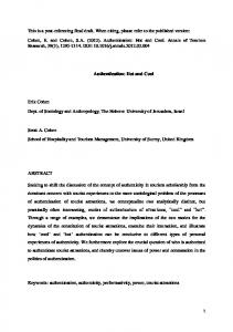
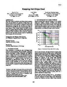
The case presented below used as an exam case in August 2009 for a group of 20 BSc students during their time-constrained double-course exam of the introductory SD course and the introductory differential equations course. The case is about half the size and about half as difficult as a regular introductory SD exam (to compensate for the double-course aspect of the exam). Students found this case easy. Most students were familiar with epidemiological modelling since most of them solved the ‘Cholera in Zimbabwe’ case (Pruyt 2009d) during one of the computer labs. The Pneumonic Plague case description can be found in appendix A on page 22. It is included in the SD exercises book as an exercise at the end of the ‘easy SD questions’ chapter. The basic Pneumonic Plague model is available at http://forio.com/simulate/simulation/e.pruyt/lungpest-in-china). [Case questions 1 and 2:] First students are required to make a simple System Dynamics simulation model (see Figure 1(a)) of a local pneumonic plague epidemic, as well as a corresponding complete ‘causal loop diagram’ (see Figure 1(b)). [Case question 3:] They need to simulate the model and make graphs of the evolution of the infections, the deaths, the recovering population, and the deceased population (see Figure 1(c)). [Case question 4:] Then they need to extend the model to take the social dynamics during an outbreak of an extremely contagious and lethal illness such as pneumonic plague into account: in this case that means an automatic drop in the contact rate caused by illness and anxiety (see Figure 2(a)), and make graphs of the evolution of the infections, the deaths, the recovering population, and the deceased population (see Figure 2(b)). They also need to recognise that the dynamics changes a little bit, but that this does not change the overall picture. [Case question 5 and 6:] Students then have to validate the model and test the sensitivity of the model for small changes in the normal contact rate, the impact of the infected fraction on the contact rate, and another variable of choice. [Case questions 7 and 8:] Finally they need to test whether an increasing supply of antibiotics leads to a lower number of fatalities (see Figure 2(c)) and whether the epidemics can be stopped. Building blocks addressed in this case include stock-flow modelling and causal loop diagramming of aging chains, formulating special functions (lookup functions and time series), and exploring model and policy behaviour. 7 The corresponding SD models and answers will be sent upon request to colleagues willing to exchange ‘hot’ cases. All models are available in Vensim and in Powersim formats, all cases are available in Dutch and English.


(a) Stock-Flow Diagram of the basic Pneumonic Plague model

(b) Causal-Loop Diagram of the basic Pneumonic Plague model

(c) Behaviour of the basic Pneumonic Plague model

Figure 1: SFD, complete CLD and behaviour of the basic Pneumonic Plague model

6


7

(a) Stock-Flow Diagram of the extended Pneumonic Plague model

(b) Behaviour of the extended Pneumonic Plague model

(c) Behaviour of the extended Pneumonic Plague model in case of a linear increase of the antibiotics coverage

Figure 2: SFD and behaviour of the extended Pneumonic Plague model, without/with supply of antibiotics


8

In teaching, this case is used at the end of week 2 (see curriculum in (Pruyt et al. 2009)) or at the end of day one of a three-day workshop.


5

9

Case 2: Mexican Flu

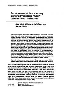
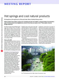
Exploratory SD models of the spread of the new (A/H1N1)v flu variant –also called Mexican flu or swine flu– were developed several days after the first signs of the outbreak of a new flu variant in Mexico. Several months later, the models were used to make a good hot teaching/testing case for BSc and MSc students. The case is good because of the step-wise approach and the familiarity of students with the topic. At Delft University of Technology, the case was given in August 2009 to about 25 BSc students during their time-constrained retake exam of the introductory SD course and in October 2009 to about 35 MSc students during their time-constrained exam. Students found this case relatively easy to solve but complained about the amount of time allotted (3 hours for answering 20 MultipleChoice Questions as well as this case). Nevertheless, students performed –in general– very well on this case. The Mexican Flu case description can be found in appendix B on page 23. The model is extended, explained and explored at length in (Pruyt and Hamarat 2010a), and used to illustrate ESDMA for informed crisis management in (Pruyt and Hamarat 2010b). The basic version of the model is available at http://forio.com/simulate/simulation/e.pruyt/mexican-flu. [Case questions 1.1-1.3:] First, students need to make a very simple simulation model about a flu epidemic in the Western world (see Figure 3(a)), construct a complete CLD of the simulation model (see Figure 3(b)), simulate its behaviour and draw graphs of the evolution of the susceptible population, the infections, the infected fraction, and the recovered population (see Figure 3(c)). [Case questions 2.1-2.2:] Second, students need to extend the simple model displayed in Figure 3(a) with a form of seasonal immunity. Although the extension is rather small, an additional flow (with a well-thought-out formulation8 ) and a time series or sinus function are required. Students are asked to adapt the model and simulate it (see Figure 4(a)), draw graphs of the evolution of the susceptible population, the infections, the infected fraction, and the recovered population (see Figure 4(b)), and compare the outputs of this model with the outputs of the previous model. The epidemic now occurs later and is less catastrophic. [Case questions 3.1-3.2:] Third, students are asked to duplicate the model and turn it into a biregional model comprising the Western world as well as the densely populated Developing World (see Figure 5(a)). Again, students are asked to simulate the model, make graphs of the evolution of the susceptible population, the infections, the infected fraction, and the recovered population of the Western World (see Figures 5(b) and 5(c)), and compare the graphs of the Western region with the previous ones. Students are expected to note that an early outbreak in the Developing World –because of a higher contact rate and a higher infection ratio in the Developing World– may actually lead to an early outbreak in the Western World, but with a lower infected fraction, followed by a more intensive outbreak in winter (when immunity is lower). [Case questions 3.3-3.4:] Then students are asked to validate the model, investigate the sensitivity of the infected fraction of the Western World to small changes of contact rate, infection ratio, and recovery time of the developing world (see Figure 6(a)), and draw conclusions. Possible conclusions are that the infected fraction may not reach the feared third of the population, that the precise outbreak in the developing world may actually lead to a weaker or stronger second peak in the Western world, and that the size of the second peak is inversely proportional to the size of the first peak (which is not the case for other sets of parameter values). [Case question 3.5:] Students are also asked to investigate what happens in terms of the infected population in the Western World if a vaccine becomes available in month 6 and 50% of the Western population gets vaccinated almost immediately after the vaccine has been developed. 8 The flow between these populations, the net ‘susceptible to immune population flow ’ is equal to: (‘normal immune population’ - ‘immune population’)/‘susceptible to immune population delay time’, but the flow cannot be greater than the ‘susceptible population’ divided by the ‘susceptible to immune population delay time’ if there is a net flow towards the immune population, and the return flow cannot be greater than the ‘immune population’ divided by the ‘susceptible to immune population delay time’ if there is a net flow towards the susceptible population.


(a) SFD of the first version of the simulation model of the Mexican Flu case

(b) Complete CLD of the first version of the simulation model of the Mexican Flu case

(c) Behaviour of four key variables for the first version of the Mexican Flu model

Figure 3: SFD, complete CLD, and behaviour of the first version of the Mexican Flu model

10


(a) SFD of the second version of the simulation model of the Mexican Flu case

(b) Behaviour of four key variables for the second version of the Mexican Flu model

Figure 4: SFD and behaviour of the second version of the Mexican Flu model

11


12

(a) SFD of the third version of the simulation model of the Mexican Flu case

(b) Behaviour of four key variables for the third version of the Mexican Flu (c) Detail: the infected fraction model

Figure 5: SFD and behaviour of the third, bi-regional, version of the Mexican Flu model Figure 6(b) shows that one of the consequences for the infected population in the Western World is the elimination of the second outbreak. [Case question 3.6:] Finally, students are asked to formulate a 1-sentence policy recommendation to the European Commission concerning this flu and what to do about it. Students could then for example conclude that: If a vaccine can be made before the second peak, then a heavy first outbreak should be avoided (e.g. by taking the necessary social measures), but if a vaccine cannot be made before the second peak is likely to occur, then it would even make sense to amplify the first peak (e.g. by organising flu parties). Building blocks addressed in this case include stock-flow modelling and causal loop diagramming of aging chains, formulating special functions (lookup functions, time series and/or sinus functions, MIN/MAX functions, well-thought-out flows), and exploring different model and policy behaviours. In teaching, this case is used at the end of week four (see curriculum in (Pruyt et al. 2009)) or at the end of day two of a three-day workshop.


13

(a) Sensitivity of the infected fraction of the Western World to changes in the infected fraction of the Western World to small changes of contact rate, infection ratio, and recovery time of the developing world

(b) Effect of sufficient vaccination before the second flu peak

Figure 6: Sensitivity and policy analyses


6

14

Case 3: The Concerted Run on the DSB Bank

An exploratory SD model of a concerted bank run was developed on 1 October 2009, right after Pieter Lakeman’s call for a run on the DSB Bank. This small, simple, high-level, fast-to-simulate model was used at that time for the purpose of exploration, more precisely, to quickly foster understanding about the possible mechanisms and dynamics of concerted bank runs, to test highlevel policies to prevent such bank runs from succeeding, and to test and teach SD students. The case was given in January 2010 to about 70 BSc students and in November 2009 to about 25 first-year MSc students during their time-constrained introductory SD retake exam at Delft University of Technology. All Dutch students were already familiar with the highly mediatised run on the DSB Bank. Students even guessed –while discussing potentially interesting exam cases during the final lecture– this would be an exam case. Moreover many students had already modelled the similar Fortis Bank case during the computer labs. And although this case is smaller than most hot teaching/testing cases, students found it rather demanding because of the lack of a step-wise approach and somewhat difficult formulations. The DSB Bank Run case description can be found in appendix C on page 25. The model is explained and explored in depth in (Pruyt and Hamarat 2010a), is available and can be simulated at http://forio.com/simulate/simulation/e.pruyt/dsb, and is used briefly for ESDMA in (Pruyt 2010c).

Figure 7: Aggregated structure of a ‘concerted bank run’ SD model [Case question 1:] First, students need to make a simulation model based on the case description. The SFD of the SD model is displayed in Figure 7. Since the model is a short-term crisis


15

model, it is assumed that (i) there is no change in assets due to profit accumulation, (ii) fixed and guaranteed deposits and loans do not come at terms, (iii) there are no net shifts from liquid to fixed assets, nor from liquid to fixed deposits and loans. Note that soft –but possibly important– aspects like anger and expected hindrance from bank failures are explicitly modelled.

Figure 8: Behaviour of different scenarios for the ‘concerted bank run’ model [Case questions 2, 3, 4:] Then students need to use to model to simulate distinct scenarios. Figure 8 shows the behaviours of 4 scenarios on two important variables: the liquid deposits and loans lost and the perceived likelihood of a bank failure. The DSB0 scenario (displayed in green) shows that –with this model and these parameter values (anger amounting to 50%, expected hindrance of a bank failure to 50%, and a liquidation premium of 15%)– nothing happens without a call for a bank run. The DSB1 scenario (displayed in blue) shows that with a concerted bank run lasting two days, 50% anger, 50% expected hindrance of a bank failure, and a liquidation premium of 15%, the initial concerted run is followed by a relatively long period of liquid deposits and loans losses reducing the liquid assets (being replenished by liquidation of fixed assets), before the bank suddenly collapses. The DSB2 scenario (displayed in orange) shows that this collapse occurs sooner with a liquidation premium of 25%. And the DSB3 scenario (displayed in red) shows that the concerted bank run is followed immediately by a full collapse of the bank in case of 100% anger, 100% expected hindrance of a bank failure, and a liquidation premium of 25%. Although the modelled bank seems to collapse sooner or later after an initial perturbation of sufficient amplitude, the delay with which the second run follows upon the concerted run makes a big difference for those involved: in scenarios DSB1 and DSB2 there seems to be some time for strategies/policies and anticipative crisis management, but not in scenario SDB3, in which the second run follows immediately upon the first run, in which case there may only be time for reactive crisis management or an ‘emergency measure’ to place the bank under legal restraint. The strange –at least for continuous systems models– peaks in liquid deposits and loans lost arise because the stock of liquid deposits and loans is depleted. [Case questions 6 and 7:] After briefly validating the model, students need to draw a causal loop diagram to communicate the main feedback loops and explain the link between structure and behaviour: the positive liquidity and solvency loops in Figure 9 make that –unless actively stopped– the likelihood of a bank failure keeps on increasing until the bank effectively collapses. [Case question 8:] Finally, students need to design and test policies to prevent the bank from collapsing. Possible policies include inflows into deposits and loans, especially into the fixed deposits and loans, generated (for example) by raising the interest rate on those products, or by attracting new liquid assets through new equity (both policies are depicted in red in Figure 7). Building blocks addressed in this case include stock-flow modelling and causal loop diagramming of highly aggregated structures, formulating special functions (lookup functions, time series and/or double step functions, MIN/MAX functions, well-thought-out flows), and exploring different scenario and policy behaviours.


16

Figure 9: (Aggregated) Causal-Loop Diagram of the concerted DSB Bank Run Case In teaching, this case is used at the end of week four (see curriculum in (Pruyt et al. 2009)) or at the end of day two of a three-day workshop.

7

Case 4: Chasing Rare Minerals/Metals?

The Rare Earth Metals case presented below was inspired by the first of a series of four articles in Dutch newspapers about scarcity of Minerals/Metals. The case was used on 19 January 2010 to test 15 MSc and 60 BSc students during their time-constrained introductory SD exam at Delft University of Technology. Almost all students found this case extremely difficult because (i) all variables are looped (which means that students using Powersim get error messages in all variables until all problems are solved), (ii) the case is slightly larger than most teaching cases, (iii) more special functions (lookups, time series, Min/Max functions, etc.) need to be formulated, and (iii) the wording was/is not perfect. The case description can be found in appendix D on page 27. A much better –but larger and more complex– SD model related to this topic is described and used in (Pruyt 2010b). [Case questions 1.1 and 1.2:] First, students need to make an incomplete simulation model about the extraction/use/recycling of these metals (see Figure 10(a)), and draw a detailed causal loop diagram of this incomplete model (see Figure 10(b)). [Case question 2.1:] Then students are asked to complete the simulation model by adding structures and variables related to the intrinsic demand, price-driven demand, the demand for recycling, etc (see Figure 11), to simulate the model, and make graphs of the expected price-driven demand, the relative price, the reserves, and an output indicator fraction supplied of intrinsically demanded (see Figure 12). [Case questions 2.2 and 2.3:] Then students need to validate and test the sensitivity of the model (more specifically the fraction delivered of intrinsically demanded and the reserves) for small changes in the price effect supply shortage, the initial reserves, and the fraction available of desired recycling. [Case questions 2.4 and 2.5:] Finally, students are asked to make an aggregated CLD to show the main feedback loops (see Figure 13), and explain the link between structure and behaviour. Building blocks addressed in this case include stock-flow modelling and causal loop diagramming of aging chains and recycling structures, formulating (too) many special functions (lookup


17

(a) Stock-Flow Diagram of the Incomplete Metal Scarcity Model

(b) Detailed Causal-Loop Diagram of the Incomplete Metal Scarcity Model

Figure 10: Stock-Flow Diagram and Detailed Causal Loop Diagram of the Incomplete Metal Scarcity Model


Figure 11: Stock-Flow Diagram of the Metal Scarcity Model

Figure 12: Behaviour of the Metal Scarcity Model

18


19

Figure 13: Aggregated Causal Loop Diagram of the Metal Scarcity Model functions, time series, MIN/MAX functions, well-thought-out flows, delays, and avoiding simultaneous equations), exploring model behaviour, and aggregating and communicating complex feedback loop structures. In teaching, this case is used at the end of week seven (see curriculum in (Pruyt et al. 2009)) or at the end of day three of a three-day workshop.

8

Conclusions, Lessons Learned, Proposal

All new testing/teaching cases developed over the last two years for the introductory SD course at Delft University of Technology have been based on ‘hot’ issues. Using ‘hot’ cases is a good way to enthuse students and to arouse their interest in applying SD in case of real-world issues. Applying SD to ‘hot’ issues illustrates the relevance of SD for dealing with real-world complex issues, which takes SD testing/teaching models one step further than being didactically responsible exercises. Although actual real-world testing/teaching cases are often more motivating, mostly they are also more difficult than exercises developed in the first (and only) place to test/teach, because they need to be sufficiently close to reality to be relevant. Hence it helped to bridge the gap between the introductory SD course and the SD project course by raising the level of difficulty of the introductory SD course. Now students learn all basic SD modelling skills where they ought to learn those skills: in the introductory course. However, developing relatively simple, actual, relevant, real-world testing/teaching cases is very time consuming and difficult, especially when they need to be developed very rapidly in order to be as actual as possible. These ‘hot’ cases have reinforced the reputation of the introductory SD course at Delft University of Technology of being difficult, but also clarified its relevance and goals. Consequently, students seem to work harder and in a more focussed way, and with a side-long glance at the actuality and real-world issues. After only 7 weeks, students are able to construct and use models of real-world issues of a reasonable complexity, be it based on a precise description / specification.


20

The use of ‘hot’ cases may well be the main cause of a significant improvement of the SD modelling skills: although it is difficult to prove, it seems that the use of these testing/teaching cases has accomplished more than the other measures discussed in (Pruyt et al. 2009). In order to maximise the advantages and minimise the disadvantages of using ‘hot’ cases, it is proposed to: • start up a small (informal) network of university-level lecturers interested in sharing ‘hot’ testing/teaching cases, • start exchanging cases bilaterally or by means of a central ‘case depository’, • agree upon a set of criteria (e.g. hot) and a specific standard/format (e.g. italics for variables), • respect authorship and correctly reference/cite (e.g. ‘developed by’ or ‘based on a case developed by’) even for testing cases. Regarding the cases discussed in this paper and provided in the appendix, it can be concluded that: • The Pneumonic Plague case is a rather simple case which is appropriate a 1-1.5-hour exam without multiple choice questions. • The Mexican Flu case is an interesting gradual, relatively easy case which is appropriate for a 2-3-hour exam without multiple choice questions. • The concerted DSB Bank Run case is a relatively difficult case which is appropriate for a 2-2.5-hour exam without multiple choice questions. • The scarcity of minerals/metals case is a difficult case which may be appropriate for a 3-hour exam without multiple choice questions for good/intermediate/advanced SD students.

References Ford, A. (1999). Modeling the environment: an introduction to system dynamics models of environmental systems. Washington (D.C.): Island Press. 3 Meijer, W., E. Pruyt, and J. Slinger (2010, July). Hop, Step, Step and Jump towards Real-World Complexity at Delft University of Technology: A Case of Urban Decay. In Proceedings of the 28th International Conference of the System Dynamics Society, Seoul, Korea. 1, 3 Pruyt, E. (2008a, July). Dealing with multiple perspectives: Using (cultural) profiles in System Dynamics. In Proceedings of the 26th International Conference of the System Dynamics Society, Athens, Greece. System Dynamics Society. 4 Pruyt, E. (2008b, July). Food or energy? Is that the question? In Proceedings of the 26th International Conference of the System Dynamics Society, Athens, Greece. System Dynamics Society. 5 Pruyt, E. (2009a, July). Cholera in Zimbabwe. In Proceedings of the 27th International Conference of the System Dynamics Society, Albuquerque, USA. System Dynamics Society. http://www.systemdynamics.org/conferences/2009/proceed/papers/P1357.pdf. 4 Pruyt, E. (2009b, July). The Dutch soft drugs debate: A qualitative System Dynamics analysis. In Proceedings of the 27th International Conference of the System Dynamics Society, Albuquerque, USA. System Dynamics Society. http://www.systemdynamics.org/ conferences/2009/proceed/papers/P1356.pdf. 4


21

Pruyt, E. (2009c, July). Making System Dynamics Cool? Using Hot Testing & Teaching Cases. In Proceedings of the 27th International Conference of the System Dynamics Society, Albuquerque, USA. System Dynamics Society. http://www.systemdynamics.org/ conferences/2009/proceed/papers/P1167.pdf. 1, 4 Pruyt, E. (2009d, July). Saving a Bank? The Case of the Fortis Bank. In Proceedings of the 27th International Conference of the System Dynamics Society, Albuquerque, USA. System Dynamics Society. http://www.systemdynamics.org/conferences/2009/proceed/papers/ P1273.pdf. 4, 5 Pruyt, E. (2010a). How to Become a System Dynamics Modeller? Hop Step and Jump Towards Real-World Complexity. Delft: Delft University of Technology. (forthcoming – based on current SPM2313 exercises book). 4 Pruyt, E. (2010b). Scarcity of minerals and metals: A generic exploratory system dynamics model. In Proceedings of the 28th International Conference of the System Dynamics Society, Seoul, Korea. System Dynamics Society. http://www.systemdynamics.org/cgi-bin/ sdsweb?P1268+0. 4, 16 Pruyt, E. (2010c, July). Using Small Models for Big Issues: Exploratory System Dynamics for Insightful Crisis Management. In Proceedings of the 28th International Conference of the System Dynamics Society, Seoul, Korea. System Dynamics Society. http: //www.systemdynamics.org/cgi-bin/sdsweb?P1266+0. 2, 14 Pruyt, E. et al. (2009, July). Hop, step, step and jump towards real-world complexity at Delft University of Technology. In Proceedings of the 27th International Conference of the System Dynamics Society, Albuquerque, USA. System Dynamics Society. http: //www.systemdynamics.org/conferences/2009/proceed/papers/P1140.pdf. 1, 2, 8, 12, 16, 19, 20 Pruyt, E. and C. Hamarat (2010a). The concerted run on the DSB Bank: An Exploratory System Dynamics Approach. In Proceedings of the 28th International Conference of the System Dynamics Society, Seoul, Korea. System Dynamics Society. http://www.systemdynamics. org/cgi-bin/sdsweb?P1027+0. 4, 9, 14 Pruyt, E. and C. Hamarat (2010b). The Influenza A(H1N1)v Pandemic: An Exploratory System Dynamics Approach. In Proceedings of the 28th International Conference of the System Dynamics Society, Seoul, Korea. System Dynamics Society. http://www.systemdynamics. org/cgi-bin/sdsweb?P1389+0. 4, 9 Slinger, J., J. Kwakkel, and M. van der Niet (2008, August). Does learning to reflect make better modelers? In Proceedings of the 26th International Conference of the System Dynamics Society, Athens, Greece. System Dynamics Society. 1 Sterman, J. (2000). Business dynamics: systems thinking and modeling for a complex world. Irwin/McGraw-Hill: Boston. 3


22

APPENDIX – APPENDIX – APPENDIX – APPENDIX A

Pneumonic Plague in China

On 3 August 2009, an outbreak of pneumonic plague in north-west China was reported in the media. The NRC Handelsblad (a Dutch quality news paper) reported the following:

The BBC reported: “A second man has died of pneumonic plague in a remote part of north-west China where a town of more than 10,000 people has been sealed off. [. . . ] Local officials in north-western China have told the BBC that the situation is under control, and that schools and offices are open as usual. But to prevent the plague [from] spreading, the authorities have sealed off Ziketan, which has some 10,000 residents. About 10 other people inside the town have so far contracted the disease, according to state media. No-one is being allowed [to] leave the area, and the authorities are trying to track down people who had contact with the men who died. [. . . ] According to the WHO, pneumonic plague is the most virulent and least common form of plague. It is caused by the same bacteria that occur in bubonic plague – the Black Death that killed an estimated 25 million people in Europe during the Middle Ages. But while bubonic plague is usually transmitted by flea bites and can be treated with antibiotics, [pneumonic plague, which attacks the lungs, can spread from person to person or from animals to people], is easier to contract and if untreated, has a very high case-fatality ratio.” You are asked to make an exploratory System Dynamics model of this outbreak. Use the following assumptions: The total population of Ziketan amounted initially to 10000 citizens. New infections make that citizens belonging to the susceptible population become part of the infected population, which initially consists of just 1 person. The number of infections equals the product of the infection ratio, the contact rate, the susceptible population, and the infected fraction. Initially, the normal contact rate amounts to 50 contacts per week and the infection ratio to a staggering 75% per contact. The infected fraction equals of course the infected population over the sum of all other subpopulations. If citizens from the infected population die, they enter the statistics of the deceased population, else they are quarantined to recover. The recovering could be modelled simplistically as (1 − f atality ratio) ∗ inf ected population/recovery time. Suppose for the sake of simplicity that the average recovery time and the average decease time are both 2 days. The fatality ratio depends on the antibiotics coverage of the population which –in this poor part of China– is (initially) 0%. As indicated in the article, the fatality ratio decreases from 90% at 0% antibiotics coverage of the population to 15% at 100% antibiotics coverage of the population. Assume for the sake of simplicity that the recovering population does not pose any threat of infection, either because they are is really quarantined or because they they are not contagious any more. 1. Make a System Dynamics simulation model of a local pneumonic plague epidemics. Verify the model.


23

2. Make a ‘causal loop diagram’ of this model. 3. Simulate the model using a time horizon of a month. Make graphs of the evolution of the infections, the deaths, the recovering population, and the deceased population. 4. The outbreak of an extremely contagious deadly illness such as pneumonic plague actually causes the contact rate to drop (because of panick and illness). Adapt the model by closing the ‘loop’ between the infected fraction and the contact rate. Create a function impact of the infected fraction on the contact rate that, multiplied with the aforementioned normal contact rate (the one without epidemic and panick), gives the effective contact rate. The function takes a value of 1 at an infected fraction of 0% 1, of 0.5 at an infected fraction of 10%, of 0.25 at an infected fraction of 20%, 0.125 at an infected fraction of 30%, of 0.0625 at an infected fraction of 40% , of 0.03125 at an infected fraction of 50%, and so on. Simulate the model over a span of 1 month. Make graphs of the evolution of the infections, the deaths, the recovering population, and the deceased population. Does this reduction of the natural contact rate the desired effect? 5. Validate your model. Propose 2 validation tests (except sensitivity analysis – see next question), perform them, and briefly describe the results/conclusions. 6. Test (not too extensively) the sensitivity of the model for small changes in the normal contact rate, the impact of the infected fraction on the contact rate, and one other variable of choice. Briefly describe your conclusions. 7. Suppose that the antibiotics coverage of the population increases linearly in de first week of the epidemics from 0% to 100%. What is the consequence on the deceased population? 8. Could the epidemics be stopped? Explain based on the structure of the model.

B

Mexican Flu

Mexican flu epidemic or pandemic: does it matter? Let’s go several months back in time to the moment the WHO reported the first signs of the Mexican flu outbreak. Suppose that the European Commission asked you at that time to make an experimental System Dynamics model related to the potential evolution of the Mexican Flu (also known as A/H1N1 or swine flu) in the Western World. Model and analyse the Mexican flu, first as an epidemic in the Western World, and then, as a worldwide epidemic or pandemic in the Western World and the densely populated part of the developing world. Keep in mind during your analyses that the Western World was especially concerned about potential disruptions of society and economy if more than 30% of the active population simultaneously has the flu.

B.1

Mexican flu as an epidemic in the Western World (

/7.5)

Infections make that people from the susceptible population (initially equal to 600.000.000 persons) get the flu and migrate from the susceptible population to the infected population (initially equal to 10 persons). The number of infections equals the product of the susceptible population, the contact rate, the infection ratio, and the infected fraction. The infected fraction equals the infected population divided by the total population. The average infection ratio of this flu variant in the Western World was estimated at that time to amount to 10% infections per (close) contact. Suppose that the contact rate in de Western World amounts to 50 (close) contacts per person per month. Members of the infected population flow after an average recovery time of 2 weeks to the recovered population (initially empty). Assume for the sake of simplicity that the entire infected


24

population recovers (although feared at first, there are, relatively speaking, not that many swine flu deaths). 1. ( /3) Make a System Dynamics simulation model in Powersim of Vensim of the epidemic described above. Verify the model. 2. ( /3) Make a complete causal loop diagram of this simulation model. 3. ( /1.5) Simulate the model over a period of 4 years. Make graphs of the evolution of the susceptible population, the infections, the infected fraction, and the recovered population.

B.2

What if not everyone in the Western World is infected? (

/5.5)

It is likely that not everyone gets this flu, just like in case of the normal flu. That probably means that there is –apart from the susceptible population– also an immune population. Adapt the previous model. Set the susceptible population in the Western World initially to 330.000.000 persons and the immune population to 270.000.000 persons. However, there is also a seasonal dynamic between both populations: the susceptible population grows towards the winter season, and the immune population grows towards the summer season. The flow between these populations, the net ‘susceptible to immune population flow ’ is equal to: (‘normal immune population’ - ‘immune population’)/‘susceptible to immune population delay time’, but the flow cannot be greater than the ‘susceptible population’ divided by the ‘susceptible to immune population delay time’ if there is a net flow towards the immune population, and the return flow cannot be greater than the ‘immune population’ divided by the ‘susceptible to immune population delay time’ if there is a net flow towards the susceptible population. Suppose that the ‘susceptible to immune population delay time’ amounts to 1 month. The normal immune population is equal to the product of the total population and the normal immune population fraction. This normal immune population fraction fluctuates between 30% in month 0, to 70% in month 6, to 30% in month 12, to 70% in month 18, and so on. 1. ( /3.5) Extend the simulation model as described above. 2. ( /2) Simulate the model over a period of 4 years. Make (on your computer and on your exam copy) graphs of the evolution of the susceptible population, the infections, the infected fraction, and the recovered population. Compare these graphs with the previous ones: briefly describe the differences.

B.3

The Mexican flu as a worldwide epidemic (or pandemic)? (

/12)

[Remark: You can model the description in this subsection, even if unsuccessful in subsection B.2.] The flu epidemic in the Western World may be strongly influenced by the development of the flu in densely populated Developing Countries. Make therefore a similar submodel for a second region, namely the densely populated part of the third world. There are some small differences: Suppose that the average contact rate in this second region amounts to 100 (close) contacts per person per month. The infection ratio is probably slightly higher, namely 15% or 0.15 infections per contact. The susceptible population of this region amounts initially to 2.000.000.000 persons, the immune population to 1.000.000.000 persons, and the infected population to 100 persons. [Scarcely populated regions are not modelled here because they are causally less important to an outbreak of the flu.] The majority of these countries are located in the Southern hemisphere, and their populations generally have a lower immunity: the normal immune population fraction amounts therefore to 30% in month 0, 10% in month 6, 30% in month 12, 10% in month 18, and so on. There is of course also contact between these regions (the Western World and the densely populated Developing Countries). Suppose that the interregional contact rate amounts to 0.1


25

(close) contacts per person per month. Add an additional term to the infections variables of both regions. In case of region 1, this additional term may look like: + ‘susceptible population region 1 ’ x ‘interregional contact rate’ x ‘infection ratio region 1 ’ x ‘infected fraction region 2 ’ 1. ( /4) Extend the simulation model as described above. 2. ( /1.5) Simulate the model over a period of 4 years. Make (on your computer and on your exam copy) graphs of the evolution of the susceptible population, the infections, the infected fraction, and the recovered population of the Western World. Compare the graphs of the Western region with the previous ones: briefly describe the differences. 3. ( /1) Validate the model: propose 2 validation tests (except sensitivity analysis), perform them, and briefly describe the resultats/conclusions. 4. ( /3) Investigate the sensitivity of the Western World submodel to small changes of contact rate, infection ratio, and recovery time of the Developing Countries. Test for example a contact rate in region 2 of 200 (close) contacts per person per month. Describe briefly what you can conclude from these analyses in terms of the infected fraction of the Western World. 5. ( /1.5) Suppose that a vaccine becomes available in month 6 and that 50% of the Western population gets vaccinated in no time. What is the consequence in terms of the evolution of the infected population in the Western World? 6. ( /1) Formulate a 1-sentence policy recommendation concerning this flu and what to do about it to the European Commission.

C

A Concerted Run on the DSB Bank

Over the last year, newspapers have been reporting about many bankruptcies of banks and financial institutions. The latest bankruptcy of a Dutch bank, the Dirk Scheringa Bank or DSB, is a very special case, because the bankruptcy was actually caused by a concerted bank run by angry clients following the call by Pieter Lakeman to empty their deposits. Since you already modelled the fall of the Fortis Bank, you are asked by the Dutch central bank ‘De Nederlandse Bank ’ to model the fall of the DSB. Keep in mind that a crisis model is not the same as a complete bank model for going concern. Deposits being emptied are –from the point of view of a bank– liquid deposits and loans lost. These liquid deposits and loans lost drained the liquid deposits and loans, which initially amounted to e4,500,000,000. Liquid assets lost are equal to the liquid deposits and loans lost because of the double accounting system. Liquid assets lost decrease the amount of liquid assets, which initially amounted to e1,150,000,000. Suppose that there is a liquid asset liquid liability target of 20%, which means that fixed assets, which initially amounted to e4,600,000,000), need to be liquidated and turned into liquid assets if less than 20% of liquid deposits and loans are covered by liquid assets. Suppose that the liquidation time is only 1 day, which means that there are enough interested parties to almost instantly sell assets to. However, given this haste, there is a liquidation premium of 10% on these emergency sales. In other words, only 90% of the fixed asset value is turned into liquid assets in these emergency sales, and 10% of the fixed asset value is lost as liquidation losses. Keep in mind when you model the liquidation flow that the model you make is a crisis model and not a complete banking model: there should at most be a net flow from fixed assets to liquid assets, but not the other way around. Apart from the liquid deposits and loans, DSB also had fixed deposits and loans worth e1,000,000,000 which remained constant during the crisis because fixed deposits and loans cannot be emptied by depositors or lenders before their due date.


26

In a normal bank run, the amount of liquid deposits and loans lost equals the liquid fraction running away away times the liquid deposits and loans divided by the withdrawal time. However, two factors amplified the running away effect in the case of DSB crisis: clients were angry because of unacceptable sales practices and the mediatised unwillingness of the bank to compensate the victims of these practices, and people understood the hindrance of a bank failure9 after having witnessed bankruptcies of several banks over the past few months. Multiply the previous right hand side of the equation therefore with following two factors: (1+hindrance of bank failures) and (1+anger ). Suppose that the hindrance of bank failures amounts to 0.5. Since the DSB bank run was actually to some extent an organised bank run, you have to add an additional term to take this concerted action into account, for example: concerted liquid fraction running away times liquid deposits and loans divided by withdrawal time of 1 day. And do not forget that the maximum amount of liquid deposits and loans lost equals the amount of liquid deposits and loans divided by the withdrawal time. Suppose that the liquid fraction running away amounts to 0% if the perceived likelihood of a bank failure is 0%, that it amounts to 0% if the perceived likelihood of a bank failure is 25%, that it amounts to 1% if the perceived likelihood of a bank failure is 50%, that it amounts to 10% if the perceived likelihood of a bank failure is 75%, and that it amounts to 50% if the perceived likelihood of a bank failure is 100%. The perceived likelihood of a bank failure may be modelled as (100% - credibility of the denials) times the maximum of either the perceived likelihood of a liquidity failure or the perceived likelihood of a solvency failure. Suppose that the perceived likelihood of a liquidity failure amounts to 100% if the liquid asset liquid liability ratio equals -1, that it amounts to 100% if the liquid asset liquid liability ratio equals 0, that it amounts to 80% if the liquid asset liquid liability ratio equals 0.1, that it amounts to 40% if the liquid asset liquid liability ratio equals 0.2, that it amounts to 10% if the liquid asset liquid liability ratio equals 0.3, that it amounts to 1% if the liquid asset liquid liability ratio equals 0.4, that it amounts to 0% if the liquid asset liquid liability ratio equals 0.5, and that it amounts to 0% if the liquid asset liquid liability ratio equals 1. Suppose that the perceived likelihood of a solvency failure amounts to 100% if the total asset total liability ratio equals 0, that it amounts to 100% if the total asset total liability ratio equals 0.8, that it amounts to 90% if the total asset total liability ratio equals 0.9, that it amounts to 50% if the total asset total liability ratio equals 1, that it amounts to 10% if the total asset total liability ratio equals 1.1, that it amounts to 0% if the total asset total liability ratio equals 1.2, and that it amounts to 0% if the total asset total liability ratio equals 2. The liquid asset liquid liability ratio is of course equal to the amount of liquid assets over the amount of liquid deposits and loans. And the total asset total liability ratio equals the sum of the fixed assets and the liquid assets over the sum of the liquid deposits and loans and the fixed deposits and loans. The central bank issues a bank failure declaration (forcing a bank into bankruptcy) if the liquid asset liquid liability ratio falls below 0.05 or the total asset total liability ratio falls below 0.9. 1. ( /8) Make a System Dynamics simulation model of this issue on your computer. Save and verify the model. 2. ( /1) Simulate the model first of all over a time horizon of about 60 days without any anger or an ‘organised’ bank run. In other words, set anger equal to 0, concerted liquid fraction running away away equal 0%, and the credibility of the denials equal to 90%. Make graphs of liquid deposits and loans lost and the perceived likelihood of a bank failure, both on your computer and on this exam copy. 9 Even without losing money (in case of depositor guarantees), depositors have to wait for months to get their money back.


27

3. ( /5) Now, adapt the model to simulate a bank run following Pieter Lakeman’s call for an concerted bank run. Suppose for example that the concerted liquid fraction running away jumps to 5% on day 2 and falls down to 0% on day 4 and that the credibility of the denials falls from 90% to 10% from day 2 on. Suppose also that on top of these changes the variable anger amounts to 0.5 and the liquidation premium to 25%. Save the model using your family name, the number of the question, and the version. (a) Simulate the model over a time horizon of 60 days. Make graphs of liquid deposits and loans lost and the perceived likelihood of a bank failure, both on your computer and on this exam copy. (b) Explain the behaviours obtained, especially if you obtain strange behaviours. (c) Briefly describe whether and what the bank could do to prevent this bank run (do not model it here). 4. ( /3) Simulate a bad case scenario, again over a time horizon of 60 days, in which anger is 1, hindrance of bank failures is 1, and the liquidation premium is 25%. (a) Make graphs of liquid deposits and loans lost and the perceived likelihood of a bank failure, both on your computer and on this exam copy. (b) Briefly describe the differences with the previous behaviour? (c) Briefly describe whether and what the bank could do to prevent this bank run (do not model it here). 5. ( /1) Validate the model extremely briefly. Use maximum 2 (different) validation tests. List the tests used and briefly describe the conclusions of the tests. 6. ( /4) Draw a causal loop diagram of the system to help you communicate the main feedback effects responsible for the bank run. 7. ( /1) Explain the link between structure & behaviour briefly (e.g. for the ‘bad case’ scenario). 8. ( /1) Save your model under another name and add a simple closed loop policy (in colour) that prevents the bank from collapsing. Describe the policy briefly. Test the policy at least in case of the ‘bad case’ scenario and sketch the resulting dynamics on your exam copy. 9. ( /1) How do we call variables like hindrance of bank failures and anger ?

D

Chasing Rare Minerals/Metals?

Rare earth metals are necessary in ever bigger quantities for all sorts of innovative –mostly ‘green’– technologies such as hybrid cars, flat screens, solar cells, led lamps, mobile phones, et cetera. But these metals are, as the name already suggests, rare. Moreover, some countries such as China, which already have quasi-monopolies on the extraction of particular scarce metals, are said to have constrained the export of these rare metals. These natural or artificial constraints may lead to temporary or/and structural scarcity, which in turn may hinder the transition of our society towards a more sustainable one. . . Make a SD model about the dynamics of the extraction and scarcity of a particular –nonspecified– rare metal, ‘metal X’, based on the following description, and simulate it over the period 2000 to 2050.


D.1

28

Extraction, Use and Recycling

Unextracted reserves of metal X, initially equal to 10000t, decrease through extraction with a yearly extraction time of one year. Extraction increases the supply of metal X, initially equal to the initial demand for metal X from 400t per year, and production of metal-X-containing products decreases the supply of metal X stock after an average production time of metal-X-containing products of a year. That increases the quantity of metal X in use, initially equal to 3000t. After an average lifetime of metal X in use of 10 years, part of this quantity of metal X in use is recycled and the rest is lost. This division depends on the recycling fraction of metal X. Initially, there is no metal X in recycling. The annual recycling time of metal X is one year and generates a supply of recycled metal X flow which increases the supply of metal X stock, and determines –together with the expected price driven demand for metal X – the desired extraction of metal X. This desired extraction drives the extraction. 1. Make a preliminary System Dynamics simulation model of this issue. Use, if necessary, first-order delay structures. 2. Make a detailed causal loop diagram of the stock-flow diagram above. How many feedback loops are there?

D.2

Intrinsic demand, price driven demand, recycling demand, etc.

Suppose that the expected intrinsic demand for metal X, initially equal to 400t (see above), increases annually with an expected percentage increase of the intrinsic demand for metal X of 3% per year. Model the expected price driven demand for metal X as a first-order delay of a year –with initial value the expected initial demand for metal X – of the following fraction: expected intrinsic demand f or metalX . relative price metal X The price effect supply shortage of metal X is a graph/lookup function with as argument: expected price driven demand for metal X /production metal X containing products. The desired recycling of metal X equals this expected price driven demand for metal X multiplied with the relative attractivity of recycling versus extraction10 plus the difference between the desired extraction metal X and the real extraction of metal X. The recycling fraction of metal X is equal to the fraction available of desired recycling of metal X times the desired recycling of metal X divided by the maximal recyclable quantity metal X. The latter fraction necessarily needs to be limited at a maximum of 1. The maximal recyclable quantity of metal X equals the quantity of metal X in use which becomes available at the end of the average lifetime of metal X in use of 10 years. Suppose that the fraction available of desired recycling of metal X increases as follows: 10% in 2000, 50% in 2010, 80% in 2020, 89% in 2030, 90% in 2040 at which it stabilises. The effective fraction recycled supply of total supply metal X equals the supply of recycled metal X divided by the sum of the extraction of metal X and the supply of recycled metal X. Suppose that the relative recycling cost of metal X decreases from 10 (so 10 times the normal extraction cost) in 2000, to 2 in 2010, to 1 in 2020, to 0.9 in 2030 at which it stabilises, and that the relative exploitation cost of metal X is a function of the fraction remaining reserves of metal X with values (0, 100), (0.05, 2.5), (0.1, 1.25), (0.15, 1.1), (0.2, 1), (0.25, 1) (in other words, at a fraction of 5% the relative cost is 2.5 times as high as with a fraction of 20% or more). The average cost of metal X is then the weighted average of the relative recycling cost of metal X and the relative exploitation cost van metal X, proportional to the fraction of recycled supply of total supply of metal X. The fraction remaining reserves of metal X is of course equal to the reserves of metal X divided by the initial reserves of metal X. 10 This

relative attractivity could be modelled as:

1 relative recyclingcost of metal X 1 1 + relative recyclingcost relative exploitationcost of metal X metal X

.


29

Suppose now that the market functions such that the relative price of metal X equals the average cost of metal X times the ‘price effect supply shortage of metal X ’. Suppose that this price effect is a function of the demand/supply fraction, or here, of the expected price driven demand for metal X divided by the production of metal X containing products, with values (0, 0.1), (1, 1), (1.5, 2), (2, 10), (5, 100) (in other words, a demand/supply fraction of 5 leads to a 100 times higher price than usual). Also make sure that there is not more extraction than there are non-extracted resources. And add an output indicator to monitor the fraction delivered of the intrinsic demand of metal X. This equals the supply of metal X divided by the expected intrinsic demand for metal X. 1. Extend the simulation model with the information above. Verify the model briefly. Simulate the model and make graphs of the expected price driven demand for metal X, the relative price of metal X, the reserves of metal X, and the output indicator fraction supplied of intrinsic demand for metal X. 2. Validate the model. List 2 validation tests, perform them and describe the results (briefly). 3. Test the sensitivity of the model (more specifically the fraction delivered of intrinsic demand for metal X and the reserves of metal X ) for (small) changes in following functions and parameters: the price effect supply shortage of metal X, the initial reserves of metal X, and the fraction available of desired recycling of metal X. Describe briefly the tests you performed, and your results and conclusions. 4. Make an extremely aggregated causal loop diagram of the model which allows you to explain the main feedback loop effects. 5. Explain the link between system and behaviour (more specifically of the output indicator). D.2.1

Strategic and speculative reserves (BONUS)

When it comes to scarcity of metals, people are scared that strategic and speculative reserves are built, especially by states that already have a quasi-monopoly on the exploitation. 1. Extend the model with a submodel dealing with strategic reserves (for national use, which means they are not available on the world market). Simulate the model and sketch the difference in behaviour. 2. Extend the model with a submodel dealing with speculative reserves (temporarily unavailable on the market to be sold later for a higher price on the market). Simulate the model and sketch the difference in behaviour.

Making System Dynamics Cool II: New Hot Teaching and Testing ...

Making System Dynamics Cool II: New Hot Teaching and Testing ...

Suggest Documents

Making System Dynamics Cool? Using Hot Testing ... - Semantic Scholar

Making Cool Drugs Hot

Making Cool Drugs Hot

Authentication Cool and Hot - Core

Keeping Hot Chips Cool

ITC Making cool drugs hot Holdgate MicroCal app ...

Journal of Vibration Testing and System Dynamics

Journal of Vibration Testing and System Dynamics

Journal of Vibration Testing and System Dynamics

Journal of Vibration Testing and System Dynamics

Journal of Vibration Testing and System Dynamics

Journal of Vibration Testing and System Dynamics

Journal of Vibration Testing and System Dynamics

SySc 610SD2: System Dynamics II

Journal of Vibration Testing and System Dynamics

Cool'' Jobs in ''Hot'' Industries

Hot Stars With Cool Companions

Hot and Cool Executive Functions in Adolescence

Hot springs and cool natural products

Making Steel Cool - Springer Link

Cool Subdwarf Investigations II: Multiplicity

the dynamics of stellar coronae harboring hot jupiters. ii ... - IOPscience

Cool-Cache for Hot Multimedia - CiteSeerX

1 Dyson AM09 Hot + Cool Fan - HubSpot