Malware Detection Using Perceptrons and Support ... - Semantic Scholar

Malware Detection Using Perceptrons and Support Vector Machines Dragos¸ Gavrilut¸1,2 , Mihai Cimpoes¸u1,2 , Dan Anton1,2 , Liviu Ciortuz1 1 - Faculty of Computer Science, “Al. I. Cuza” University of Ias¸i, Romania 2 - BitDefender Research Lab, Ias¸i, Romania Email: {gdt, mcimpoesu, dan.anton, ciortuz}@info.uaic.ro

Abstract—In this paper we explore the capabilities of a framework that can use different machine learning algorithms to successfully detect malware files, aiming to minimize the number of false positives. We report the results obtained in our framework, working firstly with cascades of one-sided perceptron and kernelized one-sides perceptrons and secondly with cascade of one-sided support vector machines. Keywords-Malware detection; perceptrons; Support Vector Machines.

I. I NTRODUCTION Malware is defined as software designed to infiltrate or damage a computer system without the owner’s informed consent. Malware is actually a generic definition for all kind of computer threats. A simple classification of malware consists of: − file infectors, which are viruses that insert their own code in other files; these are usually executable files but other types of files can be affected as well; − stand-alone malware, when the whole regarded file is an application that performs malicious actions. Another way of classifying malware is based on their particular action: − worms, that spread over the network using different system vulnerabilities; − backdoors, that offer the attacker a way to remotely control another computer; − trojans, that masquerade as a legitimate applications and perform different malicious actions on victim’s computer; − rootkits, that hijack some system functions in order to render their malicious files or processes invisible from normal user programs; − spyware, that collect different private information about the victims computer like passwords, credit card numbers, email accounts and contacts; − adware, that display different kind of advertising stuff on the user’s computer. Malware detection through standard, signature based methods is getting more and more difficult since all current malware applications tend to have multiple polymorphic layers to avoid detection or to use side mechanisms to automatically update themselves to a newer version at short periods of time in order to avoid detection by any antivirus software.

Our aim is to overcome some of the big problems that the antivirus technologies face nowadays. Ultimately, these problems are expressed in terms of generic detection of malware, while getting as few false positives as possible. In this paper, we explore the capabilities of a simple framework for malware detection, by using a simple and a layered combination (cascade) of different machine learning algorithms [1]. (Related, machine learning work for malware detection is discussed in Section II.) The main steps performed through this framework are sketched as follows: 1. A set of features is computed for every binary file in the training or test datasets (presented in Section III), based on many possible ways of analyzing a malware. 2. A machine learning system based firstly on the cascade onesided perceptron, a feature mapped perceptron and a kernelized perceptron, and secondly on cascade one-sided Support Vector Machines (SVMs), combined with feature selection based on the F1 and F2 scores, is trained on a medium-size dataset consisting of clean and malware files. Cross-validation is then performed in order to choose the right values for parameters. Finally, tests are performed on another, non-related dataset. The obtained results (see Section V) were very encouraging. II. R ELATED W ORK The problem of detecting generic malware without the classical signature-based procedure led many security researchers towards the field of machine learning and data mining. In their research, a series of methodologies were proposed, however none of these techniques has a strict policy for keeping the number of false positives under control. The use of n-grams is among the best studied approaches to malware detection. An IBM research group proposed this method in 1994, but there were no experimental results in their publication [2]. Furthermore, in 2004 Assaleh et al. provided very good results regarding the detection rate (true positives), but no information about the false positives [3]. They collected n-gram profiles for every file in each class, both malware and clean, and used the k-NN algorithm with k = 1. The lack of false positive ratio in the experimental results and the absence of any technique to control the appearance of false positives render this method unpractical in a commercial way. A very good work using n-grams for malware detection was presented by Jeremy Kolter and Marcus Maloof [4]. They

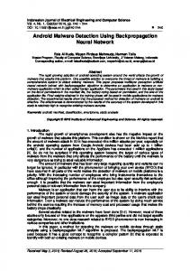
use multiple machine learning algorithms applied on the same characteristics as the two research groups mentioned above. Boosted decision trees and boosted SVM show very promising results with over 99% detection rate and a false positive rate under 0.75%. A very thorough testing methodology is used; they illustrate the detection rate of each algorithm with respect to the corresponding false positive rate using ROC curves. Using n-grams as the characteristics for machine learning in the detection of malware gives good results on small lots or collections targeting specific malware families, but this technique becomes invalid for a general purpose commercial antivirus scanner as the number and diversity of malware individuals gets higher and higher every day. Some non-standard methods for detecting polymorphic malware have been developed over time. In 2004 InSeon Yoo [5] proposed a way of identifying file-infector viruses by using self-organizing maps [6] to take advantage of the executable file structure. In 2006 Ruben Santamarta [7] described a way of extracting static signatures of specific code protectors and packers. He analyses the specifics of the assembly language mnemonics such as the frequency of appearance, the relative frequency or a correlation between them. These specific features of every individual in the targeted family are fed into a neural network that is able to identify a pattern to be later used for detection. However, this type of signature is only useful to identifying targeted malware families, and there is no indication whether this may or may not raise any false positives. We created our own features which regard a targeted file from many possible points of interest. This enables us to control the false positive and malware detection rate by introducing new features or removing some others as needed. Our main target is to have a decent detection rate with a false positive as close as possible to zero. III. DATASETS A training database was created (henceforth denoted VH), which contains 273133 clean files and 27475 malware files. The malware files were collected from the Virus Heaven website. Since our main target was to create a detection with as few as possible (or even 0) false positives, the VH database has much more clean entries than malware ones. The malware files in this collection are of a variety of types such as: trojans, backdoors, hacktools, rootkits, worms and other types, as shown by the graph given in Figure 1. The clean files from the training (VH) database are mainly system files (from different versions of operating systems) and executable and library files from different popular applications. We also use clean files that are packed or have the same form or certain geometrical similarities with malware files (e.g. use the same packer) in order to better train and test our machine learning system. From the whole set of feature we created, 308 binary features were selected. Different files may generate equal sets of values for the chosen feature set; therefore they were counted only once. For the training (VH) dataset, the total

Fig. 1. Malware distribution in the training (VH) dataset. Each one of the left columns represents the percentage of that malware family from the total number of files, while each one of the right columns represents the corresponding percentage from the total number of unique combinations of features.

Fig. 2. Malware distribution in the test (WL) dataset, showing the percentage of different types of malware with respect to the total number of malware files.

number of unique combinations of the selected features was 8237 (7822 malware combinations and 415 clean combinations). The number of clean combinations is much smaller than the malware ones because most of the features were created to emphasize a specific aspect of malware files (either a geometrical form or a behavioural aspect of the malware). A second dataset (henceforth denoted WL) was created for testing the models obtained through training. It contains a smaller set of malware files (from the Wildlist collection) and clean files selected from different operating systems (other files that the ones used in the training, VH database). The total number of malware files that were used for the test (WL) database is 11605. The total number of clean files in this dataset is 6522. The total number of unique combinations for this database is 636 (506 malware combinations and 130 clean combinations). The distribution of each malware type in this dataset is shown in Figure 2 and, as it can be seen, is different from the distribution in the training (VH) dataset. IV. F EATURES For every binary file in the training and test datasets, a set of features/attributes was computed, based on many possible

ways of analyzing a malware, for instance: • behaviour characteristics in protected environments, 1 • file characteristics from the PE format point of view, • file format from a geometrical point of view, • file packer, obfuscator or protector type, • package installer type, • file content information retrieved from imports, exports or resource directory or from different strings that reside in the data section of the file. The total number of file attributes that we defined is around 800, but for the somehow restricted scope of this paper we only used 308 boolean attributes. For further formalisation, we define our data structures as follows:

Fig. 3. F1 and F2 scores values for the chosen 308 features computed on the training (VH) dataset.

F = (fa1 , fa2 , . . . , fan ) is the set of attribute values that characterize a file, each ai being a file attribute. Ri = (Fi , labeli ) is a record; labeli is a boolean value that identifies the file that has attributes Fi as being either a malware or a clean file. R = (R1 , R2 , . . . Rm ) is the set of records for all the training files that we use. Starting from the set of the chosen 308 features, we also created another set of features, by explicitly mapping the original features into a larger space as follows. ′ ′ ′ We define F ′ = (fa1 , fa2 , ..., fam ), where m = n(n + 1)/2 ′ and fa k = fa i &fa j , i = [k/n] + 1, j = [k%n] + 1, k = [1 . . . m], with & denoting the logical conjunction operation. The number of resulted features in F ′ will be n(n + 1)/2, where n is the number of features in F . The computational time increases heavily, e.g. for the 308 features in F , we will have 47278 features in F ′ . However, our results have shown that the detection rate at cross-validation increases with about 10% when computed on F ′ compared to F . For the implicit mapping of the training instances into a higher-dimension space, the following kernel functions will be used in the Section V: − the polynomial kernel: K(u, v) = (1+ < u, v >)d , where < u, v > is the dot product of the u and v vectors; −|u−v|2 − the radial-base function (RBF): K(u, v) = exp( 2×σ2 ). For feature selection we will use the F-scores statistical measures. The “quality” of the ith feature is described commonly by the statistical scores F1 and F2 defined by the equations (1). The larger the values for the ith feature, the more likely this feature possesses discriminative power. F 1i = 1 The

− − 2 2 (µ+ |µ+ i − µi ) + (µi − µi ) i − µi | − , F 2i = − 2 + + 2 |σi − σi | (σi ) + (σi )

(1)

Portable Executable (PE) format regards executable files, object code and DLLs used in 32-bit and 64-bit versions of the MS Windows operating system. The term “portable” refers to the format’s versatility in numerous environments of the operating system’s software architecture. The PE format is basically a data structure that encapsulates the information necessary for the Windows OS loader to manage the wrapped executable code. This includes dynamic library references for linking, API export and import tables, resource management data and thread-local storage (TLS) data.

Fig. 4. Training and testing results obtained with COS-P on the training (VH) dataset through 3-fold cross-validation after F1 and F2 feature selection. Percentages on the horizontal axis: the amount of selected features. On the vertical axis: the sensitivity (SE) value.

− + − The notations µ+ i /µi and σi /σi correspond to the means and standard deviations of the positive (+) and respectively the negative (-) subsets in the training dataset. [8]. Figure 3 suggests that there is an approximate (though nonlinear) correlation between the F1 and F2 scores computed on the training (VH) dataset.

V. R ESULTS We performed training and tests using different perceptron and SVM versions, using the same datasets of files, VH and WL. Each time we computed the number of true positives (TP), the number of false positives (FP), the sensitivity measure value (SE), the specificity (SP), the accuracy measure value (ACC), as defined for instance in [9]. A. Results obtained with perceptrons The results shown in the tables of this subsection were obtained for the following algorithms, which are detailed in [10]: • COS-P – Cascade One-Sided Perceptron. • COS-P-Map-F1 – Cascade One-Sided Perceptron with explicitly mapped features. The algorithm used 30% of the original features given by the best F1 score values and

TABLE I P ERCEPTRON R ESULTS ON THE T EST (WL) DATASET. Algorithm COS-P COS-P-Map-F1 COS-P-Map-F2 COS-P-Poly2 COS-P-Poly3 COS-P-Poly4 COS-P-Radial

TP 356 356 357 455 466 465 264

FP 3 2 2 9 19 20 19

SE 68.73% 83.76% 83.22% 87.84% 89.96% 89.77% 89.13%

SP 97.46% 96.97% 97.14% 92.37% 83.90% 83.05% 86.92%

ACC 74.06% 85.54% 85.17% 88.68% 88.84% 88.52% 88.68%

explicitly mapped them into 1830 new features, as specified in Section IV. It should be taken into account that after selecting the first 30% features, duplicates appeared in the training dataset, and after their elimination, 6580 records remained. • COS-P-Map-F2 – Same as COS-P-Map-F1 with the difference that we sorted the original features by F2; 6644 records remained after duplicate elimination. • COS-P-Poly2/COS-P-Poly3/COS-P-Poly4 – The Cascade One-Sided Perceptron with the polynomial kernel function shown above with the degree of 2/3/4. • COS-P-Radial – The Cascade One-Sided Perceptron with the RBF kernel function with σ = 0.04. The COS-P-Map algorithm uses a lot of features, due to the explicit mapping (see Section IV). This will slow down the training algorithm. That is why we performed feature selection based on the F1 and F2 statistical scores, in order to see whether we can find a subset of features that will produce similar results. We performed 3-fold cross-validation tests on the training (VH) dataset using the COS-P algorithm, and employing the first 10%, 20%, 30% . . . 100% features selected via the F1 and respectively F2 scores. The results are presented in Figure 4, and they show that selecting the first 30% features (by either F1 or F2) will lead to classification results which are similar to those obtained by the COS-P algorithm when using all features. We performed comparative tests for 3, 5, 7, and 10 folds for the COS-P, COS-P-Map, COS-P-Poly and COS-P-Radial algorithms. For each algorithm, we used the best result from maximum 100 iterations, each iteration having two steps. The first step performs training as usual on the data, while the second step iteratively improves the perceptron’s weights on the training data until no clean file is misclassified. The results obtained for the cascade one-sided perceptrons on the test dataset WL (Table I) show that the COS-P-Map algorithm produces the best results with fewer false positives. Both COS-P-Map-F1 and COS-P-Map-F2 algorithms yielded the lowest false positive rate compared to all other algorithms even if the malware distribution in this dataset is different from the one in the training (VH) dataset. From the technical point of view, the most convenient algorithms are COS-P and COS-P-Map. Both have a small memory footprint, a short training time (not shown here), a good detection rate and few false positives.

TABLE II 5- FOLD C ROSS - VALIDATION , SVM R ESULTS ON THE T RAINING (VH) S ET. Algorithm SVM-Map-F1 SVM-Map-F2 SVM-Poly2 SVM-Poly3 SVM-Poly4 SVM-Radial

TP 6149 6179 7728 7741 7744 7747

FP 68 74 94 81 78 75

SE 97.46% 97.66% 97.64% 97.36% 96.99% 97.93%

SP 74.81% 76.58% 70.72% 71.58% 69.05% 76.92%

ACC 96.53% 96.66% 96.59% 96.47% 96.14% 97.10%

TABLE III 10- FOLD C ROSS - VALIDATION , SVM R ESULTS ON THE T RAINING (VH) S ET. Algorithm SVM-Map-F1 SVM-Map-F2 SVM-Poly2 SVM-Poly3 SVM-Poly4 SVM-Radial

TP 6159 6173 7729 7801 7813 7750

FP 58 80 93 21 9 72

SE 97.55% 97.67% 97.54% 96.17% 95.41% 97.84%

SP 78.11% 75.23% 70.19% 83.06% 80.85% 77.14%

ACC 96.76% 96.58% 96.50% 95.97% 95.33% 97.05%

B. Results obtained with cascade one-sided SVMs We first trained the classical SVM algorithm [11], [12] on the VH dataset (Tables II and III). The denotations for the different versions of the SVM algorithm correspond to those introduced in the precedent subsection. The test results on the WL dataset, as shown in Table VI provided a better detection rate compared to all perceptron algorithms mentioned in the precedent subsection. However, the number of false positives is much higher now. This is why we opted for the onesided version of the SVM classification algorithm, henceforth abbreviated OS-SVM. Technical details for running OS-SVM are as follow. As the regularisation parameter C in the SVM algorithm controls the number of errors that are allowed to occur, we weighted C with a small value for the class of malware entries TABLE IV 5- FOLD CV, OS-SVM R ESULTS ON THE T RAINING (VH) S ET. Algorithm OS-SVM-Map-F1 OS-SVM-Map-F2 OS-SVM-Poly2 OS-SVM-Poly3 OS-SVM-Poly4 OS-SVM-Radial

TP 743.4 657.4 814.2 790.2 909.6 701.6

FP 1.6 1 0.6 1.4 2.8 0.6

SE 59.78% 52.56% 52.04% 50.5% 58.14% 44.84%

SP 97.83% 98.72% 99.27% 98.31% 96.62% 99.27%

ACC 61.87% 55.27% 54.41% 52.9% 60.07% 47.57%

TABLE V 10- FOLD CV, OS-SVM R ESULTS ON THE T RAINING (VH) S ET. Algorithm OS-SVM-Map-F1 OS-SVM-Map-F2 OS-SVM-Poly2 OS-SVM-Poly3 OS-SVM-Poly4 OS-SVM-Radial

TP 391.6 424.6 416.6 450.4 462.8 535.8

FP 0.1 0.4 0.7 1 1.5 1.6

SE 62.99% 67.9% 53.25% 57.57% 59.16% 68.49%

SP 99.74% 98.96% 98.31% 97.61% 96.41% 96.21%

ACC 65.01% 69.72% 55.52% 59.59% 61.04% 69.88%

TABLE VIII T IME AND M EMORY C ONSUMPTION FOR C ASCADE O NE -S IDED SVM T RAINING ON THE VH DATASET.

TABLE VI SVM R ESULTS ON THE T EST (WL) DATASET. Algorithm SVM-Map-F1 SVM-Map-F2 SVM-Poly2 SVM-Poly3 SVM-Poly4 SVM-Radial

TP 405 401 490 503 506 486

FP 10 10 23 35 89 18

SE 95.29% 93.47% 96.84% 99.41% 100.00% 96.05%

SP 84.62% 85.51% 82.17% 72.87% 31.01% 86.05%

ACC 93.88% 92.37% 93.86% 94.02% 85.98% 94.02%

TABLE VII OS-SVM R ESULTS ON THE T EST (WL) DATASET. Algorithm OS-SVM-Map-F1 OS-SVM-Map-F2 OS-SVM-Poly2 OS-SVM-Poly3 OS-SVM-Poly4 OS-SVM-Radial

TP 302 311 321 324 334 330

FP 0 0 0 0 0 0

SE 71.06% 72.49% 63.44% 64.03% 66.01% 65.22%

SP 100% 100% 100% 100% 100% 100%

ACC 74.9% 76.31% 70.87% 71.34% 72.91% 72.28%

thus favoring errors on this side, while reducing the number of errors on the clean files side. We used Thorsten Joachim’s implementation, SVM Light [13]. The weighting of the C parameter was performed using the ‘-j’ parameter so as to get a 100% specificity rate. Training results with OS-SVM are shown in Tables IV and V. The test results obtained by using this method were very encouraging regarding the false positive rate, but not the true positive rate, as it can be seen in Table VII. To overcome this drawback, we realised a cascade of OSSVMs, i.e. we iterated the OS-SVM algorithm on different training sets until we were presented significantly improved results from both points of view (TP and FP). More precisely, each iteration step in this procedure searches for good values of the ‘-j’ parameter so as to get 100% specificity rate; then all the clean entries and those malware entries which were misclassified at this step constitute the training set for the next iteration. This process is repeated a convenient number of times or (hopefully) until we reach 100% sensitivity and specificity rates. Table VIII shows the time and memory

Fig. 5.

The sensitivity (%) of COS-SVM at 100% specificity.

Algorithm COS-SVM-Map-F1 COS-SVM-Map-F2 COS-SVM-Poly2 COS-SVM-Poly3 COS-SVM-Poly4 COS-SVM-Radial

Time (min) 4 7 18 2 32 21

Size (KB) 195560 150448 69665 28402 53201 40711

TABLE IX R ESULTS FOR C ASCADE O NE -S IDED SVM S ON THE T EST (WL) DATASET. Algorithm COS-SVM-Map-F1 COS-SVM-Map-F2 COS-SVM-Poly2 COS-SVM-Poly3 COS-SVM-Poly4 COS-SVM-Radial

ITER 181 362 276 157 593 625

TP 283 317 362 421 375 407

FP 0 2 3 16 4 13

SE 66.58 73.89 71.54 83.2 74.11 80.43

SP 100 97.1 97.67 87.59 96.89 89.92

ACC 71.02 77.1 76.85 84.09 78.74 82.36

consumption when training the cascade OS-SVM on the VH dataset. We applied the cascading methodology for One-Sided SVM in conjunction with each kernel function presented in the previous subsection. The test results, given in Table IX, show an increased detection rate and very few false positives compared to both those obtained by the cascade one-sided perceptrons (Table I) and the non-cascade one-sided SVMs (Tables VI and VII). The ITER column in Table IX specifies the number of iterations we performed for each algorithm during training on the VH dataset. Finally, regarding the problem of choosing the correct number of iterations for the cascading algorithm: In Figure 5 one can see the detection rate for each algorithm using the cascade OS-SVM methodology, obtained by iterating until the first false alarm appears. (We keep the previous iteration

Fig. 6. The sensitivity (%) of COS-SVM on the training (VH) dataset. On the horizontal axis: the number of iterations.

training process on a grid machine.2 ACKNOWLEDGMENTS The authors would like to thank the management staff of BitDefender for the kind support they offered us while working on these issues. R EFERENCES

VI. C ONCLUSION AND F UTURE W ORK

[1] T. Mitchell, Machine Learning. McGraw-Hill Education (ISE Editions), October 1997. [2] J. O. Kephart and W. C. Arnold, “Automatic extraction of computer virus signatures,” in Proceedings of the 4th Virus Bulletin International Conference, pages 179–194. Virus Bulletin Ltd, 1994. [3] T. Abou-Assaleh, N. Cercone, V. Keselj, and R. Sweidan, “N-grambased detection of new malicious code,” in COMPSAC ’04: Proceedings of the 28th Annual International Computer Software and Applications Conference - Workshops and Fast Abstracts. Washington, DC, USA: IEEE Computer Society, 2004, pp. 41–42. [4] J. Z. Kolter and M. A. Maloof, “Learning to detect and classify malicious executables in the wild,” Journal of Machine Learning Research, vol. 7, pp. 2721–2744, December 2006, special Issue on Machine Learning in Computer Security. [5] I. Yoo, “Visualizing Windows executable viruses using self-organizing maps,” in VizSEC/DMSEC ’04: Proceedings of the 2004 ACM workshop on Visualization and data mining for computer security. New York, NY, USA: ACM, 2004, pp. 82–89. [6] T. Kohonen, “The self-organizing map,” Proceedings of the IEEE, vol. 78, no. 9, pp. 1464–1480, 1990. [7] R. Santamarta, “Generic detection and classification of polymorphic malware using neural pattern recognition,” 2006. [8] S. N. N. Kwang Loong and S. K. K. Mishra, “De novo SVM classification of precursor microRNAs from genomic pseudo hairpins using global and intrinsic folding measures.” Bioinformatics, January 2007. [9] P. Baldi, S. Brunak, Y. Chauvin, C. A. Andersen, and H. Nielsen, “Assessing the accuracy of prediction algorithms for classification,” Bioinformatics, no. 5, pp. 412–424, May 2000. [10] D. Gavrilut¸, M. Cimpoes¸u, D. Anton, and L. Ciortuz, “Marware detection using machine leearning,” 2009, forthcoming. [11] C. Cortes and V. Vapnik, “Support-vector networks,” in Machine Learning, 1995, pp. 273–297. [12] N. Cristianini and J. Shawe-Taylor, An introduction to Support Vector Machines and other kernel-based learning methods. Cambridge University Press, March 2000. [13] T. Joachims. [Online]. Available: http://www-ai.informatik.unidortmund.de/FORSCHUNG/VERHAREN/SVM svm light.eng.html [14] Y. jye Lee and O. L. Mangasarian, “RSVM: Reduced Support Vector Machines,” in Data Mining Institute, Computer Sciences Department, University of Wisconsin, 2001, pp. 00–07. [15] K.-M. Lin, , K. ming Lin, and C. jen Lin, “A study on Reduced Support Vector Machines,” IEEE Transactions on Neural Networks, vol. 14, pp. 1449–1459, 2003. [16] Y. jye Lee and S. yun Huang, “Reduced Support Vector Machines: A statistical theory,” IEEE Trans. Neural Netw, vol. 18, pp. 1–13, 2007. [17] H. P. Graf, E. Cosatto, L. Bottou, I. Durdanovic, and V. Vapnik, “Parallel support vector machines: The cascade SVM,” in In Advances in Neural Information Processing Systems. MIT Press, 2005, pp. 521–528.

Following the work here presented, we cane very close to our goal — reaching a zero false positive rate in malware detection in significantly large collections of files —, but we are still not there. For this tool to be used in a highly competitive commercial product we added a number of deterministic exception mechanisms to compensate and reach this goal. We plan to investigate the possibility of speeding-up the training process for malware detection on very large datasets by using for instance reduced SVMs [14]–[16] that allow one to explore only a small subset of the training data, and/or cascade SVMs [17], that make possible the distribution of the

2 The reader should note the term cascade in our present paper in not used in a distributed computing sense.

Fig. 7. The sensitivity (%) of cascade OS-SVMs on the test (WL) dataset. On the horizontal axis: the number of iterations.

Fig. 8. The number of false positives produced by COS-SVM on the test (WL) dataset. On the horizontal axis: the number of iterations.

number as being our last one.) In the case of COS-SVMPoly3 algorithm, overfitting is reached. Even if it obtains a 100% detection rate on the VH dataset (Figure 6) and 85% detection rate on WL dataset (Figure 7), the number of false positives on WL is much higher than on the other algorithms (Figure 8).