Manifold-Ranking Based Image Retrieval* Jingrui He1, Mingjing Li2, Hong-Jiang Zhang2, Hanghang Tong1, Changshui Zhang3 1,3
Department of Automation, Tsinghua University, Beijing 100084, China 2
1
Microsft Research Asia, 49 Zhichun Road, Beijing 100080, China
{hejingrui98, walkstar98}@mails.tsinghua.edu.cn, 2{mjli, hjzhang}@microsoft.com 3
[email protected] accessed and analyzed, this specific technique continually gains momentum, and has witnessed several major breakthroughs.
ABSTRACT In this paper, we propose a novel transductive learning framework named manifold-ranking based image retrieval (MRBIR). Given a query image, MRBIR first makes use of a manifold ranking algorithm to explore the relationship among all the data points in the feature space, and then measures relevance between the query and all the images in the database accordingly, which is different from traditional similarity metrics based on pair-wise distance. In relevance feedback, if only positive examples are available, they are added to the query set to improve the retrieval result; if examples of both labels can be obtained, MRBIR discriminately spreads the ranking scores of positive and negative examples, considering the asymmetry between these two types of images. Furthermore, three active learning methods are incorporated into MRBIR, which select images in each round of relevance feedback according to different principles, aiming to maximally improve the ranking result. Experimental results on a general-purpose image database show that MRBIR attains a significant improvement over existing systems from all aspects.
The initial image retrieval is based on keyword annotation, which is a natural extension of text retrieval. In this approach, the images are first annotated manually by keywords, and then retrieved by their annotations. However, it suffers from several main difficulties, e.g., the large amount of manual labor required to annotate the whole database, and the inconsistency among different annotators in perceiving the same image. To overcome these difficulties, an alternative scheme, contentbased image retrieval (CBIR) was proposed in the early 1990’s, which makes use of low-level image features instead of the keyword features to represent images, such as color [3, 12, 23], texture [9, 10, 26], and shape [19, 20, 31]. Its advantage over keyword based image retrieval lies in the fact that feature extraction can be performed automatically and the image’s own content is always consistent. Despite the great deal of research work dedicated to the exploration of an ideal descriptor for image content, its performance is far from satisfactory due to the wellknown gap between visual features and semantic concepts, i.e., images of dissimilar semantic content may share some common low-level features, while images of similar semantic content may be scattered in the feature space.*
Categories and Subject Descriptors H.2.8 [Database Management]: Database Applications – image databases; H.3.3 [Information Storage and Retrieval]: Information Search and Retrieval – search process, relevance feedback.
To narrow or bridge the gap, a great deal of work has been performed, which can be categorized into two major groups: one is to search for appropriate metrics to measure perceptual similarity; the other is to incorporate relevance feedback (RF), a power tool borrowed from the community of information retrieval, to learn better representation of images as well as the query concept.
General Terms Algorithms, Experimentation.
KEYWORDS
In the initial retrieval stage, where only one query example is available, several distance functions can be used to measure the similarity between the query and all the images in the database. For example, to make up for the drawback of traditional static feature weighting schemes combined with Minkowski metrics, Li et al [8] propose a perceptual distance function (DPF), which is dynamically calculated in the subspace where the similarity between two images is maximized. Another example is the Earth Mover’s Distance (EMD) [16], which has a rigorous probabilistic interpretation and has been successfully applied to image retrieval [4]. In a recent study [6], the authors compare the performance of different distance functions in texture image retrieval and draw a conclusion that Manhattan ( L1 ) distance performs better than
Manifold ranking, image retrieval, relevance feedback, active learning.
1. INTRODUCTION Image retrieval, initiated in the late 1970’s, aims to provide an effective and efficient tool for managing large image databases. With the ever-growing volume of digital images generated, stored, Permission to make digital or hard copies of all or part of this work for personal or classroom use is granted without fee provided that copies are not made or distributed for profit or commercial advantage and that copies bear this notice and the full citation on the first page. To copy otherwise, or republish, to post on servers or to redistribute to lists, requires prior specific permission and/or a fee. MM’04, October 10–16, 2004, New York, New York, USA. Copyright 2004 ACM 1-58113-893-8/04/0010...$5.00.
*
9
This work was performed at Microsoft Research Asia.
the query concept, which, to our knowledge, has not attracted researchers’ attention.
Euclidean ( L2 ), Mahalanobis and Chebychev ( L∞ ) distances. This conclusion is consistent with the experimental results of [12, 22], where L1 distance outperforms other distances on color images. However, these metrics are based on pair-wise distance calculation and oversimplify the relationship among all the images in the database. Therefore, their effectiveness is quite limited.
In this paper, we propose a novel transductive learning framework named manifold-ranking based image retrieval (MRBIR), which is initially inspired by a recently developed manifold-ranking algorithm [29, 30]. In MRBIR, relevance between the query and database images is evaluated by exploring the relationship of all the data points in the feature space, which addresses the limitation of present similarity metrics based on pair-wise distance. Different from D-EM, which uses unlabeled data to construct a generative model, MRBIR takes each unlabeled image as a vertex in a weighted graph that will propagate the ranking score of labeled examples. Furthermore, the proposed system can improve the retrieval result by means of relevance feedback, including feedback with only positive examples and with both positive and negative examples. Different schemes will be applied to deal with these two types of feedback. Finally, we develop three active learning methods based on different principles, hoping to maximally improve the ranking result, and discuss their effectiveness in image retrieval by analyzing their experimental results.
Relevance feedback, on the other hand, is an online learning technique used to improve the performance of information retrieval systems. With the additional information of the user’s rating on the relevance of the retrieved images, the system dynamically learns the user’s query concept, and gradually improves the retrieval result. Among others, a key issue in relevance feedback is the learning strategy. Traditional learning methods can be categorized into three major groups [13, 14, 25]: query reweighting [5, 14, 17], query point movement [13, 18] and query expansion [13, 14]. However, because these methods do not fully utilize the information embedded in feedback images, their performance can not reach a satisfactory level. More recently, some researchers apply statistical learning methods to relevance feedback, which have been extensively demonstrated to outperform traditional ones [7, 24, 25, 27, 28]. According to whether unlabeled data is utilized in the training stage or not, these methods can be classified into inductive and transductive ones.
The manifold ranking algorithm [29, 30] is initially proposed to rank the data points along their underlying manifold by analyzing their relationship in Euclidean space. Although such manifold structure might not exist for images belonging to the same semantic concept, the way in which the relationship among all the data points is investigated can be well applied to measuring the relevance between the query and unlabeled images. The algorithm first constructs a weighted graph using each data point as a vertex. Then the positive ranking score of the query is iteratively propagated to nearby points via the graph. Finally all data points will be ranked according to their ranking scores, with a larger score indicating higher relevance. By incorporating unlabeled data in the learning process and exploring their relationship with labeled data, we hope that this transductive method will outperform inductive methods.
The goal of an inductive method is to create a classifier which separates the relevant and irrelevant images and generalizes well on unseen examples. For example, the authors of [24] first compute a large number of highly selective features, and then use boosting to learn a classification function in this feature space; similarly, the relevance feedback method proposed in [28] trains a support vector machine (SVM) from labeled examples, hoping to obtain a small generalization error by maximizing the margin between the two classes of images. To speed up the convergence to the target concept, active learning methods are also utilized to select the most informative images which will be presented to and marked by the user. For example, the support vector machine active learning algorithm (SVMactive) proposed by Tong et al [25] selects the points near the SVM boundary so as to maximally shrink the size of the version space. Another active learning scheme, the maximizing expected generalization algorithm (MEGA) [7], judiciously selects samples in each round and uses positive examples to learn the target concept, while negative examples to bound the uncertain region. One major problem with inductive methods is the insufficiency of labeled examples, which might bring great degradation to the performance of the trained classifier.
In relevance feedback, if the user only marks relevant examples, the manifold ranking algorithm can be easily generalized by adding these newly labeled images into the query set; on the other hand, if examples of both labels are available, they will be treated differently: relevant images are also added to the query set, while for irrelevant images, we design three schemes to utilize their information, and select the best one to incorporate into MRBIR according to experimental results. To maximally improve the ranking result, we incorporate three active learning methods into MRBIR for selecting images in each round of relevance feedback. The first method is to select the most relevant images; the second one is to select the most informative images; while the third one tries to take the advantage of the first two methods by selecting the inconsistent images which are also quite similar to the query. We will compare their performance and discuss their feasibility in image retrieval.
On the other hand, transductive methods aim to accurately predict the relevance of unlabeled images which are attainable during the training stage. For example, Discriminant-EM algorithm proposed by Wu et al [27] makes use of unlabeled data to construct a generative model, which will be used to measure relevance between the query and database images. However, as pointed out in [27], if the components of data distribution are mixed up, which is often the case in CBIR, the performance of DEM will be compromised. Despite the immaturity of transductive methods, we see with them great potential since they provide a way to solve the small sample size problem by utilizing unlabeled data to make up for the insufficiency of labeled data. Furthermore, active learning can be incorporated to speed up the convergence to
The main contribution of this paper can be summarized as follows:
10
1.
Propose a novel transductive learning framework for image retrieval based on a manifold ranking algorithm;
2.
Design and investigate different schemes for utilizing the two types of feedback to improve the retrieval result;
3.
Develop three active learning methods to incorporate into the proposed framework.
proportion to the probability that it is relevant to the query, with large ranking score indicating high probability.
The organization of the paper is as follows. In Section 2, we introduce the transductive method used in MRBIR to measure relevance of database images to the query. Section 3 presents different schemes for utilizing the two types of feedback to improve the retrieval result. We propose our active learning methods in Section 4. Implementation issues are discussed in Section 5. In Section 6, we provide experimental results to evaluate the framework from all aspects. Finally, we conclude in Section 7.
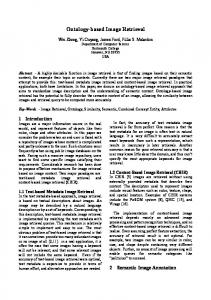
Sort the pair-wise distances among points in ascending order. Repeat connecting the two points with an edge according to the order until a connected graph is obtained.
2.
Form
the
(
affinity
Wij = exp − d 2 xi , x j
)
matrix
W
defined
by
2σ 2 if there is an edge linking
xi and x j . Let Wii = 0 . 3.
2. THE TRANSDUCTIVE LEARNING METHOD FOR IMAGE RETRIEVAL
Symmetrically normalize W by S = D −1/ 2WD −1/ 2 in which D is the diagonal matrix with ( i, i ) -element equal to the sum of the ith row of W.
Different from traditional methods, which measure perceptual similarity based on pair-wise distance, in MRBIR, we measure relevance between the query and database images by exploring the relationship of all the data points in the feature space. To achieve this goal, we resort to the manifold ranking algorithm proposed in [29, 30]. The algorithm is initially used to rank data points along their underlying manifold, which is revealed by the relationship among all the data points. Although such manifold structure might not exist for images belonging to the same semantic concept, the way in which the relationship among all the data points is investigated can be well applied to measuring the relevance between the query and database images. In this section, we will introduce this algorithm, followed by some analysis of its application in MRBIR.
4.
Iterate f ( t + 1) = α Sf ( t ) + (1 − α ) y until convergence, where α is a parameter in [ 0,1) .
5.
Let fi* denote the limit of the sequence
{ fi ( t )} .
Rank
*
each point xi according to its ranking scores fi (largest ranked first).
Figure 1. Manifold ranking algorithm
2.3 Analysis of the Algorithm Next we will analyze the algorithm with respect to its transductive nature. The theorem in [30] guarantees that the sequence { f ( t )} converges to
2.1 Notation
Given a set of points χ = { x1 , K, xq , xq +1 , K, xn } ⊂
m
f * = β (1 − α S ) y −1
,
the first q points are the queries which form the query set, and the rest are to be ranked according to their relevance to the queries. Let d : χ × χ → denote a metric on χ which assigns each pair of points xi and x j a distance d ( xi , x j ) , and f : χ →
(1)
where β = 1 − α . Although f * can be expressed in a closed form, for large scale problems, the iteration algorithm is preferable due to computational efficiency. Using Taylor expansion, we have
denote
−1
f * = (I −αS ) y
a ranking function which assigns to each point xi a ranking score f i . Finally, we define a vector y = [ y1 , K ,
1.
(
)
= I + α S + α 2S 2 + K y
yn ] , in which T
(2)
= y + α Sy + α S (α Sy ) + K
yi = 1 if xi is a query, and yi = 0 otherwise.
Here, we omit the constant coefficient β since it will not affect the ranking result. From the above equation, we can grasp the idea of manifold ranking from another point of view. f * can be regarded as the sum of a series of infinite terms. The first term is simply the vector y , the second term is to spread the ranking scores of the query points to their nearby points, the third term is to further spread the ranking scores, etc. Thus the effect of unlabeled data is gradually incorporated into the ranking score.
2.2 The Ranking Process The procedure of the algorithm in [29, 30] is listed in Figure 1. An intuitive description of this algorithm is: a weighted graph is first formed which takes each data point as a vertex; assign a positive ranking score to each query while zero to the remaining points; all the points then spread their scores to the nearby points via the weighted graph; the spread process is repeated until a global stable state is reached, and all the points except the query will have their own scores according to which they will be ranked. Note that self-reinforcement is avoided by setting the diagonal elements of the affinity matrix to 0. The propagation of ranking score reflects the relationship of all the data points, since in the feature space, distant points will have different ranking scores unless they belong to the same cluster consisting of many points that help to link the distant points, and nearby points will have similar ranking scores unless they belong to different clusters. In the context of image retrieval, there is only one query in the query set. The resultant ranking score of an unlabeled image is in
2.4 Formation of the Weighted Graph When applied in MRBIR, the first step of the algorithm in Figure 1 is modified as: calculate the K nearest neighbors for each point; connect two points with an edge if they are neighbors. The reason for this modification is to ensure enough connection for each point while preserving the sparse property of the weighted graph. Notice that in this way, the constructed graph is not necessarily connected and may consist of several separate clusters, which is different from the original algorithm. An inevitable consequence of a disconnected graph is that not all the images will end up with
11
a ranking score. However, since the images without ranking scores are not connected with the queries whether directly or indirectly, we can conclude with high confidence that those images are irrelevant ones. In the context of image retrieval where we pay much attention to the images ranked first, the order of images that come last in the ranking list is of minor concern, i.e. we do not care how the irrelevant images are arranged. So we simply put the images with no ranking score in the tail of the ranking list without harming the overall performance.
spread ranking scores independently, and assign large value to images belonging to their corresponding neighborhood. The ultimate ranking score is the sum of these individual scores.
3.2 RF with Positive and Negative Examples Due to the asymmetry between relevant and irrelevant images, they should be processed differently. For example, in Rocchio formula [15], the initial query is moved towards positive examples and away from negative examples by different degrees; in MEGA [7], positive examples are used to learn the target concept in k -CNF , while negative examples are used to learn a k -DNF that bounds the uncertain region; some researchers even come up with the idea of introducing different penalizing factors for positive and negative examples into the optimization problem of SVM [11]. A deeper reason for this asymmetry is that relevant images tend to form certain clusters in the feature space, while irrelevant images occupy the remaining feature space.
As stated in [1, 21], defining a suitable affinity matrix W is of key importance. A commonly used distance function d ( xi , x j ) is the
L 2 distance, which results in a Gaussian kernel for defining edge weights in W. However, based on the experimental results in [6, 12, 22], we can draw a conclusion that L1 distance can better approximate the perceptual difference between two images than other popular Minkowski distances when using either color or texture representation or both. Replacing L 2 distance with L1 distance, we use the Laplace kernel in MRBIR to define the edge weights in W, which can be written as follows:
(
)
m
k L xi , x j = ∏ l =1
(
1 exp − xil − x jl σ l 2σ l
)
To accommodate this asymmetry, in MRBIR, positive and negative examples spread their ranking scores differently. To speak concretely, we first define two vectors y + and y − . The element of the former one is set to 1 if the corresponding image is the query or a positive example; while the element of the latter one is set to -1 if the corresponding image is a negative example. All the other elements of the two vectors are set to 0. Secondly, let
(3)
where xil and x jl are the lth dimension of xi and x j respectively;
A = β ( I − α S ) , and define two matrices A+ and A− which are −1
m is the dimensionality of the feature space; and σ l is a positive parameter that reflects the scope of different dimensions. Thus
(
m
)
(
Wij = k L xi , x j = ∏ exp − xil − x jl σ l l =1
)
used to propagate the ranking scores of positive and negative examples, i.e., f + * = A+ y + , f −* = A− y − , where f + * and f −* are the ranking scores obtained from positive and negative examples respectively. The final ranking score can be written as f * = f + * + f −* . Generally speaking, positive examples should make more contribution to the final ranking score than negative examples. The reasons can be explained as follows: for an unlabeled image, the farther it lies from positive examples in the feature space, the less possible it is also a positive one. However, we do not have a similar conclusion for negative examples: if an unlabeled image lies far from negative examples, the possibility that it is a positive one is not necessary enhanced, since it may not get closer to positive examples either.
(4)
Here, we omit the coefficient 1 ( 2σ l ) , since its effect on the affinity matrix W will be counteracted in the normalization step S = D −1/ 2WD −1/ 2 and will not contribute to the final ranking result.
3. RELEVANCE FEEDBACK 3.1 RF with Only Positive Examples When only positive examples are available from the user’s feedback or when we consider only the relevant images, several schemes can be applied, making use of the information to improve retrieval accuracy. For example, the authors of [14] propose two query expansion approaches that selectively add relevant objects to the query, namely similar expansion and distant expansion; another approach adopted by [2] estimates the distribution of the target images in the feature space using one-class SVM. In this specific context, the manifold ranking algorithm can be easily generalized: add the newly obtained positive examples into the query set, and rerun the manifold ranking algorithm to refine the retrieval result. In this way, the vector y will have multiple nonzero components that will spread their ranking scores in the propagation process. And the sequence { f ( t )} converges to f * = β (I −αS ) y = β (I −αS ) −1
−1
Based on the above discussion, in MRBIR, we fix A+ , and explore the following three schemes for designing A− : In the first scheme, we set A− = γ A+ , which simply impair the contribution of the negative ranking score to f * by using a parameter γ ∈ ( 0,1] : the smaller γ is, the less impact negative examples will have on f * . When γ = 1 , there is no de-emphasis on negative examples. The second scheme is based on equation (2), i.e.,
(
M
≈ β ∑α i S i y −
+
n +1
∑y
i
(
)
f −* = β y − + α Sy − + α S α Sy − + K
)
(6)
i =0
(5)
where the negative score is approximated using only the first
i =1
i
where y is a n-dimensional vector with the ith component equal
M terms.
to 1 and others equal to 0, and n + is the number of positive examples fed back by the user. Therefore these examples will
M
Thus A− = β ∑ α i S i , this can be directly i =0
calculated without the iteration steps. In this scheme, the
12
ranking scores of negative examples only spread to nearby points, and their effect on distant points is negligible.
absolute value of f i −* indicates the irrelevance of an unlabeled image determined by negative examples, a small value of fi * = fi + * + fi − * means that the image is judged to be relevant by
In the third scheme, we modify the neighborhood of a negative example by changing σ l . Recall that σ l denotes a set of parameters introduced to calculate Wij .
the same degree as it is judged to be irrelevant, therefore, it can be considered an inconsistent one. From the perspective of information theory, such images are most informative.
It also
controls the neighborhood size within which the points will have a big similarity value to the center point: the bigger σ l is, the larger the neighborhood size. Therefore, we deliberately decrease σ l to obtain σ l′ , and calculate another
The third method tries to take the advantage of the above two schemes by selecting the inconsistent images which are also quite similar to the query. To speak concretely, we define a criterion function
similarity matrix W ′ for propagating negative ranking scores, using σ l′ . i.e. m
(
Wij′ = ∏ exp − xil − x jl σ l′ l =1
)
feedback. The criterion can be explained intuitively as follows: the selected images should not only provoke maximum disagreement among labeled examples (small fi +* + f i −* ), they
(7)
−1
σ l′ = η ⋅ σ l ( 0 < η < 1)
must also be relatively confidently judged as a relevant one by the positive examples (large f i + * ). We justify this scheme as follows: generally speaking, since positive examples occupy a small region in the feature space and are surrounded by negative examples, to identify the true boundary separating the two classes of images with a small number of labeled examples, it is more reasonable to explore in the inconsistent region near positive examples than in the entire inconsistent region. If an image is far from all the labeled examples, it will have a small value for both f i + * and
Thus the neighborhood of negative examples is smaller than that of positive examples, and the scope of their effect is decreased. In Section 6 we give experimental results to compare the three schemes, and incorporate the best one into MRBIR.
4. ACTIVE LEARNING METHODS Contrary to passive learning, in which the learner randomly selects some unlabeled images and asks the user to provide their labels, active learning selects images according to some principle, hoping to speed up the convergence to the query concept. This scheme has been proven to be effective in image retrieval by previous research work [25, 7]. In MRBIR, we develop three active learning methods based on different principles, which intentionally select images in each round of relevance feedback, aiming to maximally improve the ranking result. +*
+
+
(8)
Unlabeled images with the largest value of c ( xi ) are selected for
S ′ = D′−1/ 2W ′D′−1/ 2 A− = β ( I − α S ′ )
c ( xi ) = fi + * − f i + * + f i −*
−*
−
f i −* , and a small fi +* + f i −* accordingly, thus it is likely to be selected by the second scheme although it makes small contribution to the refinement of the boundary. However, it is not likely to be selected by the third scheme according to equation (8). Therefore, this scheme is expected to outperform the second one.
5. IMPLEMENTATION ISSUES One crucial element in designing an applicable CBIR system is the response time. It is unimaginable that the user has to wait a long time before the system is able to return satisfactory retrieval results. In the manifold ranking algorithm, we have to calculate the multiplication of large scale matrices in the iteration step. However, after the graph is simplified by connecting only neighboring points, we can use a sparse representation for matrices W and S, which are calculated off-line. In this way, the processing time can be greatly reduced. Another acceleration scheme is based on sampling techniques, which reduces the scale of the weighted graph to form a small graph, and propagates the scores of labeled images to its vertexes. For images not in the small graph, their scores can be obtained by exploring their neighborhood relationship with images in the small graph.
−
As pointed out in Section 3.2, f = A y and f = A y , which are the ranking scores obtained from positive and negative examples respectively. The final ranking score f * = f + * + f −* . For an unlabeled image xi , f i* is in proportion to the conditional probability that xi is a positive example given present labeled images: the larger f i* is, the bigger the probability. The first method is to select the unlabeled images with the largest f i* , i.e., the most relevant images, which is widely used in previous research work [4, 17, 18, 28]. The motivation behind this simple scheme is to ask the user to validate the judgment of the current system on image relevance. Since the images presented to the user are always the ones with the largest probabilities of being relevant, many of them might be labeled as positive, which will help the system refine the query concept; while the negative feedback images will help to eliminate false positive images.
Another issue is with respect to the query image. Recall that the weighted graph takes the query point as a vertex. If the query image is in the database, we can directly use the matrices W and S which are calculated off-line to rank the unlabeled images. On the other hand, if the query image is not in the database, we first project it to a point in the feature space. Next we connect the query with its K nearest neighbors in the image database, and calculate the edge weights by equation (4). Thirdly, we add one row and one column to W, with each element equal to the
The second method is to select the unlabeled images with the smallest f i* . Since the value of f i + * indicates the relevance of an unlabeled image determined by positive examples, while the
13
for Scheme 3. We have observed that to achieve satisfactory results, γ should lie within [0.1, 0.5]; M can be any integer between 2 and 5; and η should lie within [0.3, 0.7].
corresponding edge weight. All the other operations will be performed similarly using this enlarged matrix W.
6. EXPERIMENTAL RESULTS
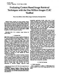
In Figure 3, we have compared the performance of the three schemes with the following parameter settings: γ = 0.25 ; M = 3 ; and η = 0.5 . Furthermore, we also present the result when γ = 1 in Scheme 1 (denoted as “Ref”). In this case, positive and negative examples are treated without difference. Obviously, the three schemes with proper parameter settings outperform this naive method, which validates the asymmetry between positive and negative examples discussed in subsection 3.2. For example, P10 using Scheme 1 is 0.540, using Scheme 2 is 0.531, using Scheme 3 is 0.520, and using “Ref” is 0.503. Moreover, Scheme 1 is slightly better than the other two despite of its simplicity. Therefore, Scheme 1 is incorporated into MRBIR.
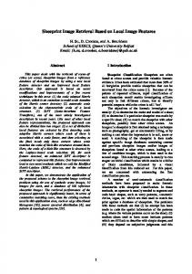
We have evaluated the performance of MRBIR using a generalpurpose image database consisting of 5,000 Corel images. The images are categorized into 50 groups, such as beach, bird, mountain, jewelry, sunset, etc. Each of the categories contains 100 images of essentially the same content, which serve as the groundtruth. We use each image in the whole database as a query, and average the results over the 5,000 queries. The precision vs. scope curve is used to evaluate the performance of various methods. Feature selection is a large open problem and might have a great impact on the results. In our current implementation, the feature vector is simply made up of color histogram [23] and wavelet feature [26] since we focus on the relative performance comparison1. Color histogram is obtained by quantizing the HSV color space into 64 bins. To calculate the wavelet feature, we first perform 3-level Daubechies wavelet transform to the image, and then calculate the first and second order moments of the coefficients in High/High, High/Low and Low/High bands at each level. We will leave the problem of selecting the optimal feature combination to future work.
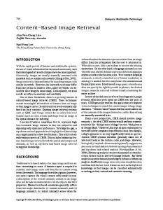
L2 distance
MRBIR(Laplace kernel)
MRBIR(Gaussian kernel)
0.35
Precision
0.3
There are four parameters needed to be set in the manifold ranking algorithm: K, α , σ l and the iteration steps. The algorithm is not very sensitive to the number of neighbors. In our experiments, we set K = 200 . α is fixed at 0.99, consistent with the experiments performed in [29, 30]. The value of σ l is problem-dependent. A
0.25 0.2 0.15 0.1 10
20
30
40
50
60
70
80
90
100
Scope
Figure 2. Comparison without relevance feedback.
principled way for determining σ l is setting it to be the average value in the lth dimension. In our current implementation, we set it to be 0.05 for all dimensions for the sake of simplicity. The number of iteration steps is 50, since we observe no improvement in performance with more iteration.
Scheme 1 Scheme 3
Scheme 2 Ref
0.55 0.5
Precision
0.45
6.1 MRBIR without Relevance Feedback As a new scheme of measuring similarity between images in CBIR, MRBIR is first compared with traditional methods based on pairwise distance when no relevance feedback is performed. The comparison results are illustrated in Figure 2. From the figure, we can see that MRBIR using Laplace kernel outperforms all the other methods, which confirms the method from two aspects: (1) by considering the relationship among all the data points, our method can better approximate relevance between the query and database images than traditional methods; (2) Laplace kernel is more suitable for defining edge weights than Gaussian kernel.
0.4 0.35 0.3 0.25 0.2 0.15 10
20
30
40
50
60
70
80
90
100
Scope
Figure 3. Comparison of the three schemes.
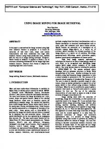
6.3 Relevance Feedback When both positive and negative examples are provided by the user, we apply MRBIR (with three active learning methods), SVM [28] and SVMactive [25] to refine the retrieval result, and compare their performance. For SVM and SVMactive, L1 distance is utilized in the initial retrieval stage and the adopted kernel is Gaussian kernel. To provide a systematic evaluation, we fix the total number of images that are marked by the user to 20, but vary the times of feedback and the number of images fed back each time accordingly. The combinations used in this experiment include: 1 feedback with 20 images each time; 2 feedbacks with 10 images each time; and 4 feedbacks with 5 images each time. In all the experiments, no matter which active learning method is taken, MRBIR outperforms SVM and SVMactive. In this section, we only present the results after the first and second rounds of
6.2 Comparison of Schemes for Incorporating Negative Examples As discussed in Section 3.2, we have three candidate schemes for designing A− . In order to select the best one to integrate into MRBIR, we have performed parametric study for each scheme: 0 < γ ≤ 1 for Scheme 1; 1 ≤ M ≤ 10 for Scheme 2; and 0 < η < 1
1
L1 distance
We have performed experiments with various features, such as color coherence, color correlogram, etc, and have reached the same conclusion.
14
relevance feedback with 5 images fed back each time, as in Figure 4.
in Table 1 (Pentium 4 1.80GHz, 512M RAM). Although MRBIR needs the longest time among all algorithms, it is still acceptable for both the search session and the feedback session.
In the first round of relevance feedback, the active learning part of both MRBIR and SVMactive is not provoked, and the most relevant images are labeled by the user. We did not adopt the scheme presented in [25], which asks the user to label randomly selected images in the first round of relevance feedback, since in this scheme, the information about the query is not utilized in the initial stage, which will inevitably result in slow convergence to the query concept.
Table 1. Comparison of Processing Time Time(second)
MRBIR
L1
SVM
SVMactive
Search
0.859
0.015
Feedback
0.859
0.062
0.062
MRBIR
SVM
0.5
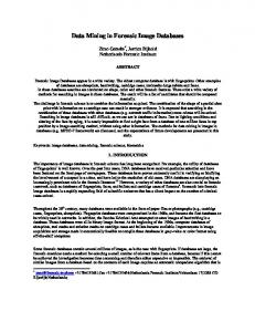
After the first round of relevance feedback (Figure 4(a)), MRBIR exhibits significant improvement over SVM. Take P10 (the precision within the first 10 retrieved images) as an example, for SVM, P10 is 0.260; while for MRBIR, it is 0.401, which exceeds SVM by about 54%. Similarly, P100 is 0.111 using SVM, and is 0.189 using MRBIR. The latter exceeds the former by about 70%. The reason lies in the fact that very few training examples may cause the decision boundary in SVM to distort greatly from the ideal one, while MRBIR can always relatively accurately predict the relevance of unlabeled images in the neighborhood of labeled examples.
Precision
0.4 0.3 0.2
0.1 0 10
20
30
40
50
60
70
80
90
100
Scope
(a)
When the second round of relevance feedback has been performed (Figure 4(b)), no matter which active learning method is taken, MRBIR outperforms SVM and SVMactive. Again we take P10 to demonstrate the advantage of MRBIR. For SVM, P10 is 0.265; for SVMactive, P10 is 0.239; while for the three active learning methods used in MRBIR, P10 is 0.478, 0.411, and 0.459 respectively. The best result obtained by MRBIR exceeds SVM by 80%, and SVMactive by 100%.
MRBIR1
MRBIR2
SVM
Active SVM
MRBIR3
0.6 0.5
Precision
0.4 0.3 0.2
Notice that comparing Figure 2 and Figure 4, SVM and SVMactive cause degradation in performance. Only after the system has accumulated enough labeled examples, are they able to refine the retrieval result; while MRBIR consistently increases the precision and outperforms SVM and SVMactive. Comparing Figure 4(a) and Figure 4(b), the improvement in P10 using SVM is only 0.005, while the improvement of MRBIR using the first active learning method is 0.077.
0.1 0 10
20
30
40
50 60 Scope
70
80
90
100
(b)
Figure 4. (a) Comparison after the first round of relevance feedback with 5 feedback images; (b) Comparison after the second round of relevance feedback (MRBIR1-MRBIR3 denote the three active learning methods).
Comparing the three active learning methods (Figure 4(b)), the performance of the second one (MRBIR2) is the worst, which selects the most informative images. The reason may be the lack of positive examples. When we try to capture a query concept with a limited number of labeled images, positive examples tend to be more important than negative ones. Since the second scheme selects the images which arouse the most disagreement among labeled images, the positive examples fed back in each round of relevance feedback is generally smaller than the other two methods, thus its performance is compromised. Of the remaining two methods, the first method is slightly better than the third one, which may lead to the following conclusion: in image retrieval where the labeled examples are quite limited, selecting the most relevant images in each round of relevance feedback may be the best strategy for active learning.
7. CONCLUSION In this paper, we propose a novel transductive learning framework named manifold-ranking based image retrieval (MRBIR), which is inspired by a recently developed manifold-ranking algorithm [29, 30]. The algorithm is initially proposed to rank data along their underlying manifold. In MRBIR, we use this algorithm to explore the relationship among all the data points in the feature space, and measure relevance between the query and database images, thus it addresses the limitation of present similarity metrics based on pair-wise distance. MRBIR also enables the user to perform relevance feedback, and provides different schemes to refine the retrieval result in case of the two types of feedback. Furthermore, we incorporate three active learning methods into MRBIR to speed up the convergence to the query concept. The methods make use of different principles to select images in each round of relevance feedback and ask the user for their labels. Experiments on a general-purpose image database consisting of 5,000 Corel images demonstrate that MRBIR outperforms existing methods.
In our experiments, MRBIR also greatly outperforms MARS [17, 18] when only positive examples are fed back by the user. Due to the limited space, we will not present specific results.
6.4 Processing Time We also compare the average response time of MRBIR using the first active learning method with existing systems, which is listed
15
MARS. Proc. IEEE Int. Conf. on Multimedia Computing and Systems, vol. 2, pp. 747-751, 1999.
8. ACKNOWLEDGEMENTS We would like to thank Shuicheng Yan, Xin Zheng, Lei Zhang and Xing Yi for their valuable discussions and enlightening comments. This work was supported by National High Technology Research and Development Program of China (863 Program) under contract No.2001AA114190.
[15] Rocchio, J.J. Relevance feedback in information retrieval. The SMART Retrieval System, pp. 313-323, Prentice-Hall, Englewood Cliffs, NJ, 1971. [16] Rubner, Y., Tomasi, C., and Guibas, L. A metric for distributions with applications to image databases. Proc. IEEE Int. Conf. on Computer Vision, pp. 59-66, 1998.
9. REFERENCES [1]
Bengio, Y., Vincent, P., and Paiement, J. Learning Eigenfunctions of Similarity: Linking Spectral Clustering and Kernel PCA. Technical Report 1232, University of Montreal, 2003.
[2]
Chen, Y., Zhou, X., and Huang, T. One-class SVM for learning in image retrieval. Proc. IEEE Int. Conf. on Image Processing, vol. 1, pp. 34-37, 2001.
[3]
Huang, J., et al. Image indexing using color correlograms. Proc. IEEE Conf. on Computer Vision and Pattern Recognition, pp. 762-768, 1997.
[4]
Jing, F., et al. An effective region-based image retrieval framework. Proc. 10th ACM Int. Conf. on Multimedia, 2002.
[5]
Ishikawa, Y., Subramanya, R., and Faloutsos, C. MindReader: querying databases through multiple examples. Proc. 24th Int. Conf. on Very Large Data Bases, 1998.
[6]
Kokare, M., Chatterji, B.N., and Biswas, P.K. Comparison of similarity metrics for texture image retrieval. IEEE Conf. on Convergent Technologies for Asia-Pacific Region, vol. 2, pp. 571-575, 2003.
[7]
Li, B., Chang, E., and Li, C.S. Learning image query concepts via intelligent sampling. Proc. IEEE Int. Conf. on Multimedia & Expo, pp. 961-964, 2001.
[8]
[9]
[17] Rui, Y., et al. Relevance feedback: a power tool for interactive content-based image retrieval. IEEE Trans. Circuits and Systems for Video Technology, 1998. [18] Rui, Y., Huang, T., and Mehrotra, S. Content-based image retrieval with relevance feedback in MARS. Proc. IEEE Int. Conf. on Image Processing, pp. 815-818, 1997. [19] Schmid, C. A structured probabilistic model for recognition. Proc. IEEE Conf. on Computer Vision and Pattern Recognition, vol. 2, pp. 490, 1999. [20] Schmid, C., and Mohr, R. Local grayvalue invariants for image retrieval. IEEE Trans. on Pattern Analysis and Machine Intelligence, vol. 19, pp. 530-535, 1997. [21] Shi, J., and Malik, J. Normalized cuts and image segmentation. IEEE Trans. on Pattern Analysis and Machine Intelligence, vol. 22, pp. 888-905, 2000. [22] Stricker, M., and Orengo, M. Similarity of color images. Storage and Retrieval for Image and Video Databases, Proc. SPIE 2420, pp 381-392, 1995. [23] Swain, M., and Ballard, D. Color indexing. Int. Journal of Computer Vision, 7(1): 11-32, 1991. [24] Tieu, K., and Viola, P. Boosting image retrieval. Proc. IEEE Conf. on Computer Vision and Pattern Recognition, vol. 1, pp. 228-235, 2000.
Li, B., Chang, E., and Wu, C.T. DPF-a perceptual distance function for image retrieval. Proc. IEEE Int. Conf. on Image Processing, vol. 2, pp. 597-600, 2002.
[25] Tong, S. and Chang, E. Support vector machine active learning for image retrieval. Proc. 9th ACM Int. Conf. on Multimedia, 2001.
Liu, F., and Picard, R.W. Periodicity, directionality, and randomness: Wold features for image modeling and retrieval. IEEE Trans. on Pattern Analysis and Machine Intelligence, vol. 8, 1996.
[26] Wang, J.Z., Wiederhold, G., Firschein, O., and Sha, X.W. Content-based image indexing and searching using Daubechies’ wavelets. Int. Journal of Digital Libraries, vol. 1, no. 4, pp. 311-328, 1998.
[10] Manjunath, B.S., and Ma, W.Y. Texture features for browsing and retrieval of image data. IEEE Trans. on Pattern Analysis and Machine Intelligence, vol. 18, pp. 837842, 1996.
[27] Wu, Y., Tian, Q., and Huang, T. Discriminant-EM algorithm with application to image retrieval. Proc. IEEE Conf. on Computer Vision and Pattern Recognition, vol. 1, pp. 155162, 2000.
[11] Morik, K., Brockhausen, P., and Joachims, T. Combining statistical learning with a knowledge-based approach––a case study in intensive care monitoring. Proc. 16th Int. Conf. on Machine Learning, 1999.
[28] Zhang, L., Lin, F., and Zhang, B. Support vector machine learning for image retrieval. Proc. IEEE Int. Conf. on Image Processing, vol. 2, pp. 721-724, 2001.
[12] Pass, G. Comparing images using color coherence vectors. Proc. 4th ACM Int. Conf. on Multimedia, pp. 65-73, 1997.
[29] Zhou, D., et al. Learning with local and global consistency. NIPS, 2003.
[13] Porkaew, K., and Chakrabarti, K. Query refinement for multimedia similarity retrieval in MARS. Proc. 7th ACM Int. Conf. on Multimedia, pp. 235-238, 1999.
[30] Zhou, D., et al. Ranking on data manifolds. NIPS, 2003. [31] Zhou, X.S., Rui, Y., and Huang, T. Water-Filling: a novel way for image structural feature extraction. Proc. IEEE Int. Conf. on Image Processing, vol. 2, pp. 570-574, 1999.
[14] Porkaew, K., Ortega, M., and Mehrota, S. Query reformulation for content based multimedia retrieval in
16