Accepted Manuscript
Manipulating higher dimensional spatial information Ken Arroyo Ohori ∗ Section GIS Technology, Delft University of Technology, The Netherlands
Filip Biljecki Section GIS Technology, Delft University of Technology, The Netherlands
Jantien Stoter Section GIS Technology, Delft University of Technology, The Netherlands Kadaster, Product and Process Innovation, Apeldoorn, The Netherlands Geonovum, Amersfoort, The Netherlands
Hugo Ledoux Section GIS Technology, Delft University of Technology, The Netherlands
ORCID KAO: FB: JS: HL: ∗
http://orcid.org/0000-0002-9863-0152 http://orcid.org/0000-0002-6229-7749 http://orcid.org/0000-0002-1393-7279 http://orcid.org/0000-0002-1251-8654
Corresponding author at
[email protected]
This is an Accepted Manuscript of an article published in the Proceedings of 16th AGILE Conference on Geographic Information Science held in Leuven, Belgium in May 2013, available online: http://doi.org/10.4233/uuid:c4751ad5-e008-48a6-806b-af38099e0b3a Cite as: Arroyo Ohori, K., Biljecki, F., Stoter, J., Ledoux, H. (2013): Manipulating higher dimensional spatial information. Proceedings of the 16th AGILE Conference on Geographic Information Science. Vandenbroucke, D. et al. (eds.). May 2013, Leuven, Belgium, pp. 1-7.
Abstract Real-world phenomena have traditionally been modelled in a GIS in two and three dimensions. However, powerful insights can be gained by the integration of additional non-spatial dimensions, such as time and scale, in a higher dimensional spatial model. While this theory is conceptually sound, there is a lack of understanding of its consequences when applied to real world geographic information. In this paper we therefore analyse these consequences, as well as the techniques that are necessary in order to extract meaningful 2D/3D information from it, which can be used with existing algorithms and software. Keywords: nD GIS; slicing; intersection; scale; time
1 Introduction There is substantial interest in the use of higher-dimensional (≥4D) digital objects that are built from real-world data. Within GIS, such objects can be produced when existing 2D/3D data is integrated with temporal information (Tøssebro and Nygård, 2011) or scale (van Oosterom and Meijers, 2012), among others. If these characteristics are considered as fully independent spatial dimensions (axes), objects in higher dimensional space are created. This powerful technique, explained fully in Section 2, is more complex than other representations (Peuquet and Duan, 1995; Claramunt et al., 1999; van Oosterom, 2005), but it is easily extensible to integrate other dimensions, and preserves all topological relationships within and between objects down to the vertex level. Doing so makes it possible to store continuously changing objects in time and scale, as well as other complex object relationships, and at the same time reduces redundancy and helps to avoid inconsistencies (van Oosterom and Meijers, 2012). Conceptually, these objects are hypervolumes of arbitrary shape. They can be closed (bounded) or open (unbounded), connected or not, with flat or curving boundaries, with or without holes, of equal or different dimension than the space they are contained in, orientable or unorientable, etc. However, in practical terms we are mostly interested in relatively simple orientable objects with flat geometry (polytopes), possibly with holes and possibly open (to support objects extending to infinity e.g. in time), in Euclidean space of the same or higher dimension than the objects. This is but an extension to higher dimensions of the typical objects currently found in 2D/3D GIS. We have therefore limited our scope to this class of objects, and within this paper, we will therefore only be concerned with them. Since it is difficult to visualise and analyse objects in more than three dimensions, we are also interested in extracting 2D or 3D objects from a higher dimensional representation. This is easily done at a conceptual level by computing the intersection of two sets of objects. However, computing these intersections for the general case is extremely difficult and computationally expensive. In fact, to the best of our knowledge, there is no software that is able to compute the intersection
1
of two arbitrary polytopes in more than three dimensions. We have therefore defined a simplified ‘slicing’ operation for this purpose—a limited form of point set intersection—which could realistically be implemented, and is covered in detail in Section 3. The goal of this paper is to establish a foundation for handling n-dimensional (nD) spatial information in a GIS context: a description of the nD geometries involved and how to reduce its dimensionality to 2D/3D. For this, we describe the necessary concepts, terms and definitions, both those common in 2D/3D GIS, and those derived from geometric modelling and mathematics (especially topology), and present their significance in the frame of reference of higher dimensional GIS. We finalise by showing some examples in Section 4, and our conclusions and plans for future work in Section 5.
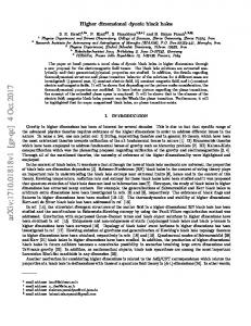
2 Higher dimensional spatial models To understand what we mean by considering all characteristics as independent (orthogonal) dimensions, let us first consider a case with 2D space, and time as the third dimension. At any one point in time, an object would be represented as a polygon in 3D space, parallel to the 2D space plane (x, y) and orthogonal to the time axis. Every object existing (and not moving or changing shape) during a time period would then be prism shaped, with identical base and top facets parallel to the 2D space plane and the other facets orthogonal to it. An example of this situation is shown in Figure 1. Extending this to a 4D representation of 3D space and time, every 3D object at one point in time would be a (3D) polyhedron in 4D space, and an object that exists for a period of time would be a polychoron, i.e. the four-dimensional analogue of a polygon/polyhedron. If this object is not moving or changing shape, it would take the form of a prismatic polychoron, i.e. the fourdimensional analogue of a prism. Another relevant application is the integration of scale as a spatial dimension. This concept is introduced in (Meijers and van Oosterom, 2011) in the variable-scale geo-information technique, and it is shown in Figure 2. Such approach enables the generation of an infinite number of continuous levels of detail, and provides a more consistent structure. The integration of scale can extend this concept to higher dimensions, e.g. to 4D in 3D city modelling (Stoter et al., 2012a,b). An d-dimensional spatial model is thus defined by a set of spatial objects embedded in d-dimensional space. This notion has been extensively studied and is universally used in GIS for d ≤ 3, but its logical consequences in d ≥ 4 have not been sufficiently explored. In particular, the distinction between the dimension of a spatial object and that of the space it is embedded in is not widely used or known in the GIS domain*. Even worse, 4D is often used as a catchphrase for 3D + time modelling, regardless of whether time is actually treated as an additional spatial dimension or not, and generally without creating any 4D objects.
*See Gold (2005) for an exception
2
Figure 1: A 2D space (x, y) + time (vertical axis) view of the footprint of two separate buildings at time t0 , which were connected by a corridor (red) from time t1 to time t2 and then became disconnected again when the corridor was removed until time t3 . The moments in time are shown along the thick line representing the front right corner of the right building.
t3
t2
t1
t0
time
y x
To understand the difference between the dimension of a spatial object and that of the space it is embedded in, it is useful to consider the manner in which a topology-based approach is used in geometric modelling. In such an approach, two semi-independent models are used: • A combinatorial or topological model that describes the topological relationships between and within spatial objects. To do this, certain assumptions about the topology of the objects are made, e.g. homeomorphism of an n-dimensional cell (n-cell), representing the topology of an n-dimensional spatial object, to an n-dimensional ball. • An embedding or geometric model that describes how these objects are embedded into geometrically defined space. Analogously, assumptions about the geometry of the objects are made as well, e.g. a closed polytope having no self-intersections. For instance, a cube could be represented in a combinatorial model as a 3-cell in a cell complex, described by its boundary of six 2-cells, each of those with a boundary composed of four 1-cells, each of them with a boundary composed of two 0-cells. A corresponding simple embedding model could relate each vertex (0-cell) to a tuple of coordinates and assume a linear geometry. More complex embedding models could contain explicit equations of curves, surfaces, etc. The distinction between the combinatorial and embedding models is useful from a scientific perspective since it separates the problems of the fields of geometric modelling and computational geometry (Lienhardt, 1994). When creating higher dimensional spatial models, the dimension
3
Figure 2: A 3D representation of 2D space (horizontal plane) and scale (vertical axis). The vertical edges connecting corresponding features have been omitted for legibility reasons. Adapted from Meijers and van Oosterom (2011).
4
of the spatial objects is given by the combinatorial model used, while the dimension of the space is given by its embedding model. Using this distinction, subtle differences can be recognised between different data models. For instance, both the winged-edge (Baumgart, 1975) and the facet-edge (Dobkin and Laszlo, 1987) data structures can be used to describe three dimensional models (sets of objects embedded in three dimensional space), but while the former is actually a 2D data model representing the (2D) manifold surface of the 3D objects within the model, the latter is a 3D data model fully capable of storing more complex objects and volume-volume relationships. Since different combinatorial models are usually able to represent mathematically different classes of objects, giving a precise definition of the dimension of a combinatorial model is complex and out of the scope of this paper. For the purposes of this discussion, we will therefore simplify it by assuming that an n-dimensional model is able to store every possible spatial object of dimension n. The dimension of a spatial object a, dim(a) ∈ N, is then given by the minimum dimension of a combinatorial model that is able to store it. Meanwhile, the dimension of a set of spatial objects A = {a0 , a1 , . . . , an } is given by the minimum dimension of a combinatorial model that is able to store all of these objects and the topological relationships between them, and is thus given by dim(A) = max(dim(a0 ), dim(a1 ), . . . , dim(an )) + adj, where adj = 1 if any two spatial objects of the highest dimension in the model are adjacent†, adj = 0 otherwise. Since this might be difficult or expensive to compute, one can safely assume dim(A) ≤ max(dim(a0 ), dim(a1 ), . . . , dim(an ))+ 1 instead. This reinforces the intuitive notion of the dimension of a set of isolated points being zero, line segments one, polygons two, polyhedra three, and so on, regardless of the dimension of the space they are embedded in. At the same time, this definition also clarifies dubious cases, such as a polyline being of dimension two or a planar partition of dimension three, not surprising considering that a (non self-intersecting) polyline is akin to an open polygon, or a planar partition an open polyhedron. Note however that this also entails that a single line segment implicitly described by its endpoints can have dimension zero, a polygon one, a polyhedron two, and so on. A single point cannot be implicitly described by its (null) boundary, and thus still has dimension zero. Meanwhile, the dimension of a space S in which the objects are embedded is also dim(S ) ∈ N, and is given by the dimension of the embedding model used. In a strict sense, the dimension of this model can be defined in terms of the dimension of the vector space defined in it. In the most common case, where it consists of a tuple of coordinates in a coordinate system whose axes are linearly independent, the dimension of the embedding model is the simply given by the number of coordinates used. Thus, when Rd is used‡, in practice it means that dim(Rd ) = d. It is worth noting that the dimensions of the objects and the space are independent of each other. As mentioned previously, topological models of one dimension lower than their corresponding geometry can be used, generally by representing an object implicitly by its boundaries. This saves †Adjacency between n-dimensional objects being defined as (n − 1)-adjacent. ‡Conceptually Rd is often used, but due to limitations inherent in computer representations, most likely something else is used when it is actually implemented (Goldberg, 1991).
5
on memory when the highest dimensional topological relationships are not required. On the other hand, it is also possible to have topological models of higher dimension than their actual geometric embedding, such as when 3D models are displayed on screen (or on paper), and are thus given a 2D geometry. However, this imposes considerable constraints, such as not being able to visualise the higher dimensional primitives, e.g. when drawing a 3D object in a 2D perspective view in a piece of paper, not all of its facets can be seen at the same time. For most GIS applications the dimension of the space is thus higher or equal to that of the objects within it.
3 Reducing the dimension of spatial objects Starting from a higher dimensional spatial model where a set of higher dimensional spatial objects are stored, being able to extract meaningful 2D/3D objects is a valuable operation. These simpler types are both easier to visualise and are possible to use with existing algorithms and software. In order to reduce the dimension of spatial objects, (point set) intersections of the original data in the model and purposefully designed lower dimensional objects can be used. This procedure works in a analogous manner as the generation of 2D cross-sections from 3D objects, such as is commonly done with isolines from elevation data. In the most general form, any two sets of objects A, B can be intersected (∩), resulting in a new set of objects A ∩ B, such that dim(A ∩ B ) ≤ min(dim(A), dim(B )). Since the intersection result is, by definition, the common part of the two sets of objects, it cannot be of a higher dimension than the lower dimensional set. In fact, it can be of a lower dimension than both, since they can touch at a lower dimensional primitive, e.g. a common point edge, or polygon. When the objects are disjoint, A∩B is empty (∅) and its dimension is not well defined, although 0 (Munkres, 1975) and −1 (Engelking, 1977) can be arguably justified mathematically, based on different definitions of the topological dimension of a set. Note however that even in the case of the intersection of two single objects, the result might not be a single object, i.e. single polytopes are not closed under the intersection operator. This is the reason why for our purpose, intersection is best treated directly based on sets of objects. Computing the intersection of two arbitrary sets of objects is a very complex problem. This can be somewhat ameliorated by restricting the objects that are allowed, such as for the convex case (Grünbaum, 1967); or by using techniques to subdivide the objects into more manageable ones, such as constrained triangulations (Shewchuk, 2000) or the alternate hierarchical decomposition (Bulbul and Frank, 2009). However, these techniques fail to fully overcome what is still an intricate problem with a very high computational complexity. Even in the convex case, it is likely analogous to the problem of computing an arrangement of hyperplanes, which is O(nd−1 ) in the worst case (Edelsbrunner et al., 1993), with n the total number of faces ((d − 1)-cells) in the two objects together. Since we are mostly interested in very specific cases of intersections, this problem can be often avoided by using the properties of the particular objects that need to be intersected. For this, we have defined the ‘slicing’ operator. Slicing is an intersection where a higher dimensional set of objects, generally consisting of a spatially indexed and rather large data set, is intersected with
6
another lower-dimensional object—often half-open, box-shaped and parallel to an axis—which we have dubbed as the ‘slicing element’. The end result is then often given in terms of the lower dimensional space induced by the slicing element itself, which is equivalent to an orthographic projection of the intersection to a coordinate system describing the vector space where the slicing element lies. An example of slicing is shown in Figure 3. Figure 3: Slicing a prism with a plane in 3D space. The data set object (blue prism) is sliced with the plane x3 = c (green slicing element), which is an open range along both x1 and x2 , and orthogonal to the axis x3 . The resulting object (red) is a triangle in 3D space. This triangle can also be expressed as a triangle in the 2D space x1 ×x2 induced by the slicing element. x3 = c
B
x1
x2
A
\
x1
A
B
A\B
x3 = c
A c
x3
x3
x2 B
This operation can be expressed as follows. Given a data set object A ∈ x1 × x2 × x3 , where dim(A) = 3 and a specific value c of x3 along which we want to slice it, it is possible to generate the slicing element B ∶ x3 = c, where dim(B ) = 2. The result is given by A ∩ B ∈ x1 × x2 × x3 , where dim(A ∩ B ) = min(dim(A),dim(B )) = 2, and it can be expressed as a two dimensional object in the space x1 × x2 induced by the slicing element B.
4 Example Consider now what would happen in a practical example using a four dimensional model with 3D space and scale (level of detail), as shown in Figure 4. The model consists of a single 4D object representing a house at different levels of detail along the scale axis (l). Every d-dimensional primitive in the house is thus a (d + 1)-dimensional one in the model, stretching from the minimum level of detail where it is visible up to the maximum level of detail, its geometry becoming increasingly complex and joined appropriately. For instance, the vertex at the apex in the front of the house is a (poly)line connecting the apices at different scale levels. Similarly, the edge between the roof of the house and its façade is a (set of adjacent) planes joining these edges at different scales. For this paper we ignore how these are joined, but work is ongoing to achieve this purpose. An alternative view is considering that a 3D object at a fine level of detail (l3 ) has been generalised (using generalisation algorithms) in several steps up to a coarse level of detail (l1 ), and these have been joined appropriately. By slicing this space-scale 4D object, it is possible to generate 3D models at intermediate levels of detail, such as the house at an arbitrary value, e.g. l = l2 .
7
Figure 4: A schematic view showing the results of slicing a 4D model consisting of 3D space (x, y, z) and 1D scale l (red axis). The model contains a house at levels of detail ranging from coarse (l1 ) to fine (l3 ) An intermediate level of detail can be obtained from the model by slicing it at the scale value of l = l2 and projecting it to the hyperplane of the slicing element.
z y x l1
l2
l3
l
Unlike other models with fixed representation levels, there are an infinite number of differently detailed 3D models that can be extracted from this 4D one, allowing for smooth zooming operations (van Oosterom and Meijers, 2012) or obtaining levels of detail that are optimised for the screen in which they are viewed.
5 Discussion The simple example from the previous section does not show all the advanced capabilities that can be achieved using a true 4D spatial model. For instance, using a slicing element with linear geometries, but that is not orthogonal to the scale axis, it is possible to obtain mixed-scale levels of detail for applications where different levels of detail across the view are required, e.g. having more detail close to the viewer or in an area where a detailed simulation is needed (perspective view). Slicing with multiple disjoint planes (a discontinuous embedding) can generate views of the same object at different levels of detail or points in time. Animations can be generated by moving the slicing element along a meaningful path. Advanced representation can be obtained using curving objects, such as bell shaped surfaces for mixed scale that depends on the distance to the viewer. These possibilities are currently difficult to visualise, but we believe their implementation to be within reach, and the capabilities offered by true higher dimensional models open new and concrete possibilities for analysis. Having access to the full topological information means that the
8
connectivity between in within objects is never lost, e.g. an object disappearing and then reappearing in time, which allows for topological queries along all dimensions and avoids expensive computations to determine whether two objects are actually the same. For these reasons, the concepts presented in this paper are important as a foundation for the manipulation of higher dimensional spatial information.
Acknowledgements We thank the reviewers for their constructive comments. This research is supported by the Dutch Technology Foundation STW, which is part of the Netherlands Organisation for Scientific Research (NWO), and which is partly funded by the Ministry of Economic Affairs (project code: 11300).
References B. G. Baumgart. A polyhedron representation for computer vision. In Proceedings of the May 19-22, 1975, National Computer Conference and Exposition, pages 589–596, 1975. R. Bulbul and A. U. Frank. AHD: The alternate simplicial decomposition of nonconvex polytopes (generalization of a convex polytope based spatial data model). In Proceedings of the 17th International Conference on Geoinformatics, pages 1–6, 2009. C. Claramunt, C. Parent, S. Spaccapietra, and M. Thériault. Database modelling for environmental and land use changes. In J. C. H. Stillwell, S. Geertman, and S. Openshaw, editors, Geographical Information and Planning, Advances in Spatial Science, chapter 10, pages 181–202. Springer Berlin / Heidelberg, 1999. D. P. Dobkin and M. J. Laszlo. Primitives for the manipulation of three-dimensional subdivisions. In Proceedings of the 3rd Annual Symposium on Computational Geometry, pages 86–99. ACM, 1987. H. Edelsbrunner, R. Seidel, and M. Sharir. On the zone theorem for hyperplane arrangements. SIAM Journal on Computing, 22(2):418–429, April 1993. R. Engelking. General Topology. Polish Scientific Publishers, 1977. C. M. Gold. Data structures for dynamic and multidimensional GIS. In Proceedings of the 4th ISPRS Workshop on Dynamic and Multi-dimensional GIS, pages 36–41, Pontypridd, Wales, UK, 2005. D. Goldberg. What every computer scientist should know about floating-point arithmetic. Computing Surveys, 23(1):5–48, March 1991. B. Grünbaum. Convex polytopes. John Wiley, 1967.
9
P. Lienhardt. N-dimensional generalized combinatorial maps and cellular quasi-manifolds. International Journal of Computational Geometry and Applications, 4(3):275–324, 1994. M. Meijers and P. van Oosterom. The space-scale cube: An integrated model for 2D polygonal areas and scale. In 28th Urban Data Management Symposium, volume 38, pages 95–102, 2011. J. R. Munkres. Topology: A First Course. Prentice-Hall, Inc., 1975. D. J. Peuquet and N. Duan. An event-based spatiotemporal data model (ESTDM) for temporal analysis of geographical data. International Journal of Geographical Information Science, 9(1): 7–24, 1995. J. R. Shewchuk. Sweep algorithms for constructing higher-dimensional constrained Delaunay triangulations. In Proceedings of the 16th Annual Symposium on Computational Geometry, pages 350–359, 2000. J. Stoter, H. Ledoux, M. Meijers, and K. Arroyo Ohori. Integrating scale and space in 3D city models. In Proceedings of the 7th International 3D GeoInfo Conference, May 2012a. J. Stoter, H. Ledoux, M. Meijers, K. Arroyo Ohori, and P. van Oosterom. 5D modeling - applications and advantages. In Proceedings of the Geospatial World Forum 2012, page 9, 2012b. E. Tøssebro and M. Nygård. Representing topological relationships for spatiotemporal objects. Geoinformatica, 15:633–661, 2011. P. van Oosterom. Variable-scale topological data structures suitable for progressive data transfer: The GAP-face tree and GAP-edge forest. Cartography and Geographic Information Science, 32 (4):331–346, 2005. P. van Oosterom and M. Meijers. Vario-scale data structures supporting smooth zoom and progressive transfer of 2D and 3D data. In F. Schröder, editor, Jaarverslag 2011, pages 21–42, Delft, the Netherlands, 2012. Nederlandse Commissie voor Geodesie - Netherlands Geodetic Commission. P. van Oosterom and M. Meijers. Vario-scale data structures supporting smooth zoom and progressive transfer of 2D and 3D data. In Jaarverslag 2011. Nederlandse Commissie voor Geodesie, 2012.
10