Many-mode Entanglement in Continuous-variable Systems - Applied ...

Many-mode Entanglement in Continuous-variable Systems

Helen Sarah McAneney, MSci

Thesis submitted for the degree of Doctor of Philosophy in the Faculty of Science and Agriculture Queen’s University, Belfast

December 2004

This work is dedicated to my loving husband Jonny, without whose support, determination and understanding I would never have reached this far.

“In physics, you don’t have to go around making trouble for yourself - nature does it for you.” Frank Wilczek

“It is often stated that of all the theories proposed in this century, the silliest is quantum theory. In fact, some say that the only thing that quantum theory has going for it is that it is unquestionably correct.” Michio Kaku

Acknowledgments I want to take this opportunity to thank those who have made my Ph.D. years very enjoyable ones, as well as those who have helped support and encourage me when I have needed it most. Firstly, thanks must go to my supervisor Dr. Myungshik Kim, for his never ending patience and guidance throughout my Ph.D. To Dr. Jinhyoung Lee, whose inspiration and vast knowledge gave rise to the concept of collective modes, as a consequence of the work of Chapter 4, and from this concept, the main work in Chapter 3 arose. Also to Mauro Paternostro, for his insight into how the decomposition provided in Chapter 5 could be applied to the distribution of entanglement. I am also grateful to Mauro for taking time out of his very busy schedule to not only read this thesis, but also for his criticisms and suggestions that have improved my writing greatly. Mauro’s passion and enthusiasm for science has been an inspiration to behold. The many others in our Quantum Optics group, past and present, I also thank. Everyday would not have been the same without sharing an office with Claire McKenna, and later with Sharon Gilmore and Liz O’Sullivan. To Claire I owe a sincerest amount of thanks for her true friendship and comradeship, not only through these postgraduate years, but also through our M.Sci. She has kept me sane and always listened to my raving on. Moreover, for the girls’ endless supply of chocolate cakes whenever it was anyone’s birthday, and the organisation of many group lunches. I must also thank the members of Jonny’s research group, who include Stephen Campbell and Alison McMullan, fellow Ph.D. students with whom I have spent many lunches and tea breaks discussing the most bizarre concepts with. For Alison’s optimism and good humour (even though she had to sit beside Jonny) and Stephen’s forever promise of a barbecue. They are both true friends without whom life would be very dull. Additionally, I must mention Dr. Marty Gregg and Dr. Robert Bowmen, who have treated me as one of the research group and given me both advice and encouragement. Within the Department of Applied Mathematics and Theoretical Physics, I am grateful for the support that Professor Alan Hibbert and Professor James Walters iii

have provided by always having time to listen or to have a chat. I am appreciative of being able to have worked alongside Dr. Gleb Gribakin, Dr. Jorge Kohanoff and Dr. Francesca O’Rourke by helping with teaching duties and to have come to know them. Additionally, I have greatly appreciated the time and effort that Andrew Gallagher always has had for me, in regard to computing needs and friendship. A word of gratitude must go to Professor Mike Finnis whose supervision and encouragement in my MSci project, and belief in my abilities has sparked an interest in research. His ability to make me question further, I fill never forget. To my family and friends, I am truly grateful for the never ending support and faith in by abilities. To my parents, I am very appreciative of their patience and understanding of the decisions I have made throughout the years, both good and bad, and for giving me the freedom to have made such choices. To the in-laws, a word of sincere thanks for always making me feel welcome. Last, but by no means least, I wish to thank my husband Jonny, who has been a source of continual support and encouragement in my years of study and research. For his patience in explaining the physics of many a problem, as well as our debates over the how and why. Without Jonny, I would never have conceived of doing a Ph.D., and so now I am immensely grateful that I have had the opportunity to have worked along side many amazing people, in an area of great intrigue.

iv

Abstract Techniques to study the entanglement within continuous variable systems have been developed in the last few years for simple configurations of one-mode vs another, or the entanglement between one-mode and many. However, less is known in regard to the entanglement structure of many-mode systems. This thesis is the study of such entanglement structures, both within the context of the loss of coherence and the distribution of entanglement. The decoherence process occurs due to the loss of information to the environment. The standard Born-Markov approximation for the derivation of the master equation does not allow any memory effects, and hence is only valid for the short term dynamics. A method is outlined here, in which the reduced dynamics of the system are completely positive and valid even in the long term. This method makes use of the collective approach, which allows for an alternative mathematical perspective of the problem, whilst the physics of the overall system is maintained. Although the correct dynamical behaviour can be obtained from the master equation by the Born-Markov approximations for the short time scale, in the collective approach no approximations are made. Both approaches describe the dynamical evolution of the same system, and hence are required to be the same in the short term, but the collective approach is also valid for the long term. A comparison of the two methods yields two conditions upon the dynamics achieved from the collective approach. The Markovian interaction can be modelled by an array of infinite beam-splitters with thermal input fields. This model is applied in three scenarios. Given an initial two-mode system, one of which is influenced by the environment model, whilst the other is isolated. The entanglement structure of the evolved total system was then calculated. A finite number of beam-splitter interactions were considered, and the results indicated the same outcome in the entanglement properties whether one, two, or one hundred environmental modes were considered, provided the transmittivity of each beam-splitter interaction is appropriately scaled so that one has the same total interaction time. This gave rise to the concept of the collective environment, with one collective mode interacting with the initial system. Results were found to be equivalent, i.e. by considering the v

environment as one group of modes (or one collective mode), tripartite entanglement is formulated, and depending on the interaction time and the temperature of the thermal field, either two, one or no forms of pairwise entanglement exists between two of the modes. Thus, at the time of the decoherence of the initial two-mode system, there are two paths by which this can occur. In the low temperature regime, the decoherence happens through two-way entanglement, but in the high temperature regime, GHZ entanglement was formed by the collective environment and the two system modes. The purity of the initial system was also calculated and found to take exactly half its maximum value at the point were these two paths of decoherence emerge. It is known that the tracing over of one-mode of a two-mode squeezed state creates a thermal state, and so the complete set-up of the model was studied, where symmetric results were obtained. Lastly, the study was extended with the inclusion of local squeezing on the two-modes of the initial system. Results indicated a similar entanglement structure for the total system, only with the inclusion of a third option of pairwise entanglement from the interacting modes. The two conditions for this third type of pairwise entanglement now depends on the local squeezing parameters as well as the transmittivity, temperature and two-mode squeezing parameter. Finally, a Hamiltonian capable of governing the evolution due to non-Markovian type interactions was studied. The evolution of the modes was calculated, and from this, the transformation required for the initial variance matrix to that of the evolved one was achieved. Thus, the entanglement properties, given any initial state, could be investigated. Additionally, the evolution operator was found to be decomposable into a combination of beam-splitters and rotators, such that the same evolution of the modes is achieved. This is valid in the case of resonant interactions. An application of this study has been applied to the distribution from one central root to a collection of others via this polyandry type interaction. Both the single excitation and continuous variable case were investigated, and both found to be efficient in the distribution of entanglement.

vi

Publications Peer Reviewed Journals • M. Paternostro, H. McAneney and M.S. Kim. “Multi-splitter interaction for entanglement distribution.” Phys. Rev. Lett. 94, 070501 (2005).

• H. McAneney, J. Lee, D. Ahn and M.S. Kim. “Non-Markovian Decoherence: Complete Positivity and Decomposition.” J. Mod. Opt. (2005). Accepted for publication.

• J. Lee, I. Kim, D. Ahn, H. McAneney and M.S. Kim. “Completely-Positive Non-Markovian Decoherence.” Phys. Rev. A 70, 024301 (2004).

• J. Lee, H. McAneney and M.S. Kim. “On the Disentangling Process for Two-Mode Squeezed State.” J. Korean Phys. Soc. 44, 691-696, Part 2 (March 2004).

• H. McAneney, J. Lee and M.S. Kim. “Many-body entanglement in decoherence processes.” Phys. Rev. A 68, 063814 (2003)

Other Publications • H. McAneney, J. Lee and M.S. Kim. “Entanglement of a Gaussian System with a Thermal Environment.” Proceedings of the 8th International Conference on Squeezed States and Uncertainty Relations, page 277-283 (Rinton Press, 2003). vii

Table of Contents

ACKNOWLEDGEMENTS

iii

ABSTRACT

v

PUBLICATIONS

vii

TABLE OF CONTENTS

viii

LIST OF FIGURES

xiii

LIST OF TABLES

xv

1 INTRODUCTION

1

1.1 Historical Viewpoint . . . . . . . . . . . . . . . . . . . . . . . . .

2

1.2 What is entanglement? . . . . . . . . . . . . . . . . . . . . . . . .

4

1.3 Why entanglement is studied

7

. . . . . . . . . . . . . . . . . . . .

1.4 Types of systems . . . . . . . . . . . . . . . . . . . . . . . . . . . 10 1.5 Motivation and Outline . . . . . . . . . . . . . . . . . . . . . . . . 12 2 BACKGROUND THEORY

15 viii

Table of Contents 2.1 Basic Concepts: Separable or Entangled? . . . . . . . . . . . . . . 16 2.2 CV Notation and Terminology . . . . . . . . . . . . . . . . . . . . 19 2.2.1

Operators and States . . . . . . . . . . . . . . . . . . . . . 19

2.2.2

The Characteristic Function . . . . . . . . . . . . . . . . . 25

2.2.3

Different Types of Entanglement . . . . . . . . . . . . . . 28

2.3 Entanglement Criteria I . . . . . . . . . . . . . . . . . . . . . . . 30 2.3.1

The Reduced Density Matrix . . . . . . . . . . . . . . . . 30

2.3.2

The Schmidt Decomposition . . . . . . . . . . . . . . . . . 32

2.3.3

Separability Criteria for Mixed States . . . . . . . . . . . . 33

2.4 Entanglement Criteria II . . . . . . . . . . . . . . . . . . . . . . . 34 2.4.1

Simon’s Criterion . . . . . . . . . . . . . . . . . . . . . . . 34

2.4.2

Bound Entangled States . . . . . . . . . . . . . . . . . . . 38

2.4.3

Giedke’s et al. Criterion . . . . . . . . . . . . . . . . . . . 40

2.5 Characterisation of Entanglement . . . . . . . . . . . . . . . . . . 44 2.5.1

Measures of Entanglement . . . . . . . . . . . . . . . . . . 45

2.5.2

Classification and Type . . . . . . . . . . . . . . . . . . . . 47

3 REDUCED DYNAMICS & DECOHERENCE

52

3.1 Decoherence . . . . . . . . . . . . . . . . . . . . . . . . . . . . . . 53 3.1.1

The Environment . . . . . . . . . . . . . . . . . . . . . . . 54

3.1.2

Reduced Dynamics of a System . . . . . . . . . . . . . . . 55

3.2 The Master Equation within the Born-Markov Approximation . . 56 ix

Table of Contents 3.2.1

Physical Derivation . . . . . . . . . . . . . . . . . . . . . . 57

3.2.2

Mathematical Derivation . . . . . . . . . . . . . . . . . . . 61

3.3 Complete Positivity of the Reduced Dynamics . . . . . . . . . . . 64 3.3.1

Complete Positivity . . . . . . . . . . . . . . . . . . . . . . 64

3.3.2

Collective Approach . . . . . . . . . . . . . . . . . . . . . 65

3.3.3

Methodology . . . . . . . . . . . . . . . . . . . . . . . . . 65

4 TOTAL SYSTEM DYNAMICS & DECOHERENCE

69

4.1 Model of the Markovian Environment . . . . . . . . . . . . . . . . 70 4.1.1

Physical Interpretation . . . . . . . . . . . . . . . . . . . . 72

4.1.2

N Environmental Modes . . . . . . . . . . . . . . . . . . . 73

4.1.3

One Collective Environmental Mode . . . . . . . . . . . . 75

4.2 Initial System of a Two-mode Squeezed State . . . . . . . . . . . 79 4.2.1

Correlations given a Finite Environment . . . . . . . . . . 81

4.2.2

Correlations given a Collective Environment . . . . . . . . 85

4.3 Results & Analysis . . . . . . . . . . . . . . . . . . . . . . . . . . 87 4.3.1

Equivalence of Two Approaches . . . . . . . . . . . . . . . 87

4.3.2

Multipartite Entanglement within Decoherence Process . . 88

4.3.3

Bound Entanglement? . . . . . . . . . . . . . . . . . . . . 91

4.3.4

Purity of the System . . . . . . . . . . . . . . . . . . . . . 102

4.4 The Complete Picture . . . . . . . . . . . . . . . . . . . . . . . . 103 4.5 General Non-Classical State . . . . . . . . . . . . . . . . . . . . . 105 x

Table of Contents 4.5.1

Results . . . . . . . . . . . . . . . . . . . . . . . . . . . . . 107

5 POLYANDRY INTERACTIONS

110

5.1 Polyandry Interactions . . . . . . . . . . . . . . . . . . . . . . . . 111 5.2 Evolution and Decomposition . . . . . . . . . . . . . . . . . . . . 114 5.2.1

The Evolution Operator . . . . . . . . . . . . . . . . . . . 114

5.2.2

Decomposition . . . . . . . . . . . . . . . . . . . . . . . . 117

5.3 Non-Markovian Type Interactions . . . . . . . . . . . . . . . . . . 119 5.3.1

Transformation . . . . . . . . . . . . . . . . . . . . . . . . 121

5.3.2

Remarks . . . . . . . . . . . . . . . . . . . . . . . . . . . . 122

5.4 Distribution of Entanglement . . . . . . . . . . . . . . . . . . . . 123 5.4.1

Entanglement Distribution: Single Excitation . . . . . . . 124

5.4.2

Entanglement Distribution: CV Case . . . . . . . . . . . . 128

5.4.3

Remarks . . . . . . . . . . . . . . . . . . . . . . . . . . . . 132

6 CONCLUSIONS

133

6.1 Conclusions . . . . . . . . . . . . . . . . . . . . . . . . . . . . . . 134 APPENDICES

140

A OPERATOR RELATIONS

140

A.1 Theorem 1 . . . . . . . . . . . . . . . . . . . . . . . . . . . . . . . 141 A.2 Theorem 2: The Baker-Campbell-Hausdorf Relation . . . . . . . . 142

xi

Table of Contents B SYMPLECTIC GROUPS

144

B.1 Properties of the Symplectic Group . . . . . . . . . . . . . . . . . 145 B.1.1 Real Symplectic Groups Sp(2n, R) . . . . . . . . . . . . . 145 B.1.2 Properties of Sp(2n, R) Matrices

. . . . . . . . . . . . . . 147

B.1.3 Variance Matrices . . . . . . . . . . . . . . . . . . . . . . . 148 B.2 Williamson’s Theorem & Uncertainty Principles . . . . . . . . . . 149 B.2.1 Single-mode Criterion & Squeezing . . . . . . . . . . . . . 150 B.3 Reasoning within Simon’s Criterion . . . . . . . . . . . . . . . . . 151 C NEGATIVITY AS A MEASURE OF ENTANGLEMENT

153

C.1 Negativity of Entanglement . . . . . . . . . . . . . . . . . . . . . 154 C.1.1 Bound Operator . . . . . . . . . . . . . . . . . . . . . . . . 154 C.1.2 Two-mode Gaussian Continuous Variable System . . . . . 155 C.1.3 Diagonalisation of V . . . . . . . . . . . . . . . . . . . . . 156 C.1.4 Positive Operator & the Uncertainty Principle . . . . . . . 157 C.1.5 Operator Equations . . . . . . . . . . . . . . . . . . . . . . 158 D COMPUTER PROGRAMS

162

D.1 Bi-separability of 1:1 Mode . . . . . . . . . . . . . . . . . . . . . . 163 D.2 Bi-separability of 1:2 Modes . . . . . . . . . . . . . . . . . . . . . 169 D.3 Bi-separability of 2:m Modes . . . . . . . . . . . . . . . . . . . . . 175 BIBLIOGRAPHY

183 xii

List of Figures

1. INTRODUCTION

2

1.1 Conceptual idea of superposition . . . . . . . . . . . . . . . . . .

5

1.2 Entanglement from a non-linear crystal . . . . . . . . . . . . . . .

6

1.3 Moore’s Law . . . . . . . . . . . . . . . . . . . . . . . . . . . . . .

8

1.4 The Bloch sphere . . . . . . . . . . . . . . . . . . . . . . . . . . . 11

2. BACKGROUND THEORY

16

2.1 Conceptual illustration of a pure or mixed state . . . . . . . . . . 18 2.2 Gallery of Quantum States I . . . . . . . . . . . . . . . . . . . . . 21 2.3 Gallery of Quantum States II . . . . . . . . . . . . . . . . . . . . 22 2.4 The Beam-Splitter . . . . . . . . . . . . . . . . . . . . . . . . . . 24 2.5 The Borromean Rings . . . . . . . . . . . . . . . . . . . . . . . . 29 2.6 Outline of Werner and Wolf’s reasoning for bound entangled states and NPT given 1 : N modes . . . . . . . . . . . . . . . . . . . . . 39 2.7 Entanglement summary for Gaussian bipartite systems . . . . . . 43

xiii

List of Figure 4. TOTAL SYSTEM DYNAMICS & DECOHERENCE

70

4.1 Infinite array of beam-splitters to model the Markovian environment 71 4.2 Finite array of beam-splitters to model the Markovian environment 74 4.3 One collective mode and beam-splitter to model the Markovian environment . . . . . . . . . . . . . . . . . . . . . . . . . . . . . . 76 4.4 Bipartite entanglement within the environment model . . . . . . . 84 4.5 A possible complete picture of the previous interactions . . . . . . 103 4.6 Bipartite entanglement for the complete picture . . . . . . . . . . 105

5. POLYANDRY INTERACTIONS

111

5.1 Schematic of Polyandry type interaction . . . . . . . . . . . . . . 112 5.2 Schematic of the decomposed evolution operator Eqn.(5.12) . . . . 118 5.3 Permutational invariant bipartite entanglement graph with respect to any pair of indexes . . . . . . . . . . . . . . . . . . . . . 124 5.4 Bipartite entanglement EN versus the number of elements N and the dimensionless coupling g . . . . . . . . . . . . . . . . . . . . . 129 5.5 Qualitative comparison of qubit and CV cases given the loss of pairwise entanglement with an increase in N for the distribution of entanglement . . . . . . . . . . . . . . . . . . . . . . . . . . . . 132

xiv

List of Tables

2. BACKGROUND THEORY

16

2.1 Variance matrices. . . . . . . . . . . . . . . . . . . . . . . . . . . 28 2.2 Classification of a three-mode Gaussian states. . . . . . . . . . . . 50

4. TOTAL SYSTEM DYNAMICS & DECOHERENCE

70

4.1 Equivalent determination of matrix nature from the determinants of the principal minors and eigenvalues. . . . . . . . . . . . . . . . 96 4.2 Illustration of positive semi-definite nature of the state . . . . . . 97 4.3 Demonstration of the non-positive semi-definite nature of the state after partial transposition of any single mode . . . . . . . . . . . . 98 4.4 Determination of pairwise entanglement conditions from the determinants of principal minor calculations . . . . . . . . . . . . . 99 4.5 Determinants of the principal minors given a 2:2 mode case. Bound entanglement is not present . . . . . . . . . . . . . . . . . . . . . 101

xv

Chapter 1

Introduction

1

1.1.

Historical Viewpoint “Perplexity is the beginning of knowledge.” Kahlil Gibran (1883-1931)

1.1

Historical Viewpoint

With the onset of quantum mechanics at the beginning of the last century, a new area of study emerged. Many today still struggle to come to terms and understand the bizarre concepts and ideas that it predicts. Nonetheless, time and again these quantum mechanical predictions have been proven experimentally correct. One of these bizarre concepts was termed “verschränkung” by Schrödinger in 1935 [1]. Literally translated it means “folding of arms”, however the rather loose translation of entanglement was introduced later the same year [2]. This latter meaning has since remained. From the 1920’s onwards, much debate over the true meaning and interpretation of quantum mechanics has taken place, in particular in the early days between Bohr and Einstein [3]. Within this debate a paper by Einstein, Podolsky and Rosen emerged in 1935, asking whether quantum mechanics was an incomplete theory [4]. Einstein referred to entanglement as “a spooky action at a distance”, and as such did not believe that “God would play dice”. Instead, his belief was that quantum mechanics was incomplete. This paper is now referred to as the EPR Paradox. In essence, it is stating how, under a certain setup, one can beat the Heisenberg uncertainty limit by knowing both position and momentum of a state at a given time. This is achieved by having two entangled bodies, and by the measurement of position on one, the position of the other is known. Similarly, if the momentum of the latter is measured then it is also known exactly for the former. Hence, the position and momentum of both bodies are known exactly. This is in clear violation of the uncertainty principle which states that there is a limit to the exact knowledge of conjugate pairs, such as position and momentum, of 4x4p > ~/2. Consequently, they concluded that quantum mechanics must be incomplete, rather than believe than entanglement existed. It must be noted, that although the measurement on one part of an entangled system alters the 2

1.1.

Historical Viewpoint

state of the other, the above paradoxical situation arises from the misuse of the measurement process with the action of simultaneous measurements. This paradoxical situation was resolved by John Bell in 1964 with the use of the theory of hidden variables [5, 6]. He assumed that some type of hidden variables existed which effected and controlled the behaviour of a state of two particles, and it was these variables that allowed the “spooky action at a distance” to occur. Given the existence of hidden variables, predictions were made, as was the case for quantum mechanics. These predictions came in the form of inequalities with an upper bound for the hidden variable theorem and a higher upper bound for quantum mechanics (Cirel’son’s bound) [7]. It was only in the 1980’s that these bounds were finally experimentally tested by Aspect et al. [8]. To date all experimental results have been within those only possible by quantum mechanics. Consequently the assumption of the existence of hidden variables must be wrong and therefore quantum mechanics is indeed a complete theory. Thus entanglement is an intrinsic consequence of it. Although some initial work was carried out in the early 1980’s [9], it was not until the mid 1990’s that the properties which entanglement possess where fully utilised. At this time, papers emerged in which entanglement was employed as a resource but in a very ingenious way. These papers were within the computer science community, Shor’s work on prime factorisation [10], the Grover algorithm dealing with a quantum searching algorithm [11] and the Deutsch-Jozsa algorithm which establishes if a function is constant or balanced [12]. These papers were highly important, as it was the first time that entanglement could be used in a successful way that improved on any classical counterpart. From then on, a massive interest has emerged and been taken in a variety of directions, from quantum algorithms, to quantum communication, teleportation, cryptography, lithography, to name but a few. Most significantly, is the advent of the quantum computer and the power that it holds.

3

1.2.

1.2

What is entanglement?


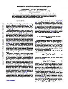
Entanglement is a property that two or more bodies can possess and share. It is a delicate feature created when these bodies interact either directly or via a third party. Their joint correlations are a non-classical attribute, that in no way can be reproduced via local operations and classical communications on either of the bodies. As such, this property is solely of a quantum mechanical origin. When two or more bodies are entangled, they share a fascinating ‘link’, that even when these bodies are space like separated, measurement upon either body determines the outcome of the other. For instance, given two bodies that of which can be in a state of spin-up or down, if one is measured to be in the spin up state, then the other is in the spin-down state (in the case of the conservation of angular momentum). This can be confirmed by observing the latter state which will always have reverted to its classical outcome of spin down. Due to this ‘action at a distance’, the concept of non-locality was introduced, as it is impossible to reproduce these affects by local actions on either system. In fact, Bell’s inequality is a test for non-locality, as entanglement is necessary for nonlocality, with the reverse only being true for two two-level (qubit) systems as proven by Gisin in 1991 [13]. In 2002, Zukowski et al. provided a proof that Gisin’s Thereom could not be generalised to all multipartite (i.e. for more than two) qubit states [14]. A crucial property of entanglement is the ability for a system to be in a superposition of states. That is to say, a combination of two or more classical outcomes at any one time. A conceptual illustration of a superposition can be found in Fig.1.1. Although this is a classical example, the idea of what ‘superposition of states’ actually means may be appreciated. By looking at the initial twelve grid points, some perceive two cubes viewed from a top right elevation, whilst others see two cubes from a lower perspective. In actual fact, both these outcomes can be produced from the initial twelve grid points. Hence, one may rather loosely say that pictorially, the grid points represent both perceptions of two cubes at the same time. Thus, a superposition of both perspectives at once. This is essentially the concept of the superposition of states, only within quantum mechanical terms. For instance, photons can be horizontally ↔ and vertically l polarised. 4

1.2.


¡

¡ ª ¡

@

@ @ R

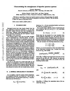
Figure 1.1: A conceptual illustration of what superposition represents. Notice that the grid points can be made into two cubes either viewed from below or from above. Thus, the grid points can be thought to contain both of these perspectives at the same time. By passing an ultraviolet laser beam through a non-linear crystal, such as beta barium borate, both ↔ and l light can be produced. Such a process has been termed type II parametric down-conversion, and is illustrated in Fig.1.2. The cones can be made to overlap, at which point the entangled state of horizontally and vertically polarised photons is produced. This is represented by the overlap of the dashed and solid lines, and the two green cones in Fig.1.2 [15, 16]. The three colours correspond to three different wavelengths implemented in the experiment, of 681nm (blue), 702nm (green) and 725nm (red). The differences between the quantum mechanical and classical possibilities can also be seen by the example of the tossing of a fair coin. Classically the outcome is either heads or tails (assuming it does not land on its rim). In contrast, quantum mechanically the coin is in a superposition of both of these states and so is both heads and tails at the same time, until a measurement is performed at which point the coin will then choose which classical outcome to have. Indeed, there is a probability with which each outcome can occur, but the actual state is not determined until a measurement is performed. Indeed, these examples are reminiscent to a 5

1.2.


Figure 1.2: Entanglement from a non-linear beta barium borate crystal, of type II parametric down conversion [15, 16]. At the point where the two cones of light overlap, entanglement is produced. thought experiment formulated by Schrödinger, known as the Schrödinger cat paradox [1]1 . In this case, a perfectly healthy cat is placed inside a box in which a small quantity of radioactive material is placed and some poison that will be released if the radioactive material decays. Hence, the cat may be dead if the poison were released, or alive if it were not. Nonetheless, without opening the box and making an observation and hence a measurement, one can not say in which state the cat is in, as one does not know if the radioactive decay has occurred. Consequently, the cat is said to be simultaneously dead and alive at the same time. This paradoxical nature of the cat is due to how the microscopic world can effect the macroscopic. Within everyday life, a situation like this is not a sensible one, nonetheless, this is exactly the situation that arises within the quantum mechanical world. The bounds between these two worlds of classical and quantum mechanical rules and possibilities are certainly not clear and well defined [19]. At extremities, which set of rules to use is obvious. However, between these extremes lies a grey area of uncertainty. Nonetheless, the reason why the everyday world is deterministic, as opposed to probabilistic, is due to decoherence. This is the loss of information from a system to the outside world (the environment). The loss of quantum coherence, is the loss of the possibility of superposition for a single body. For two or more bodies, decoherence causes the non-classical entanglement properties to be lost. These states which survive this whole process, are what one perceives in the everyday classical world. 1

A popular account is given within [17] and [18].

6

1.3.

1.3

Why entanglement is studied


With the realisation and acceptance that entanglement does in fact exist, it is now being used as a resource. As bizarre and far from our common perceptions as the results it gives may be, it has given rise to an explosion of research activity. Areas such as quantum communication [20], teleportation [21], quantum cryptography [22], lithography [23] and quantum computation [24, 25] have arisen and expanded. In fact, the future of our technological age relies on entanglement. As mentioned, at the atomic scale, strange effects occur, nothing like there classical counterparts. Instead of a world controlled by facts, it is now probabilistic and undetermined. Inevitably, computers are becoming faster and more sophisticated, but noticeably without increase in size of the machine, or rather machines are getting smaller due to further complexity being placed on the motherboards. This rate of growth of computers was actually predicted by Moore [26, 27] in the form of Moore’s Law which states that the improvement in chip density, and hence in memory size and processor power, will double every eighteen months. As Fig.1.3 shows, this rate has approximately been achieved. The crucial factor, however, is that within the next decade or two, if this drive for faster more powerful computers is to be achieved at the same rate, the circuit boards and chips will then approach the quantum mechanical limit in which one will have to talk about gate operations at the atomic level. The implications are obvious, as classical laws no longer apply. Hence the study of these quantum mechanical effects, such as entanglement and the issue of using it as a resource, giving rise to the quantum computer. Indeed, the incorporation of entanglement has allowed the continued development within lithography where the optical limits due to the frequency of light where being reached [28]. Additionally, with the properties of entanglement, quantum computers have great power due to the mass parallelism achievable due to the possibility of superposition. Nonetheless, the measurement process always results in a single outcome. Consequently, to use properly and effectively the quantum mechanical power that superposition and entanglement gives, requires ingenious experimental setups and measurement processes. With these benefits also comes pitfalls too. The major area of concern is within 7

1.3.


Figure 1.3: Illustration of Moore’s empirical law on the doubling of complexity of the integrated chip every 18 months [26, 27]. cryptography as current security methods for the internet, codes, banking, politics, military etc. are all based on the RSA public key cryptosystem2 3 . Essentially, it is based around the difficulty in factorising a number into its prime factors. For instance, it is a lot easier and quicker to multiple 73 × 41 = 2993 than to find the two prime factors of 27, 561, 1234 . Secure codes use numbers with hundreds of thousands of digits. Even with the fastest computers working in parallel, it would take longer than the age of the universe to factorise them, a long time after anyone is really interested to know what the Prime Minister 2

Named after the co-discovers R. Rivest, A. Shamir and L. Adleman [29, 30]. History has recorded that W. Diffie, M. Hellman and R. Merkle are the inventors of the concept of public-key cryptography, which RSA is based upon. However, due to documents belonging to the British Government now being declassified after 40 years, an alternative history is emerging. Within the Government Communication Headquarters (GCHQ) in the late 1960s, J. Ellis conceived of the idea of sharing information without a secret key. C. Cocks and M. Williamson, also of GCHQ, then found a mathematical way to implement Ellis’ ideas. By 1975, all fundamental aspects of public-key cryptography had been discovered. In the next three years, their discoveries were publicly rediscovered [30]. 4 The answer is 4561 × 6043. 3

8

1.3.


or the President has had for their tea. Classically, the factorisation of a number into its prime constituents is an exponential time dependant problem. Improvement in classical computation has allowed for the complexity of the problem to move along the exponential curve. Thus, although still exponentially dependent on time, the increase in power decreases the time required to factorise a number. Nonetheless, by simply increasing the size of the two prime numbers, the difficulty and time required to factorise the product is again increased, and so security is maintained. With the advent of the quantum computer, an exponential speed up is created in the factorisation and it would then only take a few seconds (given a similar setup to its classical counterpart) to factorise and decode these secure messages, using this method of prime factorisation which the world currently relies on5 . This improvement is due to the classical exponential time dependent problem becoming a polynomially dependent problem. This shift in complexity allows for the exponential speed up and improvement. Hence, all current codes would be broken and information would be freely available to the country with a quantum computer. A frightening situation. The ingenious achievement in both the Shor, the Grover and the Deutsch-Josza algorithms, is the achievement of finding the global property of periodicity, after which the complexity of the problem is greatly reduced. Surprisingly though, the very thing which will bring this security issue into question will also be the cure. Through entanglement, security can not only be restored but improved upon. In no way can a message be penetrated or intercepted without the receiver knowing. In fact, even if the message were intercepted, it would be unintelligible to the third party. Additionally, if the message were then passed on to the original receiver, the intended information could no longer be retrievable, but is forever lost by the involvement of the third party. Due to this delicate nature of entanglement, it is the perfect security for encryption [31]. 5

Taken from an illustration by Peter Knight. Given a 300 digit number to factorise, the best classical algorithm would take 1024 steps and on a classical THz computer, would take 150,000 years. In contrast, Shor’s algorithm takes 1010 steps, but on a quantum THz computer (i.e. same clock speed as classical computer), the factorisation could be completed in less than one second.

9

1.4.

1.4

Types of systems

Types of systems

It is all good and well to talk about entanglement, but it is crucial to understand, manipulate, create and control it, for without these, no real progress can be made. The type and structure of the entanglement also needs to be known. A number of possible candidates for the quantum computer have already been addressed. Di Vincenzo created a check list for which a quantum computer must satisfy [32]. Of all the possible candidates, none satisfy all the requirements or else they are not scalable. Each candidate has advantages, but also disadvantages. The possibilities include nuclear magnetic resonance (NMR), quantum optics, cavity QED, atomic approaches, solid state approaches, ion traps, to name but a few6 . For instance, quantum optics is an established field which can make use of results and experience from many years of research. It is currently implementable within the laboratories, given the present level of technology. However, the scalability of its implementation has been questioned. The various parts required for a quantum computer are available, but as yet the complete sequence has not been created. Looking then at NMR, it has been successful in the actual creation of a quantum computer and has been able to factorise the number fifteen. This may be the smallest product of two prime numbers, but even so, it represents the first major step toward a fully implementable quantum computer. The disadvantage of this method is that it is not scalable to the sizes required for realistic and beneficial calculations to be performed. NMR is essentially limited to approximately 15-20 qubits. Thus, it can only serve as a ‘play thing’, i.e. it is like a hand held calculator in comparison to a computer. The concept and use of quantumness within computation and computers began in the early 1980’s with Deutsch[9] and Feynman[33]. These studies began with the use of qubits (quantum bits) which are in analogue to their classical counterparts of bits, 0’s and 1’s representing off and on respectively. Qubits have the added ability to be superpositions unlike classical bits, i.e. they can be in a classical state of |0i or |1i, or in a superposition such as √12 (|0i + |1i). A pictorial representation of such superpositions is via the Bloch sphere within Fig.1.4. The 6

A road map of the community’s progress can be found at http://qist.lanl.gov .

10

1.4.

Types of systems |0

a|0 + b|1 |1

Figure 1.4: The Bloch Sphere. A representation of all possible superposition a qubit can be in, a |0i+b |1i. The two poles denote the vacuum and excited state, with any other point on the sphere then being a combination of these. two poles represent |1i and |0i, with any other position on the outer sphere then being a superposition a |0i + b |1i, where a and b are defined by the polar angles. Substantial work has been developed in this area, with states having just the two levels of ground and excitation. However, within quantum mechanics, a state can have more than one excitation. Hence, it was not long before d-dimensional systems were investigated. Such systems are termed qudits. This extension from qubits (2) to qutrits (3) and generalisation to qudits was not as straightforward as hoped, with added degrees of complexity arising and key theorems not being generalisable to d dimensions. These included the representation of the Bloch sphere and Gram-Schmidt method. Quantum optics is a more developed field of research, as well as being substantially more experimentally viable. However, light has an infinite dimensional Hilbert space. With the difficulties surrounding the extension of ideas and formulae from 2 to d dimensions, the understanding of infinite dimensional systems within entanglement seemed a long way off. Nonetheless, it turned out that coherent states of infinite dimensional systems are indeed comprehendible due to their Gaussian statistics. For Gaussian systems, (i.e. states which remain Gaussian even after being operated on), a separate area of research has emerged, of different notation and thought to finite dimensional systems. It is within this area that the work presented here is involved in. 11

1.5.

1.5

Motivation and Outline


Within this thesis, the work presented will mainly deal within the quantum optics regime. That is, we deal with an ideal gas of bosons for which each state is termed a mode or coherent state and due to the infinite degrees of freedom that each of these modes can have, (from their infinite dimensional Hilbert space), they correspond to continuous variable (CV) systems. Linear and non-linear interactions can be performed on these modes. For instance, a half silvered mirror (beam-splitter) is a linear device whilst a nondegenerate parametric amplifier is a non-linear device. A beam-splitter both transmits and reflects light, like a window does with approximately 4% of light being reflected and 96% being transmitted. Linear and non-linear devices are differentiated by whether or not they are linear in their annihilation and creation operators, a ˆ and a ˆ† respectively, i.e. a â ˆ† is still linear but a ˆ2 is non-linear. Experimentally, many states such as squeezed, number, thermal, and coherent states can be created given present technology. Of interest here will be the squeezed state, as they are created by non-linear optical processes including optical parametric oscillation and four-wave mixing, and so therefore contain entanglement. It will be from both the single-mode and two-mode squeezed states that many of the scenarios will be developed from. Within the last few years analytic criteria for Gaussian CV systems have emerged (see Chapter 2 for an explanation of this background theory). It mainly deals with simple two body (or mode) interactions and how to characterise the entanglement structure of the overall system. Additional, measures for the amount of entanglement shared between any two modes has been formulated. Nonetheless, beyond the direct interaction of two modes, less is known, both in regard to the entanglement structure of the overall system and the amount of entanglement shared between different combinations of groups (with a limit of two groups). To better understand this gap in knowledge, my research has been within multipartite (or many-mode) CV systems. I have studied Gaussian systems through their entanglement structure, that is, by looking at the pairwise entanglement, 12

1.5.


the entanglement between one and many modes, and between two groups of M and N modes. Through this process, a fuller comprehension of a systems details can be pieced together. Additionally, the purity of the system and the amount of entanglement in the system has been investigated, under certain configurations given certain measures. Furthermore, within CV systems, due to the infinite degrees of freedom that they possess, they are more susceptible to the noise of the environment which surrounds it. Consequently, the mechanism of decoherence and how it alters and eventually degrades the entanglement of a system has also been investigated, both within the Markovian approximation and beyond. The issue of quantum computation requires the need for distribution of entanglement as well as storage and manipulation. Through the study of decoherence, with a better understanding of this complex process, measures to overcome or minimize its effects can be developed. The ability to distribute entanglement in an effective, hassle-free manner would be advantageous to many. Just such a configuration will be outlined in Chapter 5 in which only a good initial setup of the entangled state and the time of the global evolution of the total system are required. The outline of my thesis is as follows. Chapter 2 will detail theory, previously developed by others and which will be used within calculations and explanations of results. As such, it covers all background theory required to understand and comprehend the investigations presented here. Chapters 3-5 incorporate the main results of this thesis. Chapter 3 will begin with a description of the decoherence process, in which the environment acts upon a system. The derivation of the master equation will be outline in the case of the Born-Markov approximation, and how this can in turn be incorporated into the development of the master equation beyond such an approximation. This therefore allows the evolution of the system to include memory effects of previous interactions. Within the Born-Markov approximation, the environment would always relax back to its original state, and so each interaction of a system with its surrounding environment is independent of the next. It will be shown how, 13

1.5.


with the collective approach, the complete positivity of the reduced dynamics can be guaranteed. Sections of this have been accepted for publication in J. Mod. Opt. (2005), as well as being published in Phys. Rev. A 70, 024301 (2004). Chapter 4 details how the Markovian approximation can be incorporated and modelled. The idea of the collective mode will also be presented in a more detailed form, as well as being utilized. The main result of this chapter centres around how many body entanglement is created upon an environment interacting with one mode of a two-mode non-classical state, firstly by considering a twomode squeezed state and then including the possibility of local squeezing. This work has also been published in Phys. Rev. A 68, 063814 (2003) and J. Korean Phys. Soc. 44, 691, Part2 (Mar 2004). Chapter 5 consequently deals with going beyond the Markovian approximation to the non-Markovian regime through an investigation of a general interaction Hamiltonian, which governs the evolution of the system, is decomposed into simple linear interactions in the case of resonant interactions. Such an interaction Hamiltonian can be a representation of non-Markovian decoherence, as the order of interaction is never specified. Additionally, the result is explained in the context of quantum distribution and shown to be efficient in the distribution from one state to many. The work of Chapter 5 has been published in Phys. Rev. Lett. 94, 070501 (2005), as well as some sections having been accepted for publication in J. Mod. Opt. (2005). Lastly, a summary of the results and conclusions drawn will be presented in Chapter 6. In addition, possible future extensions and directions of study will be commented on.

14

Chapter 2

Background Theory

15

2.1.

Basic Concepts: Separable or Entangled? “For the things of this world cannot be made known without a knowledge of mathematics.” - Roger Bacon, Opus Majus (pt. 4)

2.1

Basic Concepts: Separable or Entangled?

A composite quantum system is one which consists of a number of quantum subsystems. If and when these subsystems are entangled, it is not possible to assign to each individual subsystem a definite state vector. Thus, entanglement is a property that two or more bodies can possess, such that, even though they are space like separated, they share joint information/correlations that can not be fully obtained by local observations of either body. Additionally, local operations and classical communication (LOCC) on either subsystem can never produce entanglement nor increase it (if entanglement is already present). Therefore, any quantum state must either be entangled or separable, no other possibilities exist. Consequently, a bi-separable state is defined as a state that can be written as a convex combination of product states. That is, it is created by two completely separate, independent systems. Hence a measurement on A does not affect B or vice versa. If the state cannot be written in this manner, it is said to be entangled. A bi-separable state can therefore be written as %ÂB =

X

pi %Âi ⊗ %ˆBi ,

(2.1)

i

where %ÂB , %îA and %îB are respectively the density matrices for the composite system AB and the two independent systems of A and B which occur with P probability pi , where 0 6 pi 6 1 and i pi = 1 [34]. A density matrix (or operator) %ˆ simply serves as a different notation for a state vector |Ψi within quantum mechanics. For a pure state |Ψi, its density density operator is defined as %ˆ = |Ψi hΨ|. Otherwise, the state is termed mixed, as incomplete knowledge of |Ψi exists and %ˆ can only be represented as an ensemble of pure states, each

16

2.1.

Basic Concepts: Separable or Entangled?

occurring with probability pi such that, %ˆ =

X

pj %ˆj = p1 |Ψ1 i hΨ1 | + p2 |Ψ2 i hΨ2 |

(2.2)

j

P with 0 6 pj 6 1 and j pj = 1. Consequently, in Eqn.(2.1) if pi = 1, the state would be pure and separable whilst for pi < 1, the state would be mixed and separable. Pictorially or conceptually, pure and mixed states can be described in the following manner. Assume that a state may be represented by white and blue spheres in a box as illustrated in Fig.2.1, where white and blue represents the two possible outcomes that a state may have, in analogue to 0 and 1 for a qubit. As depicted in Fig.2.1(a), a state which is pure will, before measurement, all be in the same state and hence all are coloured both white and blue. If the state of each ball where |Ψi = √12 (|bi + |wi), where |bi denotes a blue coloured ball and similarly |wi is white, then there is equal probability that all balls will be coloured white as blue. However, until a measurement is performed, the colour that they possess is unknown. Nonetheless, by measurement upon just one of the balls, the colour of all of them is identified. This is similar to the fact that all knowledge of |Ψi is known for a pure state, that is, the colour of all the spheres is known. It must be noted that by measurement upon a single ball, its state will have changed. In contrast, Fig.2.1(b) demonstrates pictorially a mixed state. In this instance, the state is formed from a mixture of colours, half white and half blue in this example. This is the greatest mixture of two colours that there can be and so entropy is at its greatest (a pure state has zero entropy). In this case %ˆ = 12 (ˆ %b + %ˆw ). Notice how the state can only be described using an ensemble of pure states, due to the two different wave functions that the state may have from the two possible colours. Given such a straightforward definition as Eqn.(2.1) for a system to be separable into two parts, the difficulty arises in proving whether such a representation is indeed possible or not. This is a non trivial matter and hence other means to discern separability of a system are required. From this a number of issues arise. Firstly, the dimension of the system in question will alter the criterion used, be it for 2 level qubit states, d dimensional qudit systems or infinite dimensional 17

2.1.

Basic Concepts: Separable or Entangled? (a)

(b)

Figure 2.1: Conceptual illustration of a pure or mixed state. (a) depicts a pure state as all spheres are the same colour, a combination of blue and white, which upon measurement will take a specific colour. (b) is a mixed state in which here half the spheres are in one colour (white) and half the other (blue), and so has been formed from a mixture of two pure states. Hilbert spaces in which continuous variable (CV) systems exist. Secondly, depending on whether the complete system is pure or mixed, this has a large impact on how the entanglement is detected. Lastly, the number of parties to be considered and how these are divided into groups again has an affect. For instance, Eqn.(2.1) dealt with bi-separability of a composite system. However, given three bodies A, B and C, there are a number of possible divisions: A − BC, B − CA, C − BA, A − B, A − C, B − C and A − B − C where − denotes a division. Indeed, there can be entanglement between AB, AC, BC and/or ABC or various combinations of these. For N subsystems there are a total of 2N −N −1 different possible ways that the system can be entangled. Thus, the task of observing, classifying and understanding entanglement is not a straightforward one. Before this is discussed further, the notation that will be used throughout this thesis will be detailed.

18

2.2.

CV Notation and Terminology

2.2

Notation and Terminology for CV Systems “Philosophy is written in this grand book – I mean the universe – which stands continually open to our gaze, but it cannot be understood unless one first learns to comprehend the language in which it is written. It is written in the language of mathematics, and its characters are triangles, circles, and other geometric figures, without which it is humanly impossible to understand a single word of it; without these, one is wandering about in a dark labyrinth.” Galileo Galilei (1564-1642)

The following Section consists of the notation and basic results and relationships that will be used throughout the remainder of these Chapters.

2.2.1

Operators and States

As mentioned, a composite quantum system contains a number of quantum subsystems. These subsystems are often referred to as modes within CV systems, as each individual subsystem of one body is a mode of light. For a mode denoted by a, it will have creation and annihilation operators a ˆ† and a ˆ respectively which † † † have the Bose commutation relation [â, a ˆ ] := a â ˆ −ˆ aa ˆ = 1. These in turn can be qˆ + iˆ p qˆ − iˆ p † defined within phase space as a ˆ= √ and a ˆ = √ with the commutator 2 2 relationship [ˆ q , pˆ] = i, where (q, p) is position and momentum. This definition for the operators was introduced as far back as 1928 by Fock [35], together with the number operator n ˆ =a ˆ† a ˆ, where |ni are known as the ‘Fock states’. These operators are such that when acting upon the Fock number states |ni, a ˆ† |ni = (n + 1)1/2 |n + 1i and a ˆ |ni = n1/2 |n − 1i where a ˆ reduces the number of † quanta by one whilst a ˆ increases it by one, as suggested by their names. Note a ˆ acting on the vacuum state has the result, a ˆ |0i = 0. A few basic forms of states are listed below:

19

2.2.


Vacuum state |0i: This is the state of nothing. There is no added noise or heat as it represents the ground state, n = 0. Classically this would be a point at the origin, but within phase space it is depicted as in Fig.2.2, where the area represents the uncertainty of the state’s phase and amplitude. Fig.2.3 again illustrates the vacuum state but from a different perspective. Thermal field ρˆn¯ : n ¯ is the average number of photons at temperature T such that · µ ¶ ¸−1 ~ω n ¯ = exp −1 , (2.3) kB T where kB is the Boltzmann constant and ω is the frequency. The density matrix for a thermal field will be denoted by %ˆn¯ and for brevity n ˜ = 2¯ n+1 will be used. A thermal state density operator can therefore be written as, %ˆn¯ =

exp (−H/kT ) , Tr [exp (−H/kT )]

(2.4)

given a Hamiltonian H.This is the state of least knowledge and so the most noise of the two quadratures. Consequently this state has the largest area in phase space and only the mean value of energy is known. Such a state is frequently used as a model for an environment in equilibrium at temperature T . This will be the case in Chapters 3 and 4. Coherent states |αi: This is produced by the action of the Glauber displacement operator upon a vacuum state, ˆ |αi = D(α) |0i , ˆ D(α) := exp(αˆ a† − α∗ a ˆ),

(2.5a) (2.5b)

ˆ † (α) = D(−α) ˆ ˆ −1 (α). A where α = |α| exp(iϑ) = αr + iαi and D = D coherent state contains the least uncertainty over the two quadratures, as illustrated in Figs.2.2 and 2.3, with non-zero amplitude |α| and phase ϑ. Classically, this would be a point, quantum mechanically it is depicted by a circle as the uncertainty in both quadratures is the same. The name ‘coherent state’ was presented in literature for the first time in 1963 by Glauber [37] where he showed that a ˆ |0i = α |αi and in a title in Ref.[38], although many other authors had previously considered similar work [35]. 20

2.2.


Figure 2.2: An illustrative gallery of quantum states within phase space reprodced from Ref.[36]. The two axes represent the two quadratures (q, p) where the area represents uncertainty, here the minimum uncertainty. Shown are a vacuum state, a coherent state, a squeezed vacuum state and three bright squeezed states with different phase angles. In fact, the definition of Eqn.(2.5) was used by Feynman and Glauber as far back as 1951 [35, 39]. Coherent states are considered the most ‘classical’ of pure quantum states [40] and serve as a good starting point in the creation of ‘non-classical states’ [37, 38]. Squeezed States: These are non-classical states created from the single-mode squeezing operator Sâ or the two-mode squeezing operator Sâb . The singlemode squeezing operator is defined as µ

¶ ∗ ξ ξ †2 2 Sâ (ξ) := exp − a ˆ + a ˆ , 2 2

(2.6)

where ξ = s exp(iϕ) and is normally referred to as the squeezing parameter. This is similar to the displacement operator, although it is now non-linear ˆ ˆ in the bosonic operators. Again S(ξ) is unitary as Sˆ† (ξ) = S(−ξ) = Sˆ−1 (ξ). When acting on the vacuum state, the single mode squeezed state is produced ˆ |0i := |ξi . S(ξ) (2.7) Fig.2.2 illustrates such a state where the knowledge of one quadrature has been increased and so the other is correspondingly decreased, so that the area of uncertainty before and after squeezing is maintained. Within 21

2.2.


Figure 2.3: This is an alternative perspective showing amplitude and phase obtained from Ref.[36]. Comparisons to Fig.2.2 again shows how the squeezing of a quadrature can decrease the uncertainty in one quadrature, but the other is then less well defined, and so maintaining the overall limit of knowledge.

22

2.2.

CV Notation and Terminology Figs.2.2 and 2.3 a squeezed vacuum is illustrated. The two-mode squeezed state (TMSS) of modes a and b with annihilation operators a ˆ and ˆb respectively, is generated by the action of the two-mode squeezing operator on a two-mode vacuum state |ξiab := Sâb |00i , ³ ´ Sâb := exp −ξˆ a†ˆb† + ξ ∗ a ˆˆb ,

(2.8a) (2.8b)

with once again ξ = s exp(iϕ). Note however that this is not simply a product of two single mode squeezing operators. Both Sâ and Sâb are nonlinear in nature, however Sâ is associated with degenerate process whilst Sâb is formed within non-degenerate (energy conserving) processes. Each of these states can be used and manipulated in various ways. To introduce ˆ a (ϑ) a phase ϑ into a system, for example to a mode a, the rotation operator R is applied where ˆ a (ϑ) := exp(iϑˆ R a† a ˆ). (2.9) This is a local operation and so when applied to a state, will not contribute to the amount of entanglement within a system. However, it may be used to manipulate it, after entanglement is created by other means. Additionally, mirrors may be used to redirect the light source through the appropriate apertures. The phase of a field will be shifted by π.

23

2.2.

CV Notation and Terminology c

b

d

a

Figure 2.4: A diagram of a beam-splitter showing how the two output fields are a result of both the reflected and transmitted input fields. Beam-Splitters If however, the mirror is not 100% reflective, it is referred to as a beam-splitter. Fig.2.4 diagrammatically shows how it can superimpose the two input modes into the output modes by cˆ = tˆ a + rˆb, (2.10a) dˆ = rˆ a + tˆb,

(2.10b)

in which |r|2 and |t|2 are the complex reflectivity and transmittivity respectively, and which must satisfy |t|2 + |r|2 = 1 and rt∗ + r∗ t = 0 so that the commutation ˆ dˆ† ] and [ˆ ˆ cˆ† ] are maintained. relations [ˆ c, cˆ† ] = 1 = [d, c, dˆ† ] = 0 = [d, The superposition of modes a ˆ and ˆb is linear, however beam-splitters can again manipulate entanglement. The beam-splitter operator in its most general form is given by [41] h ³ í iϕ †ˆ −iϕ ˆ† ˆ Bab (φ, ϕ) := exp φ e a ˆ b−e a ˆb ,

(2.11)

where ϕ is the phase shift between reflected and transmitted fields and φ controls † the values for reflectivity and transmittivity, and is such that cˆ = Bâb a ˆBâb = † ê−iϕ sin φ, where r = eiϕ sin φ, a ˆ cos φ + ˆbeiϕ sin φ and dˆ = BâbˆbBâb = ˆb cos φ + a r∗ = e−iϕ sin φ and t = t∗ = cos φ which is taken real without loss of generality1 . 1

In the case of real values for reflectivity and transmittivity, (i.e. ϕ = 0) Eqn.(2.10b) must become dˆ = −rˆ a + tˆb, whilst Eqn.(2.10a) remains the same. This requirement comes from the † fact that the operators must be unitary, and so Bâb Bâb = 11. Whether a complex or real beam-

24

2.2.

2.2.2


The Characteristic Function

Within CV systems, significant headway has been achieved for Gaussian states, as it is these types of states that are (relatively easily) produced by linear opˆ ˆ ˆ ϕ) tics, squeezing and homodyne detection. The operators D(α), R(ϑ) and B(φ, are contained within linear optics whilst Sâ and Sâb are squeezing operators. Homodyne detection is simply a tool for measuring a quadrature to near unit efficiency [42]. These Gaussian states possess a Wigner function W [43, 44, 45], which is everywhere positive and can be calculated from the Weyl characteristic function χ(η, ζ) via the Fourier Transformation 1 W (α, β) = 2 π

Z χ (η, ζ) exp (η ∗ α − ηα∗ ) exp (ζ ∗ β − ζβ ∗ ) d2 η d2 ζ,

(2.12)

where α = αr +iαi , β = βr +iβi , η = ηr +iηi and ζ = ζr +iζi , with the subscripts r and i denoting real and imaginary parts respectively. This was the first quasiprobability distribution introduced into quantum mechanics by Wigner [43]. The characteristic function in the case of a two-mode system is itself defined as h i ˆ a (η)D ˆ b (ζ) %ˆ , χ(η, ζ) = Tr D

(2.13)

ˆ is the displacement where x = (η, ζ) are the coordinates for two modes and D operation. If χ(η, ζ) is known, %ˆ may be determined and vice versa. For Gaussian states, χ(η, ζ) = χ(x) can take an alternative, equivalent form of ·

¸ ¢ 1¡ T T χ(x) = exp − xVx − id x , 2

(2.14)

which depends solely on the first and second moments of the quadratures. Here d is the linear displacement, V the variance (or correlation or covariance) matrix and x is the coordinate vector of the quadratures. The elements are determined by the mean quadrature values of the field, Vij = h(ˆ xi xˆj + xˆj xî )i which uniquely represent the entanglement nature of a Gaussian field as displacement terms can splitter is being considered will always be clear from the context. Indeed, the beam-splitter will be taken as real, with the exception within Chapter 5 when both forms are required.

25

2.2.


be removed by local actions and so do not play a crucial role. The variance matrix for the various states previously outlined will now be given. A single mode state will be represented by a 2 × 2 matrix whilst an n mode state will have a 2n × 2n correlation matrix. The TMSS will be explicitly calculated below for illustration, whereas the others will simply be given in Table 2.1. Derivation of the variance matrix for a TMSS. The TMSS is created by Eqn.(2.8) † %âb = Sâb |00i h00| Sâb ,

(2.15)

´ ³ ˆ a (α)D ˆ b (β) Sâb |00i h00| Sˆ† χab (x) = Tr D ab

(2.16)

† ˆ † ˆ Db (β)Sâb |00i , Da (α)Sâb Sâb = h00| Sâb

(2.17)

and so by Eqn.(2.13)

† by the use of Sâb Sâb = 11 and the cyclic properties of the trace, with x = (α, β) = (αr , αi , βr , βi ). By use of the relationships

£ ¤ ˆ ˆ −A ˆ ˆ + [A, ˆ B] ˆ + 1 A, ˆ [A, ˆ B] ˆ eA Be = B 2! 1 h ˆ £ ˆ ˆ ˆ ¤i + A, A, [A, B] + . . . 3! µ ¶ θ2 ˆ ˆ ˆ ˆ ˆ ˆ exp[θ(A + B)] = exp(θA) exp(θB) exp − [A, B] 2

(2.18) (2.19)

then † Sâb a ˆSâb = a ˆ cosh s − ˆb† eiϕ sinh s, † ˆˆ Sâb bSab = ˆb cosh s − a ˆ† eiϕ sinh s.

(2.20) (2.21)

The relationships of Eqns.(2.18) and (2.19) are frequently applied in calculations and a proof of their validity is provided in Appendix A. By the above and along with the definition in Eqn.(2.8b), one can calculate ˆ a (α)Sâb and Sˆ† D ˆ b (β)Sâb . Through the use of the exponential nature of the Sˆ† D ab

ab

26

2.2.


† displacement operator (2.5b), the Taylor expansion and the use of Sâb Sâb = 11, † ˆ ˆ a (α cosh s)D ˆ b (α∗ eiϕ sinh s), Sâb Da (α)Sâb = D † ˆ ˆ b (β cosh s)D ˆ a (β ∗ eiϕ sinh s). Sâb Db (β)Sâb = D

(2.22) (2.23)

Hence, substituting Eqns.(2.22) and (2.23) into Eqn.(2.17) results in ˆ a (α cosh s + β ∗ eiϕ sinh s)D ˆ b (α∗ eiϕ sinh s + β cosh s) |00i χab (x) = h00| D = h00| α cosh s + β ∗ eiϕ sinh s, α∗ eiϕ sinh s + β cosh si µ ¶ 1 ∗ iϕ 2 = exp − |α cosh s + β e sinh s| 2 ¶ µ 1 ∗ iϕ 2 × exp − |α e sinh s + β cosh s| 2 · h i¸ 1 2 2 −iϕ ∗ ∗ iϕ = exp − cosh 2s(|α| + |β| ) + sinh 2s(αβe −α β e ) 2 · 1 = exp − cosh 2s(αr2 + αi2 + βr2 + βi2 ) 2 ¸ − sinh 2s(αr βr − αi βi ) , (2.24) where the last equality has been obtained by taking real values for the squeezing parameter, i.e. ϕ = 0. Recalling the equivalent form for the characteristic function given by Eqn.(2.14), where now displacement terms are neglected, ·

¸ 1 T χab (α, β) = exp − (αr , αi , βr , βi ) V (αr , αi , βr , βi ) , 2

(2.25)

then by comparison of Eqns.(2.24) and (2.25), the various elements of V can be determined. For instance, the coefficient of αr2 will give its value to the element V11 and as αr αi = αi αr ⇒ V12 = V21 , we obtain  VT M SS

  =  

cosh 2s 0 sinh 2s 0 0 cosh 2s 0 − sinh 2s sinh 2s 0 cosh 2s 0 0 − sinh 2s 0 cosh 2s

   .  

(2.26)

In a similar manner, the variance matrices for the other states can be determined 27

2.2.

CV Notation and Terminology State or operator Two-mode vacuum state Two-mode thermal state Single-mode squeezed state Two-mode squeezed state Beam-splitter

Variance Matrix µ ¶ 11 0 µ 0 11 ¶ n ˜ 11 0 ˜ 11 µ 0 n ¶ cosh s sinh s µ − sinh s cosh s ¶ cosh 2s11 sinh 2sσz µ sinh 2sσz ¶cosh 2s11 t11 −r11 r11 t11

Table 2.1: Variance matrices for the two-mode vacuum, two-mode thermal, single-mode squeezed and the two-mode squeezed states as well as the beamsplitter operator in the case of real transmittivity and reflectivity. 11, 0, and σz are the 2 × 2 identity, zero and z-Pauli matrices respectively. to give the results presented in Table 2.1.

2.2.3

Different Types of Entanglement

Certain types of entanglement have been assigned various names after the codiscoverers, for instance the GHZ state is named after Greenberger, Horne and Zeilinger [46], or the W-state after Wootters [47]. Both describe tripartite (three body) entanglement, but nonetheless there are subtle differences. A GHZ state is such that subsystems A, B and C are fully entangled yet upon measurement of any one of these, the remaining two subsystems will no longer be entangled, i.e. there is no pairwise entanglement. A good way to visualize such a state is with the Borromean Rings [48] as illustrated in Fig.2.5. These rings are such that whilst all three are connected, the removal of one leaves the remaining two no longer connected, regardless of labelling. In contrast a W-state retains the joint correlations of the pairwise entanglement of the two remaining subsystems after measurement upon the third, as well as being initially fully entangled. For qubit systems, these are denoted respectively by |ψiGHZ = √12 (|000i + |111i) and |ψiW = √13 (|100i + |010i + |001i). Indeed, the entanglement of a composite system of N bodies is highly complex, with many different configurations possible. Consequently, there exists criteria which can only infer if the composite

28

2.2.


Figure 2.5: The Borromean Rings [48]. Removal of just one ring leaves the remaining two no longer connected. This is in analogue to the GHZ states, where measurement upon any one subsystem leaves the remaining two no longer entangled, even though all three where initially entangled. system contains entanglement or not, without knowledge of the distinct form the entanglement of the system has nor the amount present. The next two Sections detail entanglement criteria for the finite dimensional system and the CV systems respectively. This is then followed by a Section on the problems of classification and measurement of the amount of entanglement within a composite system, and under certain situations what is achievable.

29

2.3.

2.3

Entanglement Criteria I

Entanglement Criteria: Finite Dimensional Systems

The following contains a brief outline of the separability criteria used for finite dimensional systems. Firstly, bi-separability of pure states will be considered, both for two-dimensional systems via the reduced density matrix and for systems of dimension N and M where the Schmidt decomposition is used. This will be followed by details of bi-separability of mixed states which will be explained briefly both in the case of two subsystems and beyond.

2.3.1

The Reduced Density Matrix

If the system is initially in a pure state, separability conditions are not too difficult to handle. For instance, given a two body state |Ψiab = |↑ia |↑ib , is this state entangled? In this illustration, ↑ represents spin up whilst ↓ is spin down, as would be the case for magnetic spin of an atom. To answer this question, one can look at the reduced density matrix which is when part of a system has been traced over. For example, %â = Trb %âb and %ˆb = Tra %âb where Tra denotes the partial trace over subsystem a. Essentially, the reduced density matrix %â is a description for the state of system a. Given the above state %âb = |Ψiab hΨ| = |↑ia h↑| ⊗ |↑ib h↑|

(2.27)

by commutation relationships. Thus, upon removal of subsystem b, the reduced density matrix of the remaining system a is %â = Trb %âb = |↑ia h↑| .

(2.28)

In this instance %â is in a pure state as only a single wave function is required to describe the subsystem a. This indicates that the initial system was separable as the measurement upon one subsystem has had no effect on the other. Therefore 30

2.3.


the initial system could have been written as a product state of two independent subsystems, as is evident from Eqn.(2.27), i.e. %âb = %â ⊗ %ˆb . If instead, one where to consider the pure state case %âb =

√1 (|↑i a 2

|↑ib + |↓ia |↓ib ) in which

1 (|↑ia h↑| ⊗ |↑ib h↑| + |↑ia h↓| ⊗ |↑ib h↓| 2 + |↓ia h↑| ⊗ |↓ib h↑| + |↓ia h↓| ⊗ |↓ib h↓|)

(2.29)

By tracing over subsystem b, the reduced density matrix for subsystem a will be %â = Trb %âb 1 = (|↑ia h↑| + |↓ia h↓|) 2

(2.30)

as Trb |↑ib h↓| = b h↓| ↑ib = 0 by orthogonality. In this instance %â is a mixed state as it must be written as an ensemble of wave functions. Consequently, the initial state of %âb must have been entangled, as the tracing over of one subsystem has affected the other indicating that they were not originally independent of each other. The state of the joint system was initially a pure state and so known exactly, however by considering only subsystem a (or b), as it has become a mixed state, one no longer has maximal knowledge of the individual parts of the system. Hence, some joint correlation between subsystems must have been present. In summary, given an initial pure system of two parties (or groups), the tracing over of one party can reveal if the initial system was entangled. If the remaining system is in a pure state, this indicates that the initial system contained two independent subsystems and so were separable, whilst in the case of a mixed state this indicates that the two subsystems were not independent and hence entangled.

31

2.3.

2.3.2


The Schmidt Decomposition

The previous Section dealt with a composite system containing two subsystems, each with two possible outcomes (spin up and spin down) so that it had dimension two. However, the Schmidt decomposition provides necessary and sufficient conditions for the separability of a pure composite state %ÂB ∈ HA ⊗ HB , where A and B are two subsystems [49]. Given that dim HA = M and dim HB = N with M 6 N , then the Schmidt decomposition shows that any state can be written as |ΨiAB =

r X

ci |ui i |vi i ,

(2.31)

i=1

where {|ui i} and {|vi i} form orthonormal basis for subsystems A and B and P ci are the Schmidt coefficients with ci > 0 and i c2i = 1. Accordingly, upon tracing over either subsystem, the reduced density matrix (in the Schmidt basis) is diagonal and both %Â and %ˆB have positive identical eigenvalues c2p as %Â = TrB %ÂB X = ci cj |ui i huj | ⊗ hvi |vj i i,j

=

X

c2p |up i hup |

(2.32)

p

P and similarly %ˆB = p c2p |vp i hvp |. Additionally, when a subsystem is of dimension M , it can only be entangled with at most M orthogonal states of the other subsystem. Within Eqn.(2.31), r is the Schmidt rank where r 6 M . It is from this number that the bi-separability of the system is determined as the two subsystems are bi-separable ⇔ r = 1, otherwise they are entangled. Note that if r = 1 then |ΨiAB = |ϕiA |φiB , as was required in Eqn.(2.1) for a pure state given that pi = 1 . For more than two subsystems the Schmidt decomposition is in general impossible as shown in [50]. Additionally, for mixed states the Schmidt decomposition no longer exists. Instead alternative methods are required, as will be discussed next.

32

2.3.

2.3.3


Separability Criteria for Mixed States

As a mixed state signifies incomplete knowledge of the state, the purity/mixedness of the state can no longer be used to observe the presence of joint correlations between subsystems. Instead the following, in decreasing order of strength provide entanglement criteria: • Peres-Horodecki Criterion: Positive Partial Transpose (PPT) [51, 52, 53] • Reduction Criterion [54, 55] • Majorisation Criterion [56] A comparison of the latter two can be found in Ref.[57].

Positive Partial Transpose This criterion was proposed by Peres [51] and later proven to be both necessary and sufficient by the Horodecki’s [52, 53] for the bipartite separability of qubitqubit (2 × 2) and qubit-qutrit (2 × 3) systems. For higher dimensional systems the necessary condition is no longer a sufficient one. It is based upon the fact that partial transposition (PT) takes separable density operators necessarily into a non-negative density operator. That is, PT is a positive mapping, but not completely positive [109]. Therefore, if one assumes that the initial state is separable, and after PT the state is no longer positive, the original assumption of separability was incorrect. Hence positive partial transposition (PPT) indicates separability and negative partial transposition (NPT) indicates entanglement of the bipartite system. Partial transposition is where only a section of the system is transposed, for example, %ˆT2 is the PT of the subsystem labelled 2. Thus for P P %ˆ12 = i %î1 ⊗ %î2 , then PT of system one is %ˆT121 = i (ˆ %i1 )T ⊗ %î2 . To be a valid density operator, %ˆ must be non-negative and have unit trace. Consequently, if after PT this is not the case, it signifies that the initial system was non-classical and could not be written in product form. The eigenvalues of %ˆT2 identify this positivity, as if one or more eigenvalues are negative, this implies the state is not completely positive and so must be entangled. 33

2.4.

Entanglement Criteria II

2.4

Entanglement Criteria: Infinite Dimensional Systems

CV systems are now considered, with the criterion presented below only being valid for Gaussian systems unless otherwise indicated. For the separability of bipartite systems, two independent methods appeared in the same journal (Physical Review Letters) at the same time (2000), one was by Simon [58], the other by Duan et al. [59]. Both methods can be employed, but it will be Simon’s criterion that will be presented below and used throughout.

2.4.1

Simon’s Criterion

Extending the Peres-Horodecki necessary and sufficient criterion beyond 2 × 2 and 2 × 3 dimensional bipartite systems, there exists bound entangled states, that is bipartite entangled states which have PPT. (A detailed explanation of these will follow in the next Section). Nonetheless, Simon was able to show that the Peres-Horodecki criterion was indeed a necessary and sufficient condition for bipartite CV Gaussian systems by the following logic.

• Firstly, note that by taking the partial transpose of a state, this is equivalent to a mirror reflection in phase space upon the section the PT is carried out on. That is, the phase space coordinates (q, p) → (q, −p) ⇔ %ˆ → %ˆT . • Secondly, for a bipartite system of two modes a1 and a2 with annihilation operators a ˆ1 = as

qˆ1√ +iˆ p1 2

and a ˆ2 =

qˆ2√ +iˆ p2 , 2

these can be written more compactly

ζ = (q1 , p1 , q2 , p2 ) and ζˆ = (ˆ q1 , pˆ1 , qˆ2 , pˆ2 )

(2.33)

(with obvious extension for N modes). The commutation relation [ˆ qi , pˆj ] = iδij can also be written in compact form via the 4 × 4 matrix Ã [ζˆα , ζˆβ ] = iJαβ , J2 = J ⊕ J, J =

0 1 −1 0

! .

(2.34) 34

2.4.

Entanglement Criteria II The subscript 2 on J here indicates the two modes of the system. When and where the number of modes of the system is obvious, this subscript will be dropped. Partial transposition of the second mode will then have the effect that ζ → Λζ = (q1 , p1 , q2 , −p2 ) (2.35) with Λ = diag(1, 1, 1, −1), whereas PT over the first mode would have resulted in Λ = diag(1, −1, 1, 1). That is, the pi quadrature of the appropriate mode goes to −pi .

• Thirdly, for a state to be physically possible, it must always satisfy the uncertainty principle [60]. This in turn can be expressed through the variance matrix whose elements are the second moments or uncertainties of the state where, as noted earlier, Vαβ = h{∆ζˆα , ∆ζˆβ }i, ∆ζˆα = ζˆα − hζˆα i and {x, y} := xy + yx is the anti-commutator (or in case of classical variables the Poisson bracket). Thus, the uncertainty principle can be written as V + iJ2 > 0

(2.36)

where V and J2 are both 4 × 4 matrices. • Fourthly, upon PT of a mode, if the state was indeed separable, it must still satisfy the uncertainty principle, both before and after PT. However, if the state was entangled, then the uncertainty principle no longer holds after PT. Due to the PT being a mirror reflection in phase space, it has ˜ = ΛVΛ. Hence if after PT the effect to transform V into V ˜ + iJ > 0 V

(2.37a)

then the system is separable, whereas if ˜ + iJ < 0 V

(2.37b)

it is entangled. Alternatively, one may write this condition in the equivalent form of ˜ > 0 where J ˜ = ΛJ2 Λ = J ⊕ (−J) V + iJ (2.37c) if the system has two modes, where here the latter mode was partial trans35

2.4.

Entanglement Criteria II posed. This is often a more convenient form than Eqn.(2.37a), as the ˜ is easily obtainable for whatever variance matrix is unchanged whilst J mode the partial transposition is over.

• The variance matrix can be written in a 2 × 2 block matrix form Ã ! A C V= , CT B

(2.38)

where each block can be transformed into a standard form such that A, B and C are diagonal. (See Duan for more details [59]). • By Symplectic properties of Sp(4, R ), the Peres-Horodecki condition may be again re-written in an Sp(2, R ) ⊗ Sp(2, R ) invariant form, where det A, det B, det C and Tr(AJCJBJCT J) are all invariant. For an overview of the properties that symplectic groups have, see Appendix B. Therefore an equivalent form of the uncertainty principle of Eqn.(2.36) is det A det B + (1 − det C)2 − Tr(AJCJBJCT J) > det A + det B. (2.39) ˜ = ΛVΛ. In other words On taking the PT of the second mode,V → V C → Cσ3 , B → σ3 Bσ3 and A remains unchanged, where σ3 = diag(1, −1) is the z-Pauli matrix. All invariants remain unchanged except det C which is now det(Cσ3 ) = − det C. Consequently, Eqn.(2.37a) now takes the equivalent form of det A det B + (1 + det C)2 − Tr(AJCJBJCT J) > det A + det B. (2.40) The extended Peres-Horodecki criterion asserts that if a state is separable then both Eqns.(2.36) and (2.37) must be satisfied, or in the equivalent form of Eqns.(2.39) and (2.40) to give det A det B + (1 − | det C|)2 − Tr(AJCJBJCT J) > det A + det B, (2.41) which when satisfied, the CV Gaussian state which this variance matrix represents is bi-separable. • Given the ability to write the variance matrix in standard form such that 36

2.4.

Entanglement Criteria II A = diag(a1 , a2 ), B = diag(b1 , b2 ) and C = diag(c1 , c2 ), which is always possible by local linear unitary operations Ul = U1 ⊗ U2 [59], Eqn.(2.41) can be simplified to (a1 b1 − c21 )(a2 b2 − c22 ) − a1 a2 − b1 b2 − 2|c1 c2 | + 1 > 0

(2.42)

for separability of the system.

Further to the criterion of Eqn.(2.42), given that a1 = a2 , b1 = b2 and |c1 | = |c2 |, additional simplifications can be made to give the separability criterion (a1 − 1)(b1 − 1) > c21 ,

(2.43)

whilst for a1 = b1 , a2 = b2 , Eqn.(2.42) simplifies to give (a1 − |c1 |)(a2 − |c2 |) > 1.

(2.44)

These simplifications are drawn from that requirement that all eigenvalues of Eqns.(2.36) and (2.37) have to be positive, as one negative eigenvalue is sufficient for inseparability. For instance, taking the former simplifications, the eigenvalues are µ ¶ q 1 2 2 ±2 + a1 + b1 ± (a1 − b1 ) + 4c1 (2.45a) 2 µ ¶ q 1 2 2 a1 + b1 ∓ (2 ± a1 ∓ b1 ) + 4c1 , and (2.45b) 2 where the former eigenvalues must all be positive so that the corresponding state is physical and so c21 6 a1 b1 . The latter eigenvalues will all be positive p provided a1 + b1 > (2 ± a1 ∓ b1 )2 + 4c21 , which results in the criterion given in Eqn.(2.43). With the second conditions on the elements of the variance matrix, the eigenvalues for the system after PT are ´ p 1³ a1 + a2 ± (c1 + c2 ) ± 4 + (a1 − a2 + c1 − c2 )2 2

(2.46)

and so the entanglement criterion in Eqn.(2.44) is brought about in the same way as above. 37

2.4.


This is the separability criterion for a bipartite system, i.e. for two modes a and b. For brevity, the notation a : b will be employed which relates mode a to mode b, and is the consideration of the separability or entanglement of a and b. Thus : is a way to denote the groupings and divisions that a system is being considered under. Hence Simon’s criterion can be expressed as being valid for the 1 : 1 grouping (the division of one mode against another).

2.4.2

Bound Entangled States

As mentioned earlier, beyond the 2 × 2, 2 × 3 and ∞ × ∞ dimensional systems, the Peres-Horodecki conditions for separability are no longer sufficient. Related to this is the existence of bound entangled states. The term ‘bound’ for these states has arisen from whether they can be distilled into a maximally entangled state via LOCC. It was within Ref.[61] that entangled states with PPT where shown to not be distillable to maximally entangled states via LOCC, hence the terminology. Given an entangled state with PPT, it must be bound entangled, although the converse is not true as illustrated by DiVincenzo et al. [62] for a d × d bipartite system for which a 2 × 2 maximally entangled state could not be achieved via LOCC but yet had NPT. Nevertheless, Werner and Wolf [63] have proven that for bipartite Gaussian states divided into two groups, one containing just one mode (the other contains an arbitrary number of modes), positivity of partial transpose implies separability. Again PPT fails if two modes are considered in both groups. In this sense PPT can only be extended for the entanglement of 1 : N modes. The procedure which Werner and Wolf use can be seen in Fig.2.6 where accordingly they have proven that any PPT state with a minimal covariance matrix can be written in block diagonal form, i.e. it is separable. When this is not the case, the PPT is therefore entangled, and as a PPT entangled state is not distillable, it is bound entangled. For 1 : N modes, all PPT minimal states are block diagonal and hence separable. Consequently PPT⇔ separability and NPT⇔ ‘free’ entanglement.

38

2.4.


PPT?

No

-

NPT ⇒ entangled

Yes ?

Minimal PPT?

Yes ?

Block diagonal?

No

- ‘Bound’ entangled

Yes ?

Separable

Figure 2.6: Outline of Werner and Wolf’s reasoning for bound entangled states and NPT given 1 : N modes. A minimal PPT CM is separable iff the state is a product state and all non PPT states are distillable. Hence bound entangled Gaussian states arise from all minimal PPT CMs which are not block diagonal. In the case of 1 : N modes, all minimal states are proven to be block diagonal and so separable. Consequently PPT implies separability.

39

2.4.

2.4.3


Giedke’s et al. Criterion [64]

For the arbitrary division of a system into two groups, say of n : m modes, the principle of PT no longer provides a general criterion. PT is a linear map which can only solve the separability problem for 2×2, 2×3, ∞×∞ and ∞×(∞ . . . ∞) dimensional systems. Rather a non-linear map f : Vn → Vn+1 will provide both necessary and sufficient conditions for the separability of a Gaussian state of a bipartite system, i.e. division into two groups (or sites) each containing an arbitrary number of modes. As mentioned earlier, Gaussian states of ` modes are completely characterised by V ∈ M2`×2` where each element can be directly measured. Again, the matrix V is a variance/correlation/covariance matrix (CM) if it is real, symmetric and positive definite, i.e. V − iJ` > 0,

(2.47)

as was the case in Eqn.(2.36), only now for ` modes instead of 2. Given an initial system of ` modes, the system can be split into two groups, of n and m modes, such that n + m 6 `. Then the CM V0 will be written in block form similar to Eqn.(2.38), Ã ! A0 C0 V0 = , (2.48) CT0 B0 with A0 ∈ M2n×2n , B0 ∈ M2m×2m and C0 ∈ M2n×2m , and to be a physical state V − iJn,m > 0, (2.49) where Jn,m = Jn ⊕ Jm , Jn ∈ M2n×2n and Jm ∈ M2m×2m . A CM of the form Eqn.(2.48) is separable if and only if there exists two CMs VA and VB such that V0 > VA ⊕ VB .

(2.50)

It is difficult to find such CMs VA and VB , whether they exist or not. Note, this is reminiscent of Eqn.(2.1) and the ability to find %A and %B , which of course can be obtained from these CMs. The criterion to see if Eqn.(2.50) is possible or not is an iterative one over N . It 40

2.4.


defines a sequence of matrices {VN }∞ N =0 of the form (2.48), where VN +1 is then determined via the discrete map if VN is NOT a CM, if VN is a CM,

VN +1 = 0,

(2.51a)

AN +1 ≡ BN +1 ≡ AN − Re(XN ),

(2.51b)

CN +1 ≡ −Im(XN ), where XN ≡ CN (BN − iJ)−1 CTN , in which this is the pseudo inverse. For N > 1, AN = ATN = BN and CN = −CTN are real matrices, which is evident from Eqn.(2.51). By means of this discrete map,

V0 is separable ⇔ VN is a CM, where after a finite number of iterations, VN will have acquired a form in which the separability can be easily checked. Moreover, from VN , the CM’s VA and VB for the original V0 can be constructed, if the system was indeed separable in this manner. What is proven is that if VN is separable, then so will VN +1 , and conversely, if VN +1 is separable then so is VN . That is, (P1)

if VN > VA ⊕ VB then VN +1 > VA ⊕ VA as AN +1 = BN +1 ,

(P2)

if for some CM VA , VN +1 > VA ⊕ VA then VN > VA ⊕ VB where VB = BN − CTN (AN − VA )−1 CN .

Additionally, one can always rewrite (P2) as

(P3)

Ã ⊕V Ã VN > V V ˜ A = A + VB and it must be a CM. where V 2 41

2.4.


Thus, by applying (P2) and (P3) until N = 0, VA and VB can be constructed. To test if VN is separable or not, the criterion is as follows: (C1)

If for some N > 1, AN − iJ 0, V0 is not separable (i.e. entangled).

(C2)

If for some N > 1, LN ≡ AN − ||CN ||op 11 > iJ, V0 is separable, where ||CN ||op = max. eigenvalue of ³ ´1/2 C†N CN and is the operator norm.

In summary, to determine if there exist CM’s VA and VB , such that V0 > VA ⊕ VB , continue iterations of the discrete map (2.51) until either • AN is no longer a CM ⇒ V0 is entangled, or • LN is a CM ⇒ V0 is separable. To prove whether AN is NOT a CM or that LN is, reduces to the showing that AN − iJ and LN − iJ are positive definite or not. This can be achieved by observing their eigenvalues, for if all are positive then it is positive definite, whilst one negative eigenvalue is sufficient to show that it is not positive definite, (although no further conclusions can be drawn such as negative definite etc.). Hence, given the initial variance matrix V0 , the separability or not of the n modes from the m modes can be obtained for Gaussian states of bipartite system. If n = 1 = m, then this method is comparable to Simon’s, although the latter method is analytic, and for n = 1 6= m, it is comparable to Werner and Wolf’s in which it was shown that NPT indicated that the system was entangled either ‘free’ or ‘bound’, whilst PPT indicated only separability of the one mode from n others. Nonetheless, Giedke et al. continue by showing that not only separability but also distillability can be achieved for all bipartite Gaussian states. It is based on the fact that any n : m NPT Gaussian state can be locally transformed into a 1 : 1 NPT Gaussian state, and these local transformations will not effect the entanglement properties. Hence, if the 1 : 1 state can be distilled, then so can 42

2.4.


Separable ¾

PPT

Bound entangled

Free entangled

- ¾

NPT

-

Figure 2.7: Summary of the situation with NPT, PPT, bound entangled states, separability and free entanglement for bipartite Gaussian systems of n : m modes. the n : m modes NPT Gaussian state. Thus, all 1 : 1 mode states with NPT are distillable and entangled by Simon’s result, (i.e. ‘free’ entangled). Consequently, any n : m mode Gaussian state with NPT, is distillable and so is also ‘free’ entangled. Only for 1 : n will PPT imply solely separability as shown in [63], but for n : m states, PPT implies either bound entanglement or separability. Previously, within [63], only the separability had really been discussed, with PPT implying only separability for the 1 : n case. Nonetheless, this left the possibility that NPT of the 1 : n case could either be ‘free’ or ‘bound’ entangled, but with this above result, that NPT bipartite states are distillable, it can not be bound entangled. Giedke’s non-linear scheme then provides the necessary and sufficient conditions for the separability of the bipartite system of n : m modes. For non-Gaussian states both separability and distillability remain an open area for research. Overall, for n : m modes of a Gaussian system • distillable ⇔ NPT • separable ⇔ VN − iJ > 0, ∀ N . Hence the former indicates the ‘free’ entanglement, whilst the latter indicates the separability. If for instance, neither of these held so that the n : m modes had PPT and it was not separable, this would jointly indicate the presence of bound entanglement. However, PPT and the latter also being true would still indicate separability, but the combination of both points holding would never 43

2.5.

Characterisation of Entanglement

be possible, as NPT will always indicate entanglement which would contradict the latter. Thus it is now possible to have knowledge both about distillability and separability for n : m mode Gaussian bipartite state. These though can only ever produce a yes/no answer to the questions posed. To know anything more detailed about the entanglement, entanglement measures are required so that not only the answer that entanglement is present but also the amount and strength can be perceived. This will be discussed in the next Section.

2.5

Characterisation & Classification of Entanglement

The ability to observe if a given system is entangled or not is of key importance as it is one of the cornerstones of quantum information theory. Better still though, is the ability to perceive and identify how much entanglement is present, the type of entanglement (including the internal structure), its robustness to external factors such as the environment, and the purity of the system. Given such information and understanding, the optimal entanglement structure of a system could be achieved for the various implementations and ways that the system can be employed. Different schemes require different types of entanglement, and so it is important to fully understand the type of entanglement one may produce through different procedures and its true characteristic nature. To achieve such an understanding of a system and thus to be able to characterise it, entanglement measures exist. In Section 2.5.1 the criterion which any such measure must adhere to will be given, along with some examples for both the finite and infinite dimensional system. Section 2.5.2 will then contain ways in which an entangled system may be classified and characterised according to its internal structure and these measures.

44

2.5.


2.5.1

Measures of Entanglement

For any measure of entanglement, E(%), it is necessary for it to satisfy [66, 67, 68]

(E1) E(%) = 0 ⇔ % is separable (E2) Local unitary transformations leave E(%) invariant (E3) E(%) can not be increased under local general measurements (LGM), classical communication (CC) or post selection of sub-ensembles (PSS).

The condition (E1) is an obvious one, so that only separable states can have the value zero, (E2) makes sure that the correlations between the two subsystems has nothing to do with local properties such that Uab or (Ua ⊗ Ub ) will not effect %ab ’s entanglement properties, and lastly (E3) maintains the amount of entanglement in the system, so that upon measurement, entanglement is not increased. The concept of quantifying entanglement for mixed states began in 1996 with a paper by Bennett et al. [65]. Since then quite a number of papers have been published in regard to the quantification of entanglement, see Ref.[66] to [88]. Examples of measures to quantify the degree of entanglement include:-

Entanglement of Formation Ef : [65] Amount of resources needed to prepare a mixed state is equal to the least expected entropy of any ensemble of pure states which form the mixed state. Bennett et al. [65] defined the entanglement of formation (EoF) of a state % by X pi S(%iA ) (2.52) Ef (%) := min i

where the minimum is over all possible decompositions of the mixed state P %AB into ensembles of pure states %AB = pi |Ψi i hΨi |, %iA = TrB |Ψi i hΨi | and S(%A ) = −Tr %A ln %A is the von Neumann entropy (see later for explanation). Further headway with regard to this measure include the papers by Wootters [69] for an arbitrary two qubit state, Eisert et al. [70] in regard to infinite dimensional systems and Wolf et al. [71] for a Gaussian entanglement of formation. 45

2.5.


Concurrence C: [72, 69] This is an exact expression for Ef (%) for a bipartite mixed state, defined as C = max{λ1 − λ2 − λ3 − λ4 , 0}

(2.53)

where λi is the square root of the eigenvalues in decreasing order of %˜ %= %σyA ⊗σyB %∗ σyA ⊗σyB where ∗ denotes complex conjugate. Another measure known as the tangle τ is simple C 2 for two qubit systems, with τ = 0 for separable states and τ = 1 for maximally entangled states. This has been extended to the potential measures of 3-tangle by Coffman et al. [73] and to the n-tangle by Wong and Christensen [74] for three and n qubit systems respectively. Koashi et al. [75] have shown that for an arbitrary number of qubits, the upper bound (in terms of concurrence) of entanglement between any pair of the N qubits is N2 . Therefore, as N is increased, the degree of entanglement between any pair of qubits is decreased. Entanglement of Distillation: [65] This is the number of maximally entangled pairs that can be purified from a given state. This idea of enhancing the entanglement of a given mixed state by LOCC was proposed by Bennett et al. [76], Deutsch et al. [77] and Gisin [78]. Again the basic ideas have been extended to composite systems, see Ref.[79] for a primer by Lewenstein et al. Negativity of Partial Transpose: [51] Due to the papers by the Horodecki’s [61] and Giedke et al. [64], which showed that PPT implies undistillability, and that all bipartite entangled Gaussian states with NPT are distillable, NPT can be used as an entanglement measure. For instance, as in [80], given a two-mode Gaussian state written in standard form [58, 59] such that the conditions just prior to Eqn.(2.44) hold, this gives the entanglement measure from NPT of EN P T = max{(δ1 δ2 )−1 − 1, 0},

(2.54)

where δi = ai − |ci |, i = 1, 2, which can be seen from Simon’s criterion and Eqn.(2.44), although proof that conditions (E1)-(E3) requires much further study. This measure is zero when the state is separable and non-zero 46

2.5.

Characterisation of Entanglement otherwise. It must be noted that this measure is unbounded, i.e. EN P T → ∞, which is due to the dimensionality of the system. See Appendix C for further details.

Indeed, for qubit systems comparisons have been made between the concurrence C, (based on the EoF) and NPT (based on the entanglement of distillation), p with Verstraete et al. [81] proving that (1 − C)2 + C 2 − (1 − C) < N P T 6 C. Other measures include log negativity [82], entanglement of frustration [83], the Schmidt measure [84], negativity of entanglement [85], and this is by no means an exhaustive list. Good review articles can be found in Refs.[66, 67, 70, 86, 87, 88]. In addition to the degree of entanglement, the degree of mixture in the system can be quantified via von Neumann entropy [89] S = −Tr[% ln %] or by purity [49, 80]. Entropy is a measure of how much uncertainty there is in the state of a physical system, with the von Neumann entropy being equivalent to Shannon’s entropy with the density operator replacing probability distributions. Purity is a way to determine how much knowledge one has of a state, with %2 = % for a pure state and so the purity P := Tr[%2 ] = Tr[%] := 1 for pure state, but takes a √ value < 1 for mixed states. In the case of Gaussian states, Tr[%2 ] = 1/ det V0 [80], with V0 being the initial variance matrix as described previously. Detailed within this Section are ways to determine the amount of entanglement within a system. Nonetheless this still does not allow for any classification of the type of entanglement that is present, such as GHZ and W-states which are both three body entangled states. How to classify the type of entanglement that the state has will be detailed in the next Section.

2.5.2

Classification and Type

To classify the type of entanglement the system contains, not only the overall presence or absence of entanglement but also the actual internal structure of the various possible configurations in which entanglement may be present needs to be analysed. In this way, the measures of entanglement do not provide enough detail to be able to systemically classify the type of entanglement. For instance, 47

2.5.


given three bodies that are fully entangled, there are still possible types of three body entanglement, namely the GHZ and the W-states as described in the introduction. In fact, for three qubit states there are five possible classifications, as detailed by D¨ ur et al. in [90]. It follows that a state %ABC can have the following possible partitions:

1. %ABC where no party can be separated from any other single or group of bodies; 2. %A ⊗ %BC , %B ⊗ %AC and/or %C ⊗ %AB where one body can be separated from the remaining two with three possibilities; 3. %A ⊗ %B ⊗ %C where the state is completely separable (tri-separable). It is from these partitions that the classifications are derived, which are as follows:

Class 1, fully entangled states: In this case the state can only be written in the form 1 which can be deduced from the inability to write %ABC in any of the partitioned forms of 2, so that each mode is entangled to the remaining two, regardless of labelling, nor of form 3. Thus the state is fully inseparable (i.e. entangled). Class 2, one qubit bi-separable states: This is where one qubit, say A, is separable from the remaining two, BC, but no other single qubit can be separated from the remaining two, i.e. B nor C are bi-separable as in the latter two forms of 2 above. Permutations of the labels give three possible forms of one qubit bi-separable state. Class 3, two qubit bi-separable states: Similar to the previous class only now two possible partitions of the form 2 hold, for instance %A ⊗ %BC and %B ⊗ %AC hold true but %C ⊗ %AB is not. Again there are three possible forms of the two qubit bi-separable state on permutation of the labels. Class 4, three qubit bi-separable states: This class is for states that are bi-separable in all three cases of the form 2 above but which are not triseparable. 48

2.5.


Class 5, fully separable states: This last class is for states that can be written in the form number 3 above, i.e. they are fully separable (or triseparable in the case of three states).

These five classes are for three qubit states, but for multi-qubit mixed states the classification evidently becomes more and more extensive as the number of states increases. Ref.[91] details an extended version of the above classification for multi-qubit mixed states, with the involvement of k-partite split. This is where N is partitioned into a number of sets, say k, where the number of parties in each set when added will total N . For instance, for N = 4, a 3-partite split could be where two parties are in one set and single parties are in the other two sets. It should be noted that there are many partitions with the same k-partite split. For N = 3, there where five classes, but with the inclusion of the possible permutations due to the labelling, there can be nine different types of three qubit states. For N = 4, this now increases to 346 different configurations with the inclusion of the permutations [91]. Therefore the difficulty in the classification of an N qubit mixed state is evident. For a Gaussian system, this classification for three modes has been detailed by Giedke et al. [92] in which the various partitions of separability are now observed via the uncertainty principle and NPT (valid for 1 : n modes). In this manner classes 1-3 can be distinguished. For classes 4 and 5 further criterion is required. ˜ i is the The initial classification via NPT is summarised in Table 2.2 where V PT of the subsystem i = A, B, C. If a state is in no way bi-separable as in the split of 1:2 modes, then it is fully entangled. Therefore the system no longer satisfies the uncertainty principle with regard to any partial transposition of a single mode and so is fully inseparable. Combinations of NPT and PPT for the 1:2 mode splits gives accordingly class 2 or 3. If however, after all three partial transpositions the uncertainty principle is satisfied, then the state is either three way bi-separable or tri-separable. To distinguish these two classes, a further method is employed. For three parties, the state of class 5 is fully separable and so, through the notation of CM’s it can be written as a mixture of tripartite product states iff 49

2.5.


Class 1 2 3

Criterion ˜ ˜ B iJ, VA iJ, V ˜ A > iJ, V ˜ B iJ, V ˜ A > iJ, V ˜ B > iJ, V

4 or 5

˜ C > iJ ˜ B > iJ, V ˜ A > iJ, V V

˜ C iJ V ˜ C iJ V ˜ C iJ V

State (possible separable forms) %ABC %A ⊗ %BC %A ⊗ %BC and %B ⊗ %AC %A ⊗ %BC , %B ⊗ %AC and %C ⊗ %AB or %A ⊗ %B ⊗ %C

Table 2.2: Classification of a three-mode Gaussian states as detailed by Giedke ˜ i is the partial et al. in Ref.[92] through the use of the uncertainty principle. V transposition of the variance matrix with regard to subsystem i = A, B, C. there exist one mode CMs VA , VB and VC such that V − VA ⊕ VB ⊕ VC > 0.

(2.55)

By writing a self adjoint matrix in block form, as in Eqns.(2.38) and (2.48), with 1 A > 0, B > 0, then it is positive iff for all ε > 0, A − C C† > 0, or equivB + ε11 1 alently iff ker B ⊆ ker C and A − C C† > 0 where 1/B is a pseudo inverse B (inversion on the range). The next observation they have is that due to the NPT conditions, CMs of class 4 and 5 have the form V > (σA iJ) ⊕ (σB iJ) ⊕ (σC iJ) where σx ∈ {0, ±1}, x = A, B, C. Due to the block form of the CM V ˜ ⊆ kerC where, as previous, J ˜ is the as in (2.48), ker(B + iJ), ker(B + iJ) partial transpose of J with regard to a particular mode(s) and here it is for two modes. Hence, the positivity is maintained and it holds that TrN and ˜ > 0 where N ≡ A − C 1 CT , N ˜ ≡ A − C 1 CT . Thus a three TrN ˜ B − iJ B − iJ mode CM V belongs to class 5 iff there exists a one mode CM VA such that ˜ > VA and N > VA holds given the above definitions and it is necesboth N ˜ > 2 and det N, det N ˜ > 0. In turn, a CM VA 6 R sary to have TrN, TrN p exists iff there Ã exists!points (y, z) ∈ R2 such that TrR > 2 1 + y 2 + z 2 and p y > TrR 1 + y 2 + z 2 in which L = (a − c, 2Reb). Incorpodet R + 1 + LT z rating this result into the previous one gives a three mode CM V belonging to

50

2.5.


class 5 iff there exists the point (y, z) ∈ R2 fulfilling p ˜ ) > 2 1 + y2 + z2, min(TrN, TrN Ã ! p y det N + 1 + LT > TrN 1 + y 2 + z 2 , z Ã ! p y ˜ 1 + y2 + z2. ˜ + 1 + LT > TrN det N z

(2.56) (2.57) (2.58)

In order to summarise all of these observations and criteria, full separability of a state which fulfils the NPT criterion to be in either class 4 or 5, is in class 5 ⇔ ˜ > 0 and there exists a point εsol where εsol ∈ {mc , me , me˜, i± , i± , i± } det N, det N e˜ e

ce

c˜ e

which fulfils Eqns.(2.56-2.58). These are possible points of a circle c or ellipse e, e˜ with m the centre and i the intersections. Thus, via NPT a three mode Gaussian state can be classified to class 1-3 or 4 or 5. With the further conditions presented above, classes 4 and 5 can be segregated. Hence, all three mode Gaussian states can now be categorised. It should be noted that although some degree of classification has been achieved by D¨ ur et al.’s method in [90, 91] and extended in [92], there is a need for further sub-classification within these classes as fully entangled states can take inequivalent forms, as shown by D¨ ur et al. in Ref.[93] for mixed three qubit states. Additionally, Ac´ın et al. [94] have further illustrated the classification to give the onion structure for three qubit mixed states which includes the subdivision of fully entangled states. A way to provide this sub-classification is by the internal entanglement structure of not only the N bodies, but also the N − 1, . . . , 3, 2 bodies. Only with this complete picture can a true classification be carried out. In this manner the three bodied fully entangled states can be subdivided into GHZ or W-states etc. by observing the pairwise entanglement properties. For instance, if %ABC belongs to class 1 above, but is bi-separable in regard to %A ⊗%B , %B ⊗ %C and %C ⊗ %A , then the state is a fully entangled GHZ state. On the other hand, if %ABC could not be written in any bi-separable form (on observation of only two of the three bodies) then the state, although fully entangled, must be a W-state by definition of that state. This sub-classification will be carried out within the work presented.

51

Chapter 3

Reduced Dynamics & Decoherence

52

3.1.

Decoherence “To isolate mathematics from the practical demands of the sciences is to invite the sterility of a cow shut away from the bulls.” - Pafnuty Lvovich Chebyshev, “Calculus Gems” by G.F. Simmons (p.198)

3.1

Decoherence

The quantum and classical worlds behave in distinctly different ways, with the former being governed by probabilities which is far removed from our perception of the world around us. The major factor in this transition from the quantum indeterminism to classical deterministic behaviour is brought about due to decoherence1 . This is essentially the loss of the quantum coherence (superposition of a state), or alternatively the loss of entanglement or non-classical behaviour if two or more bodies are involved. Decoherence is caused by the interaction of a system with its surrounding environment which causes information to be lost when one then considers only the system. Hence a mixed state of the system is formed as it is no longer completely known. Instead a certain amount of knowledge of the system has been lost from the joint correlations and with it the non-classical behaviour of the state is also lost. Hence those states that survive this process are what we perceive in our everyday classical world. The consideration of closed quantum systems can be a useful tool to observe and understand the intrinsic mechanisms involved within a quantum system. However, this will never be an accurate, truthful insight into reality, for within nature any system is surrounded by its environment, (air, heat, dust etc., an infinite number of variables and degrees of freedom exist). Many effects may be minimised within experimental setups, with apparatus being contained within a low-temperature vacuum chamber for instance, but to manipulate and control the experiment, the system must become an open one again and so it is inevitable that environmental effects will be influential particularly at the atomic scale, however good the setup. 1

This is just one “interpretation” of the fact that in everyday life we do not observe entanglement. This interpretation, which is largely accepted, is due to Zurek.

53

3.1.

Decoherence

The study of environmental influences within quantum systems has been continuing for some time, from works by Zurek [19] to more recent articles such as [95] and [96]. Within these the issue of the boundary between the quantum and classical worlds has arisen as well as the role that decoherence plays. Indeed for CV systems noise and hence decoherence possess a difficult problem for quantum communication [97] as they are more susceptible to it than discrete variables. Nonetheless, our understanding of the interplay between a quantum system and its environment is by no means complete.

3.1.1

The Environment

In order to address the issues of decoherence, the environment is often taken within the Born-Markov approximation and upon doing so the environment is termed Markovian. The approximations made are outlined below, but will be discussed in more detail later when the dynamical behaviour of a state is explored in relation to the master equation. In general the environment is assumed to have many degrees of freedom in comparison to the system of interest. Thus the following approximations are often made:- (i) The effect of the system-environment interaction is negligible on the state of the environment. That is, if the environment is altered by the interaction, it will quickly decay/relax back to its original state before the next systemenvironment interaction occurs. Therefore, the characteristic times are such that τR ¿ τD where τR is the relaxation time of the environment and τD is the decoherence time due to the system-environment interaction. (ii) The coupling between the environment and system is weak so that the initial uncorrelated state of the system and environment is only altered by orders of the interaction Hamiltonian of the system and environment. However, within the derivation of the master equation, third order and higher terms are neglected. Thus, only the state of the system is affected by the interaction whilst the environment’s state remains essentially unaffected. (iii) The future evolution of the system depends only on the present and not the past history of the system. Together, these form the Born-Markov approximation [98]. Beyond these approximations the decoherence is termed non-Markovian and so by allowing τR & τD it is now 54

3.1.

Decoherence

feasible for the environment to incorporate memory effects. That is, once the environment and system have interacted, a second interaction can occur before the environment can relax back to its original state. Thus, the former interaction has an effect on the latter due to the environment being able to memorise a part of the system information during τR , which in turn affects the system during the latter interaction still within the time τR . Consideration of a Markovian environment is often satisfactory, but within solid state devices this is frequently no longer the case. For instance, the photonic band gap materials and quantum dots can not be adequately explained under the Markovian assumptions. Consequently, it is advantageous to go beyond these assumptions and allow memory affects within the system-environmental interactions to occur. Within this Chapter both types of interactions will be addressed.

3.1.2

Reduced Dynamics of a System

One is often interested in the dynamical behaviour of a system and how it evolves. Although system-environment interactions can never truly be avoided, the dynamical behaviour of the environment is not of interest. Hence, after the system has evolved, (from being in the presence of the environment), only the evolution of the system is discerned, and hence it is termed the reduced dynamics of the overall system. The standard approach in perceiving the dynamical evolution of the systems density operator %ˆS is via the master equation. It is common place to firstly assume that the system and the environment where initially prepared in isolatation and so the total density matrix is factorisable, %ˆT (0) = %ˆS (0) ⊗ %Ê (0),

(3.1)

as it is necessary to know both the initial state of the system and the environment explicitly. From this, by assumption of no memory effects within the environment, the evolution is Markovian. Consequently, if the evolution of the density operator is governed by a first order differential equation in t, then any future density operator %ˆ(t + dt) will only depend on the present state. 55

3.2.

The Master Equation within the Born-Markov Approximation

However, if memory effects were contained within the environment, and since the state of the system and the environment must be known at time t, %ˆ(t + dt) will not only depend on %ˆ(t) but also on earlier times due to the environment retaining this information which in turn can be transferred back to the system. Consequently, the dynamical evolution can no longer be described in terms of a first-order differential equation, or at least the evolution that it would describe may not be completely positive as is necessary for the correct evolution to have been described. Within the familiar derivation of the master equation, complete positivity is guaranteed but only in the short time scale of evolution or the weak coupling limit. Within this Chapter a method involving an effective Hamiltonian approach will be discussed which can describe non-Markovian interactions and maintain the complete positivity of the evolution. Firstly though, the master equation will be derived, during which the Born-Markov assumptions will be clarified. From this perspective, the extension to the complete positivity of the non-Markovian reduced dynamics will be developed.

3.2


Many books contain derivations of the master equation such as [98]-[102] and [103] (Ch.5.6). Presented below are two separate viewpoints on how the master equation can be derived. The first will be expressed in a physically intuitive way whilst the second will be communicated in a much more compact mathematical form based upon projection operators. Within these Sections theˆwhich denotes an operator will be dropped to prevent confusion within the notation, though at all times operators will be obvious from the context.

56

3.2.

3.2.1


Physical Derivation

Consider a system-environment interaction with a total Hamiltonian denoted by HT = HS + HE + HSE ,

(3.2)

where the subscript indicates the Hamiltonians for the system, environment and the system-environment interaction respectively. The total density matrix for the system and the environment is %T (t), which within the Schrödinger picture satisfies the quantum Liouville equation %˙ T =

1 [HT , %T ] . i~

(3.3)

The dynamics of the system are obtained by tracing over the environment to give the reduced density matrix %(t) = TrE {%T (t)}.

(3.4)

On transferal to the interaction picture (denoted by tilde) the total density matrix becomes · ¸ · ¸ 1 1 %eT (t) = exp − (HS + HE )t %T (t) exp (HS + HE )t . i~ i~

(3.5)

Within this, the rapid evolution generated by HS + HE has been separated from the slow evolution generated by HSE . This is due to the fact that one is interested in how the interaction Hamiltonian affects an observable. By moving into the interaction picture the rapid evolution has been conveyed onto the density operator and so averages out, thus leaving the effect of the slow evolution due to the interaction Hamiltonian. This does however assume that [HS +HE , HSE ] = 0 which shall be taken as a valid assumption, although in general this may not be strictly true but it is still a good starting point from which to proceed.

57

3.2.


Differentiating Eqn.(3.5) with respect to time gives 1 1 %T (t) + %eT (t)(HS + HE ) %˜˙ T (t) = − (HS + HE )e i~ · i~ ¸ · ¸ 1 1 + exp − (HS + HE )t %˙ T (t) exp (HS + HE )t i~ i~ 1 = − [HS + HE , %eT (t)] i~ · ¸ · ¸ 1 1 (HS + HE )t . + exp − (HS + HE )t %˙ T (t) exp i~ i~

(3.6)

Incorporating Eqn.(3.3) into (3.6) and since [HT , %T (t)] = [HS + HE , %T (t)] + [HSE , %T (t)], where · ¸ · ¸ 1 1 exp − (HS + HE )t [HSE , %T (t)] exp (HS + HE )t i~ i~ ˜ SE (t), %˜T (t)], = [H ¸ · ¸ · 1 1 (HS + HE )t exp − (HS + HE )t [HS + HE , %T (t)] exp i~ i~ = [HS + HE , %˜T (t)],

(3.7)

(3.8)

then Eqn.(3.6) becomes 1 ˜ 1 ˜T (t)] + [HS + HE , %eT (t)]) %˜˙ T (t) = − [HS + HE , %eT (t)] + ([H SE (t), % i~ i~ 1 ˜ [HSE (t), %˜T (t)]. (3.9) = i~ Integrating this Liouville equation gives 1 %˜T (t) = %˜T (0) + i~

Z

t

˜ SE (t0 ), %˜T (t0 )] dt0 . [H

(3.10)

0

Placing Eqn.(3.10) within (3.9) results in %˜˙ T (t) =

1 ˜ [HSE (t), %˜T (0)] i~ Z 1 t 0 ˜ ˜ SE (t0 ), %˜T (t0 )]]. − 2 dt [HSE (t), [H ~ 0

(3.11)

This equation is exact as no approximations have yet been made and is simply a more convenient form of the Liouville equation in which to make appropriate 58

3.2.


approximations. The following are the various assumptions and steps taken to obtain the dynamical behaviour of the system due to the interaction Hamiltonian.

1. The first assumption is that at t = 0 the system and environment are not correlated, such that %T (0) = %S (0) ⊗ %E (0), (3.12) where %T (0) = %˜T (0). This ability to factorise the initial total density matrix into a direct product can be thought of as experimentally preparing a state in isolation and then at time t = 0 allowing the system and environment to interact. 2. By making the weak coupling assumption of %˜T (t) ≈ %˜(t) ⊗ %˜E (0),

(3.13)

the system dynamics evolve but the environment remains largely unaffected. This is due to the fact that within the coupling of the system to the environment, HSE is assumed much smaller than that of either HS or HE . However, the system is affected by this interaction due to the system being much smaller than the environment and so has a proportionally larger effect on the system than on the environment. This is essentially the Born approximation as within the above equation, terms higher than second order in HSE have been neglected. 3. To obtain the system dynamics, the environmental variables are traced over. This action is carried out on both sides of the equality and applied to Eqn.(3.5) gives, TrE (˜ %T ) = exp(− and so TrE

¡

1 1 HS t)% exp( HS t) = %˜, i~ i~

(3.14)

¢ %˜˙ T = %˜˙ .

59

3.2.

The Master Equation within the Born-Markov Approximation Consequently, Eqn.(3.11) becomes Z d 1 t 0 %˜ = − 2 dt TrE dt ~ 0 Z 1 t 0 = − 2 dt TrE ~ 0

£

¤ ˜ SE (t), [H ˜ SE (t0 ), %˜T (t0 )] H

£

¤ ˜ SE (t), [H ˜ SE (t0 ), %˜(t0 ) ⊗ %˜E (0)] , (3.15) H

where the last equality has made use of the weak coupling assumption. ˜ SE , %˜T (0)] has been taken as zero which is true when Within this, TrE [H the environment operators coupled to the system have zero mean at t = 0 which can always be insured through appropriate choice of HSE . 4. The environment is usually assumed to be in thermal equilibrium. Therefore, the correlation times for the environment will be like thermal correlation times which are much shorter than the characteristic time expected from %(t). Consequently the factor %(t0 ) changes insignificantly over the time taken for the correlations in Eqn.(3.15) to vanish. Hence the Markov approximation can be taken of %(t0 ) → %(t), and the upper limit of the integrand goes to infinity. This Markov approximation results in a first order differential equation in %(t) and so implies that the knowledge of %(t) at one point t0 is sufficient to determine it for all future times. Points three and four are jointly known as the Born-Markov approximations and result in the master equation 1 %˜˙ = − 2 ~

Z

∞

˜ SE (t), [H ˜ SE (t), %˜(t) ⊗ %˜E (0)]]. dt TrE [H

(3.16)

0

This derivation has been a general one with no specific system being taken. By filling in the appropriate Hamiltonians for a given system, a master equation within the Born-Markov approximation may be achieved for that system.

60

3.2.

3.2.2


Mathematical Derivation

This derivation will once more achieve Eqn.(3.16) only via means of a more compact mathematical form. Firstly note that a typical form for the interaction Hamiltonian HSE may be given by HSE =

X

Si ⊗ Ri ,

(3.17)

i

where Si is the operator acting on the system and Ri is due to the environment interaction with the system [104]. This operator Ri may take various forms depending on the type and nature of the interaction. For instance, for N harmonic ˆ i = P gij ˆb† + g ∗ bˆj , whilst those bosonic modes unaffected by the oscillators R ij j j ˆ E = P ωb bˆ† bˆj . gij is the coupling interaction will evolve freely governed by H j

j

j

strength of interaction involving that particular bosonic mode and ωbj is the frequency of that mode. The quantum Liouville equation (3.3) can be rewritten as

1 LT %T , (3.18) i~ where LT = LS + LE + LSE , is the Liouville operator of the total system and %˙ T =

Li , i = S, E, SE are in one-to-one correspondence to the commutators with the respective Hamiltonians. These Liouvillian operators are linear in nature and they map one density operator to another, with LT being a tensor of rank four. The environment is initially assumed to be in a thermal state, as given by Eqn.(2.4), such that LE %E = 0 is satisfied. The interest is in the reduced dynamics of the system, that is % = TrE [%T (t)]. This can be seen as a projection of the operator %T (t) by the operators P and Q, each of rank four, where P%T (t) = TrE (%T (t)) ⊗ %E ,

Q = 11 − P.

(3.19)

Q contains correlations of the system such that, if there are no correlations, Q = 0. Additionally, %T = P%T + Q%T which results in Eqn.(3.18) being split into the coupled equations, 1 1 d P%T = PLT %T = PLT (P + Q)%T , dt i~ i~ d 1 1 Q%T = QLT %T = QLT (P + Q)%T , dt i~ i~

(3.20) (3.21) 61

3.2.


where P + Q = 11 has been used. Hence the two coupled equations are d 1 1 P%T = PLT P%T + PLT Q%T , dt i~ i~ d 1 1 Q%T = QLT P%T + QLT Q%T . dt i~ i~

(3.22) (3.23)

With the condition PLSE P = 0, which says that there is no energy shift for the system and is equivalent to the condition just after Eqn.(3.15), a solution for Q%T may be obtained. Q%T can then be substituted back into Eqn.(3.22) to give an expression for P%T , which is what is desired. Indeed, it is this projection that will give the dynamics of the system decoupled from the environment (see Eqn.(3.19)). Thus, these coupled equations result in the reduced dynamics of the system and the following master equation is found d %˜(t) = C(t)˜ %(t), dt

(3.24)

where %˜(t) = exp(itLS )%(t) is the reduced density matrix in the interaction picture and C(t) is the generalised collision operator. By using the weak coupling approximation (short time scale) and expanding the time-dependent operators by a complete set of Hermitian operators C, such that Si (t) =

2 −1 dX

cij (t)Sj ,

(3.25)

j=1

where d is the dimension of the system Hilbert space and the time dependence enters the coefficients cij (t) which can be determined via the Heisenberg equation 1 d Si = − [HS , Si (t)] . dt i~

(3.26)

With these tools, the collision operator can then be written as C(t)%S (t) =

2 −1 dX n

γij (t)[Sj %S (t), Si ]

ij=1

o ∗ (t)[Sj , %S (t)Si ] , +γji

(3.27)

62

3.2.


where Z

t

γij (t) = Z ∗ γji (t) =

dt0

0

X

cki (t)χ˜k` (t − t0 )c`j (t0 ),

k` t

0

dt0

X

cki (t0 )χ˜k` (t0 − t)c`j (t),

k`

0

χ˜k` (t − t ) = TrR [Rk (t)R` (t0 )%R ] , Rk (t) = exp(itLR )Rk . Thus a time convolutionless form of the master equation for the given systemenvironment interaction has been obtained, which is valid only within short timescales due to the approximations made. Within this derivation, some information in regard to the Hamiltonians is required either from experimental knowledge or from first principles. This master equation is then in an equivalent form to Eqn.(3.16) although it may not appear so. By making the weak coupling approximation (which can be thought of equally as a short time scale of interaction), the master equation is once more Markovian in nature. Later, the above method mathematical derivation will be extended to be applicable in the long time scale and so to non-Markovian evolution. This will require the use of collective variables for the environment and so is said to follow an effective Hamiltonian approach.

63

3.3.

3.3

Complete Positivity of the Reduced Dynamics


3.3.1

Complete Positivity

Complete positivity is a property of linear transformations that arises within the consideration of open quantum system dynamics and also within quantum communication. It is such that given an initial state %AB of a bipartite system where A denotes one part and B the other, a linear map γA only acting on A (while B is unaffected) is such that the state would dynamically evolve as (γA ⊗ 11B )%AB . This means that, in the instance that %AB is entangled and γA is not completely positive, then (γA ⊗ 11B )%AB can evolve in such a way as to develop negative eigenvalues which is unphysical. This is the scenario within quantum communication and equally so within the reasoning for the reduced dynamics of an open quantum system A where B is now the environment. By demanding that γA be completely positive, not only does the linear map preserve the positivity of the state of system A but also that the map γA ⊗ 11B preserves the positivity of all the states of the composite system. Complete positivity is stronger than the positivity of γA , and indeed positivity alone is not sufficient to ensure that γA ⊗ 11B preserves the positivity of the entangled state of both the system and environment. Within the previous Section the master equation was derived in the usual manner, which in itself developed a completely positive dynamical evolution. In contrast, dissipative, irreversible, reduced dynamics of quantum open systems are not necessarily completely positive nor even positive. This idea of the complete positivity of γA and the dynamical evolution may seem a mathematical convenience but is indeed a physical necessity.

64

3.3.

3.3.2


Collective Approach

An infinite number of modes offer a realistic model in order to represent an uncontrollable environment. Collective modes are an alternative modellisation and are achieved via a canonical transform such as the Fourier transformation of the former. Thus, the many modes surrounding a given system can be conveyed upon a single collective mode. Nonetheless, other collective modes also exist. They are such that the same commutation relationships hold, and so the same dynamical nature will be portrayed only in a simpler notational form. Thus {bm } → {cm } where bm are the normal usual form of the modes whilst cm are the collective modes. Using either the complete or effective environmental variables will result in the same Fokker-Planck equation, hence the reduced dynamics are consistent. For instance, a Markovian thermal environment is reducible to a collective single mode boson field in a thermal state [105] which will be explained within the next Chapter. Additionally, effective variables have the property that as the interaction time t passes, the dynamical behaviour (if present) can be absorbed into time-dependent coupling constants, thus leaving the effective variables stationary. A complete picture of the decoherence can therefore be formed given these coupling constants and the effective variables [106].

3.3.3

Methodology

To derive the effective master equation, let the interaction Hamiltonian within the interaction picture be of the form, HI (t) =

X

Si ⊗ Di (t),

(3.28)

i

P where again Si is the operator acting on the system and Di (t) = j λij (t)Ej given that Ej is the operator of the effective environment E and λij (t) is the time dependent coupling constant. Due to the very nature of the effective environment, initial conditions of the environment can not be known. For instance, 65

3.3.


an environment may initially be in thermal equilibrium, but on transformation to the effective environment variables, the state need no longer be a thermal state. Thus, to gain the required boundary conditions for the (effective) master equation, a comparison of the master equations from both approaches is made. The reasoning can be seen as follows: both are representing the same system, and as such within the short time limit they should be identical. Thus, from the standard derivation, positive reduced dynamics were obtained only in this short time limit, whilst the reduced dynamics from the effective master equation is true for all time. Comparison yields the necessary conditions on the reduced dynamics from the master equation from the effective environment approach to be positive for all times, which are that TrR Di (t)%R (0) = 0,

(3.29)

which is similar to the requirement that PLSE P = 0 and Z

t

dt0 TrR [Di (t)Dj (t0 )%R (0)] ≈ γij (t).

(3.30)

0

It is required that both Eqns.(3.29) and (3.30) are satisfied for the positivity of the reduced dynamics of the system to be guaranteed. That is, these are the conditions required for both of the master equations to be identical in the short time scale (weak coupling limit). The positivity of the reduced dynamics of the system is now guaranteed due to the following facts.

• Let V be a vector space of the set of bounded operators with inner product defined by the Hilbert-Schmidt norm: hhˆ x|ˆ y ii = Tr xˆ† yˆ . Letting |ˆ xii be the ket vector of the operator xˆ in analogy to the ket state and similarly for the bra vector. Also let calligraphic letter denote superoperators on the Hilbert-Schmidt space [107]. • The superoperator S is the linear map of V onto itself. It is Hermitian if ∗ Sab,cd = Scd,ab and positive if hhˆ ν |S|ˆ ν ii is real and positive ∀ νˆ ∈ V . • If S is Hermitian, it will satisfy S|vii = s|vii where |vii is the right 66

3.3.

Complete Positivity of the Reduced Dynamics eigenvector with eigenvalue s. It must be noted that if S is positive, all eigenvalues will be positive, and vice versa.

PT • Defining the partial transposition on a superoperator by S P T as Sab,cd = † † Sac,bd , then it is Hermitian preserving if S(x ) = S(x) for any x ∈ V , and S P T is Hermitian iff S is Hermitian preserving.

• The following statements are equivalent for a superoperator S, (I) S is completely positive, (II) S has a Kraus representation, (III) S P T is positive. The equivalence can be reasoned as follows: For I ⇔ II see [108, 109]. II ⇒ III: The Kraus representation for the matrix elements of S is given P by Sab,cd = µ Kµac Kµbd∗ such that PT Sab,cd = Sac,bd =

X

Kµab Kµcd∗ .

(3.31)

µ

Thus hhν|S P T |νii =

XX abcd

=

X

∗ νab Kµab Kµcd∗ νcd

µ

Xµ Xµ∗ > 0,

(3.32)

µ

where Xµ =

P µ

∗ νab Kµab and so S P T is positive.

III ⇒ II: Given S P T is positive, it is Hermitian and so has positive eigenvalues. That is, X PT Sab,cd = sα hheab |vα iihhvα |ecd ii, (3.33) α

where |vα ii are normalised eigenvectors and {eij } form an orthonormal basis for the vector space. As sα is positive, it is possible to define a matrix ˜ ab = √sα hheab |vα ii K (3.34) α

67

3.3.

Complete Positivity of the Reduced Dynamics such that the superoperator S now has a Kraus representation PT Sab,cd = Sac,bd =

X³

˜ ac K α

´³

˜ bd K α

´∗

.

(3.35)

α

Although this Kraus representation is not unique, all forms can be generated by ‘unitary remixing’ of the canonical set with the eigenvector s0 extended by zeros [110].

Given that conditions (3.29) and (3.30) are now satisfied such that the reduced dynamics from the effective environmental approach are correct, the quantum Liouville equation for the composite system may be solved [111]. The evolution of the initial state can now be determined by %T (t) = UI (t)%T (0)UI† (t) and by tracing over the environment, %(t) is obtained. It is sometimes worthwhile to leti h R P t 0 λij (t) = λ(t)gij or Di (t) = λ(t)Di so that UI (t) = exp −i 0 dt λ(t0 ) j Sj ⊗ Dj . By defining an orthonormal basis set of E that diagonalises %R (0), then the reduced dynamics of the system has a Kraus representation [108], %(t) = S(t)%(0) =

X

† Knm (t)%(0)Knm (t),

(3.36)

n,m

√ where Knm (t) = pm rhn|UI (t)|mir . By the above reasoning, this implies the complete positivity of the evolution superoperator S. This outlines how a superoperator solution of the effective variable equivalent of Eqn.(3.24) can be achieved which is completely positive for all times, due to the effective variable approach.

68

Chapter 4

Total system dynamics & Decoherence

69

4.1.

Model of the Markovian Environment “The aim of science is not to open the door to infinite wisdom, but to set a limit to infinite error”. - Bertolt Brecht, The Life of Galileo (sc. 9)

Chapter 3 dealt with the familiar method of the master equation to observe the dynamical evolution of the reduced system. This of course was obtained by tracing out the environmental variables and so excluding the observation of the actual role the environment plays. Indeed the basic procedure was to know the initial state of the system, to allow the environment to interact with the system, to trace out the environment and to see how the system had been altered within this interaction period. One reason for ignoring the role the environment plays, is ignorance of the environments state. The usual knowledge that one can obtain about the environment is the temperature corresponding to thermal equilibrium. Nonetheless, within this Chapter the actual role of the environment within the decoherence process is observed. This is achieved through the ability to model an environment as a quantum system. Thus the entanglement structure that the total system has can be constructed, and from this an understanding of how the coherence of the original system is lost can be gained. This will be carried out in the case of no memory effects within the system-environment interaction, i.e. a Markovian environment.

4.1

Model of the Markovian Environment

In order to model how an environment interacts with a system, such that a level of noise filters into the evolution, it was found by Kim and Imoto [112] that within quantum optical systems, a Markovian environment could be imitated by an infinite array of beam-splitters, each inputting a level of thermal noise into the evolved state. It is worth mentioning that these beam-splitter interactions are sequential, as illustrated in Fig.4.1. Due to the Markovian approximations made upon the system, there are no memory effects and hence each interaction is unaware of the previous ones. It is taken that each input mode bi of the Markovian environment is in a thermal state %ˆn¯ whose average number of thermal 70

4.1.


¡

6 ¡

%ˆn¯

6 ¡

¡

%ˆn¯

6 ¡

¡

%ˆn¯

6 ¡

¡

%ˆn¯

6 ¡

¡

-

...

%ˆn¯

Figure 4.1: An infinite array of beam-splitters to represent the systemenvironment interaction under Born-Markov approximations given thermal fields within the input ports for the beam-splitters. photons is n ¯ . Taking n ¯ = 0 the environment is assumed to be a vacuum of zero temperature. The reason to choose thermal input states is that the environment is then phase invariant as well as containing no complications due to squeezing. Additionally, the transmittivity and hence reflectivity of each beam-splitter can be taken to be the same. This implies that the interaction time of each thermal mode with that of the system mode is also identical. It is with this model that the entanglement structure of a two-mode non-classical state being acted upon by the environment in thermal equilibrium will be investigated, for the case that just one system mode is acted on. There are a number of motivations for such a study, the first simply being to understand if and how entanglement might play a role in the decoherence process. A Markovian interaction is generally assumed to be valid in quantum optical systems where this model turns out to be adequate. Secondly, most studies on decoherence have focused on a single-body system, although there are some exceptions to this [113]-[115], for it was expected that the decoherence of a many-body system would be a straightforward extension of the single-body system, given a Markov environment and that it was separable. However, if the system is not separable (i.e. entangled), then the decoherence mechanism may act in a different manner in the extension from a single-body system to a many-body one. The manybody system that will be initially considered is that of a two-mode squeezed state which is the most renowned and experimentally relevant entangled state for CVs [116] and which can be generated by a non-degenerate optical parametric amplifier [100]. After this, the initial many-body system to be considered will be that of the two-mode Gaussian state which involves both the squeezing of both modes (as in a two-mode squeezed state) but also the addition of local squeezing on either of the states [117, 118]. Both these scenarios involve states that are initially entangled and so the effects on their entanglement properties 71

4.1.


that the decoherence process has may then be investigated.

4.1.1

Physical Interpretation

The study of decoherence effects is by no means a new area, but the inclusion of the environment into the calculations is. Within the analysis, only one-mode of the initial two-mode state will be influenced by the environment. Previous studies have normally involved the complete system being influenced by a thermal field. This study is different due to one mode being isolated from the effects. Nonetheless, the reasoning for completing such a study may be thought of in terms of the following. Whenever a quantum state is measured, the outcome observed is classical. For instance, in the case of Schrödinger’s cat1 it is observed to be either in the alive or dead state, never the superposition of these. In a similar manner, within the measurement process, a system S can become fully entangled with the measurement apparatus M , such that S + M is in the state a |alivei |Ma i + b |deadi |Md i ,

(4.1)

where |Ma i and |Md i are orthogonal. In addition to this, the apparatus and the environment E can become further entangled due to their interaction. Consequently, it can be argued that this chain of interactions gives raise to GHZ entanglement for the complete composition of system, apparatus and environment, S + M + E [119]. Upon elimination of the environment, the system and apparatus enter a classically correlated state and so the apparatus will indicate the state of the system to be classical. This can be seen in analogy to the Schrödinger cat being either dead or alive. Accordingly, the investigated scenario of only one mode of a two-mode system being influenced by the environment is like that of the interaction of the apparatus with the environment. In the above example, the environment does not directly interact with the system S, and in the proposed instance, the environment is isolated from interacting with a system mode. Thus the total set-up will consist of all three sections where now the correlations of S and M are now 1

See Chapter 1 or Ref.[1].

72

4.1.


represented by a two-mode system containing quantum correlations. An instance in which a thermal environment is often considered is when a light field of a continuous system propagates through a fiber or in free space. The dynamics of a field coupled to a thermal environment is governed (in the interaction picture) by the Fokker-Planck equation [103] ¶ 2N µ γX ∂ n ˜ ∂2 ∂W (˜ x) = x˜i + W (˜ x), ∂τ 2 i=1 ∂ x˜i 4 ∂ x˜2i

(4.2)

where γ is the energy decay rate of the system and n ¯ is the average number of thermal photons as defined by Eqn.(2.3) and for which these values are assumed for each mode to be the same. The first term in the bracket describes an energy dissipation whilst the latter is due to diffusion, which both cause the decoherence of the system. Recalling from the previous Chapter that this equation is obtained via a master equation valid within the Born-Markov approximation, environmental variables where traced over. Accordingly, it is difficult to obtain the quantum correlations between the system and the environment by this direct approach. Instead, the environmental variable(s) will be maintained so as to study these quantum correlations.

4.1.2

N Environmental Modes

The first environmental model to be considered will be that of many thermal states interacting with one mode of an entangled two-mode system, as illustrated in Fig.4.2, under the consideration of a finite number N as opposed to an infinite number. Nonetheless, N will be taken as large as 100, so that the limiting behaviour will be recognizable. The initial system has bosonic modes denoted by a1 and a2 , whilst b1 , . . . , bN are those of the thermal field. Each beam-splitter interaction is considered identical, both in regard to the input state for each port and the interaction time τ which in turn is defined through the transmittivity of each beam-splitter. With an initial state %ˆ0 for modes a1 and a2 and %ˆn¯ for

73

4.1.

Model of the Markovian Environment a ˆ1 6

ˆb1

ˆb2

ˆb3

ˆb4

6 ¡

6 ¡

6 ¡

6 ¡

¡

%ˆn¯

¡

¡

%ˆn¯

%ˆn¯

ˆbN

...

6 ¡

¡

¡

...

%ˆn¯

- a ˆ2

%ˆn¯

Figure 4.2: A finite array of beam-splitters to represent the system-environment interaction under Born-Markov approximations. the thermal field, the final state of the total system after interaction will be %ˆ =

N O

N ¡ ¢ O N ˆ Ba2 bN +1−i (φ, 0) %ˆ0 ⊕i=1 %ˆn¯ ,bi Bâ† 2 bi (φ, 0),

i=1

(4.3)

i=1

where Bâb was defined in Eqn.(2.11). Translating this into the notation of variance matrices (see Section 2.2.2 and Table 2.1), the initial state of the total system before interaction is given by the 2(N + 2) × 2(N + 2) variance matrix V0 = Vin ⊕ n ˜ 11 ⊕ . . . ⊕ n ˜ 11. For the interactions due to the beamsplitters, these each have a variance matrix given within Table 2.1 only with the 2(N + 2) × 2(N + 2) variance matrix having diagonal terms of 11 except for those represented by the particular beam-splitter of modes a2 and bj (j = 1, . . . , N ). Multiplying these variance matrices together for the action of Bâ2 b1 to Bâ2 bN gives the joint variance matrix due to the beam-splitters of  0 0    0 tN 11 −rtN −1 11 −rtN −2 11 rtN −3 −rt 11 −r 11      0 r 1 1 t 1 1 0 0 . . . 0 0      0 rt 11 −r2 11 t 11 0 ... 0 0  ,  Ubs =  2 2 2  0 rt 1 1 −r t 1 1 −r 1 1 t 1 1 0 0    . .. .. .. .. .. ..  ..  .. . . . . . . .      N −2 2 N −3 2 N −4 2 11 −r t 11 −r t 11 ... −r 11 t 11 0   0 rt 0 rtN −1 11 −r2 tN −2 11 −r2 tN −3 11 −r2 tN −4 11 . . . −r2 11 t 11 (4.4) 2 2 2 where t is the transmittivity and r = 1 − t is the reflectivity of each beamsplitter. The final state of the total system (system plus environment) has a variance matrix of Vf in = Ubs V0 UTbs . (4.5) 

11

0

0

0

0

... ...

74

4.1.


By specifying the initial system so that Vin is known, then by Eqn.(4.5) the final evolved state may be determined and hence from Vf in all characterisations as well. Within this classification and study of the entanglement properties the modes of the environment will be considered as a group and so the relationships between modes a1 , a2 and the group b1 , . . . , bN must be considered. This type of interaction can be written notationally in Hamiltonian form which within the interaction picture is given by ˆ I (t) = H

N X

iλN (t)(ˆ a2ˆb†m − a ˆ†2ˆbm ),

(4.6)

m=1

where λN (t) is the coupling constant that is determined so the correct dynamical behaviour is produced, i.e. that the Fokker-Planck equation (4.2) is reproduced.

4.1.3

One Collective Environmental Mode

It is convenient to introduce collective modes cn which are conjugate to bm under the Fourier transformation such that r cˆn ≡

· ¸ N 2π 2 X cos n(m − 1) ˆbm , N m=1 N

(4.7)

where cˆn is an annihilation operator for a collective mode cn . The collective modes are related with the entangling nature of the modes bm , for example, the quantum that cˆ†n creates from a vacuum is in an entangled state of bm modes. The collective modes satisfy the boson commutation relation, [ˆ cn , cˆ†n0 ] = δnn0 and carry physical properties as bosonic modes. Using the collective mode, a state %ˆ is described by the characteristic function ˆ T ], χc (X) = Trˆ % exp [iX · X

(4.8)

√ ˆ = (Q ˆ 0 , Pˆ0 , Q ˆ 1 , Pˆ1 , ..., Q ˆ N −1 , PˆN −1 ) with Q ˆ n = (ˆ where X cn + cˆ†n )/ 2 and Pˆn = √ i(ˆ c†n − cˆn )/ 2 and X = (P0 , −Q0 , P1 , −Q1 , ..., PN −1 , −QN −1 ). It is straightforward to show that, for a given density operator %ˆ, χc is the same as the usual char75

4.1.

Model of the Markovian Environment a ˆ1 6

cˆ0 6 ¡

¡

-

a ˆ2

%ˆn¯ Figure 4.3: Via the collective environment approach, one collective mode and beam-splitter is sufficient to represent the system-environment interaction under Born-Markov approximations. acteristic function, χb , which is obtained in terms of modes bm : χc (X) = χb (x) where x is conjugate to X by Fourier transformation (4.7). The collective modes cn provide a different perspective from the modes bm , preserving all physical properties for a given state. The time-evolution operator UÎ (τ ) for the interaction Hamiltonian (4.6) is equivalent to a beam-splitter operator with the system mode a2 and a collective mode c0 as its input ports, as depicted in Fig.4.3. That is, UÎ (τ ) = exp[θ(τ )(ˆ a2 cˆ†0 − a ˆ†2 cˆ0 )],

(4.9)

p Rτ where θ(τ ) = N/2 0 λN (t)dt determines the transmittivity, t2 (τ ) = cos2 θ(τ ). By taking the limit of N → ∞ whilst keeping the transmitted energy finite, t2 (τ ) = exp(−γτ ), in accordance with the Fokker-Planck equation. Thus it is demonstrated that the interaction of the system with the infinite modes bm of the environment can be reduced into the interaction with the single collective mode c0 . The properties of the collective mode c0 changes due to the interaction but each environmental mode bm hardly changes which is reflected in no change of other collective modes cn . Once more, by translating into the notation of variance matrices, the total system now encompasses three modes and so is represented by a 6 × 6 variance matrix. Before the system-environment interaction, this will be V = Vin ⊕ n ˜ 11. The

76

4.1.


evolution operator UÎ (τ ) is now described by the matrix 

Ucol

 0 0   =  0 t 11 −r 11  , 0 r 11 t 11 11

(4.10)

except now there is just the one beam-splitter interaction. Consequently, the evolved state of both the system and the environment has a variance matrix of Vcol = Ucol VUTcol .

(4.11)

This will once again provide the necessary information about the entanglement properties that the two modes of the initial system and that of the collective environment contains. In order to demonstrate that the same Fokker-Planck equation is obtainable for the collective environment approach, given a single-mode system S, and an effective environment E for the Markovian amplitude damping channel, the interaction Hamiltonian between the two modes S and R in the interaction picture is taken to be ¡ ¢ ˆ I (τ ) = iλ(τ ) sˆrˆ† − sˆ† rˆ , H

(4.12)

where sˆ (ˆ r) is the annihilation operator for the system S (effective environment ˆ I (τ ) in R). The evolution operator UÎ (τ ) for the interaction Hamiltonian H Eqn.(4.12) is equivalent to a beam-splitter operator with the system mode S and the effective environment R as its input modes: UÎ (τ ) = exp[Λ(τ )(ˆ srˆ† − sˆ† rˆ)], where Λ(τ ) =

Rτ 0

(4.13)

λ(τ 0 )dτ 0 gives the transmittivity, t2 (τ ) = cos2 Λ(τ ). Keeping

the transmitted energy finite, t2 (τ ) = exp(−γτ ),

(4.14)

the time-dependent beam-splitter operator UÎ (τ ) leads once again to the FokkerPlanck equation (4.2) if the mode R is initially in a thermal state with average 77

4.1.


photon number n ¯. In order to derive the Fokker-Planck equation, it is convenient to use the characteristic function for a single mode, defined as ³ ´ ˆ % , χ(ξ) = Tr D(ξ)ˆ

(4.15)

ˆ where %ˆ is a density operator of the single mode and D(ξ) = exp(ξˆ s† − ξ ∗ sˆ) is the displacement operator [103, 120] as defined in Eqn.(2.5b). The Wigner function W(α) is given by Fourier transformation of the characteristic function χ(ξ) as defined in Eqn.(2.12). A beam-splitter operation is described by a convolution law between the Wigner functions of the two input modes. The convolution implies that the characteristic function of each output mode results from a simple product of the characteristic functions of the two input modes [112]. As the evolution operator UÎ (τ ) is a beam-splitter operator, the characteristic function of the system S at a time τ is given by ³ ´ ³ ´ χ(ξ, τ ) = χs t(τ )ξ χr r(τ )ξ ,

(4.16)

where χs (ξ) and χr (ξ) are characteristic functions for the initial states of the system S and the environment R, respectively. Here, the transmittivity t(τ ) is given by Eqn.(4.14) and the reflectivity r2 (τ ) = 1 −t2 (τ ). The dynamic equation of χ(ξ, τ ) is given by the time derivative in Eqn.(4.16) as ³

´ ³ ´ ³ ´ ³ ´ χ(ξ, ˙ τ ) = χ˙ s t(τ )ξ χr r(τ )ξ + χs t(τ )ξ χ˙ r r(τ )ξ .

(4.17)

Noting the effective environment is initially in a thermal state, χr (r(τ )ξ) = exp(−˜ nr2 (τ )|ξ|2 /2) and by performing the Fourier transformation on Eqn.(4.17), the Fokker-Planck equation (4.2) can be obtained. From the present approach, the generalisation to the N -mode system is straightforward and it can easily be extended to incorporate a general Gaussian state, i.e., squeezed thermal environment. This was proven in an alternative approach using an infinite beam-splitter model [112]. It should be stressed that the present approach is general, as the principal idea is applicable to a non-Markovian environment and even to a finite-dimensional system. 78

4.2.

Initial System of a Two-mode Squeezed State

Thus, the collective modes are simply a mathematical device to portray the environment in a less complicated fashion which maintain the physical properties of the larger setup. Hence, this in turn would imply that the entanglement properties and characterisation of the total system would be identical by whichever model is incorporated in the calculations. This is especially evident as both methods followed the dynamical evolution of the Fokker-Planck Eqn.(4.6). This is exactly what will be demonstrated within this Chapter.

4.2


Within the previous Section, the initial state of the system in the systemenvironment interaction (by either approach) was not specified. This will now be rectified by taking the initial state of the system to be that of a two-mode squeezed state which was defined in Eqn.(2.8). The variance matrix Vin is therefore taken to be Ã ! cosh 2s 11 sinh 2s σz Vin = VT M SS = , (4.18) sinh 2s σz cosh 2s 11 where s is the squeezing parameter. Consequently, both Eqns.(4.5) and (4.11) for the finite and collective environment respectively can now be evaluated. In the former case, the variance matrix of the complete system in the case of N = 2 becomes  C 11 t2 S σz rS σz rtS σz  2 C 2 2 2 3  t S σz [t + r (t + 1)˜ n] 11 rt (C − n ˜ ) 11 [rt C + rt(r2 − 1)˜ n] 11 (2) Vf in =   rS σ rt2 (C − n ˜ ) 11 (r2 C + t2 n ˜ ) 11 r2 t(C − n ˜ ) 11 z  3 2 2 2 2 4 rtS σz [rt C + rt(r − 1)˜ n] 11 r t(C − n ˜ ) 11 [r t C + (r + t2 )] 11 (4.19) where for brevity it has been taken that C = cosh 2s and S = sinh 2s. For the

79

   ,  

4.2.


case of N = 3, the variance matrix will be 

(3)

Vf in

C 11 3 t S σz rS σz

    =   rtS σz rt2 S σz

t3 S σz rS σz rtS σz rt2 S σz V22 V23 V24 V25 V32 V33 V34 V35 V42 V52

V43 V53

V44 V54

V45 V55

    ,   

(4.20)

where V22 = [t6 C + r2 (t4 + t2 + 1)˜ n] 11, V23 = V32 = rt3 (C − n ˜ ) 11, V24 = V24 = [rt4 C + rt2 (r2 − 1)˜ n] 11, V25 = V52 = [rt5 C + r3 t(t2 + 1)˜ n] 11, V33 = (r2 C + t2 n ˜ ) 11, V34 = V43 = r2 t(C − n ˜ ) 11, V35 = V53 = r2 t2 (C − n ˜ ) 11, V44 = [r2 t2 C + (r4 + t2 )˜ n] 11, V45 = V54 = [r2 t3 C + r2 t(r2 − 1)˜ n] 11, V55 = [r2 t4 C + (r4 t2 + r4 + t2 )˜ n] 11.

With all the matrices in Eqn.(4.5) having been given for N environmental modes, it is possible to compute Vf in for a general value of N . Within this study, N was taken as large as 100, such that Vf in became a 204 × 204 matrix which for obvious reasons will not be explicitly written in this text. In contrast, the resulting variance matrix in the case of the collective environmentsystem interaction is  cosh 2s 11 t sinh 2s σz r sinh 2s σz   =  t sinh 2s σz (t2 cosh 2s + r2 n ˜ ) 11 rt(cosh 2s − n ˜ ) 11  . r sinh 2s σz rt(cosh 2s − n ˜ ) 11 (r2 cosh 2s + t2 n ˜ ) 11 

Vcol

(4.21)

80

4.2.


To calculate the correlations that are contained within these variance matrices, Eqns.(2.41) and (2.42) will be implemented along with Giedke et al.’s criterion [64] presented in Section 2.4.3, the findings from which will be discussed in the following two Subsections.

4.2.1

Correlations given a Finite Environment

With considering N environments modes, it becomes convenient to consider these as a group, for instance E. Then the various combinations that must be considered are whether there is entanglement within the divisions of modes a1 : a2 E, a2 : a1 E, or E : a1 a2 , with regard to establishing if the modes a1 , a2 and the group E are fully entangled. Additionally, the bipartite entanglement can also be studied, as the removal or tracing out of one mode/group is the same as removing the column(s) and row(s) in the variance matrix that they are associated with. Accordingly the bi-separability of modes a1 : a2 , a1 : E and a2 : E will also be analysed.

Bipartite Entanglement Firstly, the bi-separability of modes a1 : a2 will be considered, in which case the variance matrix for these two modes after the system-environment interaction is Ã Va1 ,a2 =

cosh 2s 11 tN sinh 2s σz

tN sinh 2s σz h PN −1 2m i 2N 2 t cosh 2s + r n ˜ m=0 t 11

! .

(4.22)

This is a 1 : 1 bi-separability problem which can be explicitly determined by use of Simon’s criterion (Eqn.(2.41)). As Va1 ,a2 is in the appropriate form as given in Eqn.(2.38), and since a2 = a1 = cosh 2s, b2 = b1 = t2N cosh 2s + (1 − t2N )˜ n, −c2 = c1 = tN sinh 2s, 81

4.2.


P −1 2m (as N = (1 − t2N )/(1 − t2 )), the simplified criterion of Eqn.(2.43) will m=0 t be implemented. Accordingly, the system modes a1 and a2 that where originally entangled before interaction with the environment, will only become bi-separable if (cosh 2s − 1)(t2N cosh 2s + (1 − t2N )˜ n − 1) > t2N sinh2 2s,

(4.23)

which simplifies to give the condition of bi-separable if n ˜>

1 + t2N 1 − t2N

or

t2N 6

n ¯ , 1+n ¯

(4.24)

provided s > 0 (i.e. a degree of entanglement between the two modes was initially present). The transmittivity of each beam-splitter accumulates to give the total interaction time of the system and the environment, whilst n ˜ = 2¯ n+1 relates to the average photon number and thus the temperature of the environment. It is these factors that controls the loss of the entanglement between the two system modes. The model of the system-environment interaction is the accumulation of all N beam-splitters, each with transmittivity t2 and so it is appropriate to let t20 = t2N (with r02 = 1 − t20 = 1 − (1 − r2 )N ), where t20 is the scaled transmittivity relating to the total interaction time. This then allows comparisons to be drawn between the finite and collective environment cases, as the total interaction time (accumulated transmittivity) from either approach is now comparative. The consideration of the bi-separability of the environment E from that of system mode a1 or a2 is a 1 : N problem. Once again, it is possible to calculate the bi-separability conditions through the use of NPT, as was proven by Werner and Wolf [63] and discussed in Section 2.4.2. Nonetheless, it will be Giedke et al.’s criterion [64] presented in Section 2.4.3 that will be implemented in both cases. With this method being an iterative scheme, the results where obtained computationally. Although analytically possible, Giedke et al.’s method is time consuming. The programs executed for this are provided in Appendix D and written in the language of MATLAB. It should be stressed that this non-linear method and its programs were found to be in exact agreement with scenarios in which analytical results where obtainable. The calculations for the bi-separability of 82

4.2.


a1 : E resulted in the discovery that these initially bi-separable modes remained bi-separable only if 2 − t2N 1 n ˜> or t2N > , (4.25) 2N t 1+n ¯ otherwise they became entangled. Firstly, it should be pointed out that the system mode a1 and those of the environment never directly interact. Hence, this bipartite entanglement has originated via the system mode a2 ’s interaction with the environment, which in turn has been ‘passed on’ to system mode a1 . Finally, it was found that there will be no creation of entanglement between system mode a2 and the environment, even though these modes are directly interacting. In fact, the interaction of two non-classical modes through a beamsplitter only brings about classical correlations. This can be seen through the use of a quasi-probability P function [103], the existence of which is a sufficient condition for separability [121]. By tracing over system mode a1 , this leaves system mode a2 in a thermal state with the average number of thermal photons n ¯ s = (cosh 2s − 1)/2. A product of thermal states has a positive definite P function and the action of the beam-splitter only transforms the coordinates bs

of the input P function: Pa2 (˜ x1 )Pb (˜ x2 ) −→ Pa2 (t˜ x1 − r˜ x2 )Pb (t˜ x2 + r˜ x1 ). This proves that the environment never entangles with its interacting mode by a passive linear interaction. In summary, there is bipartite entanglement, as a consequence of the systemenvironment interaction (where one mode of the two-mode system was isolated from the environment), between system modes a1 and a2 provided t20 > n ¯ /(1 + 2 2 n ¯ ) ≡ ta1 a2 , and between system mode a1 and the environment if t0 < 1/(1 + n ¯) ≡ t2a1 E . The directly interacting modes a2 and the environment will always be biseparable. Fig.4.4 graphically displays these findings which are true for all s > 0. The two solid lines are those of t2a1 a2 and t2a1 E which are red and blue respectively. The circles and dots are the computational results given N = 100, where the circles denote the bipartite entanglement of a1 and a2 , whilst the dots denote the bipartite entanglement of mode a1 and the environment. Note that the analytical result of Eqn.(4.24) and the computational result for the bi-separability of a1 : a2 are in complete agreement.

83

4.2.


1

0.8

0.6

ta2 a

0.4

ta2 c

1 2

2

t

1 0

0.2

0

0

1

2

3

4

5

6

7

n Figure 4.4: Nature of entanglement for a two-mode squeezed state interacting with a thermal environment of the average photon number n ¯ . t2 = exp(−γτ ) is the transmittivity of the collective beam-splitter. The solid lines are the boundaries of entanglement of a1 and c0 and of a1 and a2 , which are obtained by the separability condition. The circles and dots are found by a computational analysis with N = 100 beam-splitters. The circles indicate that the system mode a1 and the group of environmental modes bm are entangled and the dots indicate that the system modes a1 and a2 are entangled. Multipartite Entanglement By considering the (finite) environmental modes as a group E, the total system contains three sections, and so it is not unreasonable to consider whether these three bodies are tripartite entangled. To accomplish this, the groupings developed by Giedke et al. [92] (also discussed in Section 2.5.2) will be addressed. This classification is determined by the bi-separability of one group from the remaining two. Thus five different class are possible when the three groups are labelled A, B and C. By this reasoning of bi-separability, three bodies are tripartite entangled provided that they are in no way bi-separable, i.e. the divisions A − BC, B − CA, C − AB all display entanglement. This form of entanglement comes under the classification of class 1.

84

4.2.


By analysis of the divisions of modes a1 : a2 E, a2 : a1 E and a1 a2 : E, these where found to never be bi-separable and hence their entanglement properties lie within those of the fully entangled states, that is class 1. This means that regardless of temperature (average photon number) or interaction time (transmittivity) the three bodies are tripartite entangled, given that the squeezing parameter is non-zero.

4.2.2

Correlations given a Collective Environment

All information required to compute and understand the entanglement nature of the evolved state of the system and the environment is contained within the variance matrix of Eqn.(4.21). Recalling that the collective environment approach describes the same physical properties of the total system, the entanglement properties obtained from Eqns.(4.20) and (4.21) should be identical. This is shown in the following analytical calculations.

Bipartite Entanglement Once more, by use of Simon’s criterion the bi-separability of the divisions of modes a1 : a2 , a1 : c0 and a2 : c0 are determined. Firstly, the variance matrix for modes a1 : a2 will in this instance now be Ã Vcol (a1 , a2 ) =

cosh 2s 11 t sinh 2s σz 2 t sinh 2s σz (t cosh 2s + r2 n ˜ )11

! .

(4.26)

Thus field modes a1 and a2 are bi-separable when the transmittivity of the beamsplitter is

n ¯ ≡ t2a1 a2 (4.27) 1+n ¯ for the squeezing parameter s 6= 0. Again the separability condition does not depend on the initial entanglement of the system as far as there is any entanglement at the initial instance. The separability of the two-mode squeezed state depends only on the temperature of the environment and the transmittivity of t2 6

85

4.2.


the beam-splitter. For the calculation of the bi-separability of modes a1 and c0 , the variance matrix for this is Ã Vcol (a1 , c0 ) =

cosh 2s 11

r sinh 2s σz

r sinh 2s σz (r2 cosh 2s + t2 n ˜ )11

! ,

(4.28)

which is equivalent to Vcol (a1 , a2 ) if r and t are interchanged. The bi-separability condition for these modes is t2 >

1 ≡ t2a1 c0 , 1+n ¯

(4.29)

which is again independent of the initial entanglement of the system provided s 6= 0. The directly interacting modes of a2 and c0 are found to be always bi-separable, as by the same explanation given previously, the existence of a quasi-probability P function is sufficient for the condition of separability [121]. Fig.4.4 presents these results of the entanglement structure for a two-mode squeezed state interacting with a thermal environment where t2 = exp(−γτ ) is the transmittivity of the collective beam-splitter relating to the interaction time τ . The solid lines are the boundaries of entanglement of the system mode a1 and the collective mode of the environment c0 and of the two system modes a1 and a2 . These lines are obtained by the separability condition of NPT and Simon’s criterion in the present exactly solvable model. Again the results are independent of the squeezing parameter. Note comparatively, the entanglement results obtained for N = 100 beam-splitters calculated using Giedke et al.’s computational analysis [64] and denoted by circles and dots are in exact agreement with the analytical boundaries obtained. Thus the two methods are shown to be exactly consistent.

86

4.3.

Results & Analysis

Multipartite Entanglement By the same methodology as previous, the tripartite entanglement of the collective environment mode and those of the two system modes where tested. As expected, since the collective mode is just a different representation of the same environmental behaviour, the three modes are in no way bi-separable. Consequentially, the same conclusion that the three modes are tripartite entangled is reached. That is, the state is one that belongs to the class of fully entangled states.

4.3 4.3.1

Results & Analysis Equivalence of Two Approaches

By the process of the analytic and computational analysis of the entanglement properties of the dynamical evolution, it is seen that both approaches are consistent and equivalent. Fig.4.4 demonstrates this fact with both the solid lines obtained analytically and those computational results (denoted by circles and dots) obtaining the same boundary between bipartite entanglement and bi-separability. Additionally the tripartite entanglement analysis revealed the same outcome, that for s 6= 0 and 0 < t2 < 1 the tripartite system is not bi-separable and thus fully entangled regardless of the temperature of the environment. Thus the regions of entanglement depicted in Fig.4.4 are true and consistent by whatever approach being implemented, although the analysis obtained from the collective approach is much easier and simpler to deal with. The existence of the small effective environmental-variables, that leads to the correct and equivalent description of the system’s dynamics, is predicted by two observations. First, at a given time τ , the density operator %ˆ of the system S can always be purified to be |ψi, a pure state of the larger composite system S + R such that %ˆ = TrR |ψiSR hψ|. For the purification, an ancillary system is required to have its Hilbert space larger than or equal to that of the system [122]: For 87

4.3.

Results & Analysis

instance, a qubit may suffice for the ancillary system if the system is a qubit. As the composite system S + R provides all physical descriptions relating to the system, the ancillary system is called effective variable(s) (certain collective degrees of freedom) of the environment at the given time τ . Secondly, the effective variables may be mobile over the environment as the interaction time τ passes. The mobility of the effective variables can be absorbed by time-dependent coupling constants, which, in turn, make the effective variables stationary. The set of time-dependent coupling constants and the effective variables contains all the information of the environment that governs the dynamics of the system. This set is what was termed an effective environment.

4.3.2

Multipartite Entanglement within Decoherence Process

Many-body entanglement for pure continuous-variables has been studied extensively using beam-splitters and single-mode squeezed states [123]. Indeed, tripartite entanglement can exist in a number of different forms as Giedke et al. demonstrated by classifying types of entanglement for a three-mode Gaussian field in terms of the bi-separability [64]. A three-mode field is bi-separable when any grouping of three modes into two are separable. When a three-mode field is not bi-separable, it is called fully entangled. A fully-entangled tripartite system may be further classified in terms of pair-wise entanglement; for qubits, two kinds have been discussed [93, 94], one of which is Greenberg-Horne-Zeilinger (GHZ) entanglement [46] and the other is W-entanglement [47] (as discussed in Section 2.2.3). On the other hand, there is another kind of entanglement, twoway entanglement, for a fully-entangled tripartite d-dimensional system [124]. One example for three particles labelled as a, b and c is pairwise entanglement of a and b and of b and c but the particles a and c are separable. Within the previous analysis it was evident that full tripartite entanglement existed for s 6= 0, 0 < t2 < 1 and regardless of the value of n ¯ . However, the further classification is determined via the bipartite entangled. From Fig.4.4 it is evident that there are four distinct regions to be considered, 88

4.3.

Results & Analysis

1. t2a1 a2 < t2 < t2a1 c0 true only for 0 < n ¯ < 1, 2. t2a1 c0 6 t2 6 t2a1 a2 which exists only for n ¯ > 1, 3. t2 6 t2a1 a2 given 0 < n ¯ < 1 and t2 < t2a1 c0 for n ¯ > 1, ¯ < 1 and t2 > t2a1 a2 for n ¯ > 1. 4. t2 > t2a1 c0 given 0 < n

The evident symmetry of Eqns.(4.26) and (4.28) in regard to the interchange of t2 and r2 = 1 − t2 results in the symmetry about the bounds of bipartite entanglement. That is, t2a1 a2 = 1−t2a1 c0 , with equality when n ¯ = 1. Consequently the creation of the four distinct regions, within which there are only three types of tripartite entanglement. These are as follows:

Two-way entanglement In addition to the existence of full three-mode entanglement of modes a1 , a2 and c0 , in region 1 there also exists two forms of pairwise entanglement, that of modes a1 and a2 , and of modes a1 and c0 . This tripartite entanglement is here termed two-way entanglement due to the two forms of pairwise entanglement that are present in analogy to the d-dimensional system [124]. GHZ entanglement Region 2 contains no forms of pairwise entanglement yet is still fully entangled in regard to all three modes. This is exactly the definition of GHZ type entanglement, that on the removal of any one body, the remaining two are no longer entangled. One-way entanglement Regions 3 and 4 contain only one form of pairwise entanglement, that of modes a1 and c0 , and a1 and a2 respectively. Hence, by the same reasoning of two-way entanglement, these regions will be termed to contain one-way entanglement.

For region 1 containing two-way entanglement, the reasoning that full entanglement of the three modes is seen may be easily explained. Since modes a1 and a2 , and modes a1 and c0 are entangled, then the bi-separability of a1 : a2 c0 , a2 : a1 c0 and c0 : a1 a2 always contain on either side of the divisions at least one pair of modes that have joint correlations. Hence, the inability for these 89

4.3.

Results & Analysis

modes to be bi-separable. In contrast, regions of one-way entanglement can not explain this lack of bi-separability of the three modes over the divisions a1 : a2 c0 , a2 : a1 c0 and c0 : a1 a2 . As entanglement is only evident for a1 : a2 or a1 : c0 , then the explanation for entanglement over the divisions of c0 : a1 a2 and a2 : a1 c0 respectively can not be easily explained. Even more so, in the case of GHZ entanglement, the reasoning of the apparent tripartite entanglement can in no way be easily explained due to any other facts, other than the existence of genuine full entanglement of the total system. In terms of the collective environment, this results in tripartite entanglement, but for the standard approach, multipartite entanglement exists and was created within the dynamical evolution of the system with its environment. That is, in this particular kind of setup, multipartite entanglement is created within the decoherence process of the initial system. Given the relationship between the transmittivity of each beam-splitter or the single collective interaction and the total interaction time τ , the action of the decoherence process can be observed. That is, as t2 = exp(−γτ ) where γ is the energy decay rate of the system, when τ = 0, the transmittivity of any beamsplitter must be 1. Additionally, as the interaction time progresses, so the transmittivity t2 decreases and approaches 0, noting that only in the limiting case of τ → ∞ will t2 → 0. (Thus in accordance, so will each individual beam-splitter’s transmittivity also decrease due to the accumulative transmittivity decreasing). For the case of n ¯ > 1, the creation of GHZ entanglement between an entangled system and its environment is an important source of the loss of the initial pairwise entanglement that it has. Within the usual analysis, the environment n ¯ , then is removed, and so given n ¯ > 1 and an interaction time τ > − γ1 ln 1+¯ n the initial two-mode entangled system no longer contains pairwise entanglement due to the multipartite GHZ entanglement that was present before removal of the environmental modes. For n ¯ < 1 the scenario of the decoherence process differs. Initially there exists one-way entanglement of modes a1 a2 , then two-way entanglement as the modes a1 a2 and a1 c0 are both pairwise entangled, before finally only modes a1 c0 are entangled. It is not until this latter stage and the removal of the environment that the initial correlations between the two system modes will be lost. Thus, the creation of the multipartite entanglement of all three bodies is a significant factor in the decoherence of the initially entangled system. 90

4.3.

4.3.3

Results & Analysis

Bound Entanglement?

So far it has been determined that the creation of multipartite entanglement between the initially entangled system and its environment plays a significant role in the decoherence process of the initial entanglement of the system. However, within the calculations, it was Giedke et al.’s scheme [64] that was implemented in the testing of the entanglement between both 1 : N and n : m divisions of modes. Consequently, the question of bound entanglement arises. That is, although entanglement may have been detected within the various divisions, is it possible that this entanglement is not distillable, i.e. ‘free’ entangled? The existence of ‘free’ and bound’ entanglement, as discussed within Sections 2.4.2 and 2.4.3 and the findings summarised in Fig.2.7, means that bound entanglement is possible only in the instance that the bipartite nature of an n : m mode split in a Gaussian system has PPT. In other words, if the n : m modes are shown to not be bi-separable by the partial transposition method (i.e. one has NPT) then the only possibility is that the entanglement obtained from Giedke et al.’s scheme is free entanglement. To prove the NPT/PPT of the system in question, Eqns.(2.36) and (2.37) must be shown to be satisfied. In other words, to prove that indeed these combination of matrices are indeed positive semi-definite or not. If it can be shown that they are indeed positive semi-definite then PPT is proven, whilst if the matrix is proven to not be positive semi-definite then NPT is satisfied.

Proving a Matrix is Positive Definite To prove a state is physically possible, Eqn.(2.36) must be satisfied, thus demonstrating that Heisenberg’s uncertainty principle holds. In addition, to investigate the entanglement properties of the state, as in the NPT criterion, for every possible partition of the state, partial transposition of the respective modes must be carried out and the positive semi-definite nature (or not) of the state determined. A matrix is positive definite if it transforms a non-zero vector onto a positive vector. That is, a square, symmetric, real matrix M is positive definite if and 91

4.3.

Results & Analysis

only if for all non-zero real vectors x, x ∈ R, xT Mx > 0.

(4.30)

A matrix is positive semi-definite if the inequality is greater than or equal to zero. Similarly, for negative definite or semi-definite matrices, only with the inequality reversed. Equivalently, if x ∈ C, then x∗ Mx > 0

(4.31)

also holds for a positive definite matrix. This is due to the fact that if M is real and x = p + iq then, x∗ Mx = p∗ Mp + q∗ Mq.

(4.32)

Likewise, for Hermitian matrices, they are positive definite if x∗ Nx > 0 where x is a complex vector and N is a square Hermitian matrix. This however is not a trivial thing to demonstrate. Consequently, alternative equivalents have been developed to prove the positive definite nature of a given square matrix.

Eigenvalues of Matrix For a square real symmetric matrix, if all its eigenvalues are strictly positive, then the matrix is positive definite, and positive semi-definite if they are greater than or equal to zero (and vice versa for negative definite matrices). If the eigenvalues of the matrix are both positive and negative, no conclusions can be deduced about the matrix. Indeed, the same applies if the matrices are Hermitian. This is due to the fact that both real symmetric and complex Hermitian square matrices are a subspace of complex square matrices. In fact, real symmetric matrices are also Hermitian. To demonstrate the fact that a Hermitian matrix is positive semi-definite if all of its eigenvalues are greater than or equal to zero, firstly denote the set of n × n

92

4.3.

Results & Analysis

Hermitian matrices by H n = {Y ∈ Cn×n |Y = Y∗ }. Let A ∈ Cn×n be Hermitian, then the eigenvalues of A are real. Suppose x is an eigenvector of A with eigenvalue λ ∈ C, then Ax = λx, and x 6= 0. Hence x∗ Ax = λx∗ x = λkxk2 , but since kxk 6= 0,

x∗ Ax . kxk2

λ= Similarly, (Ax)∗ = (λx)∗ and so

x∗ Ax = λ∗ x∗ x = λ∗ kxk2 , which implies λ∗ =

x∗ Ax . kxk2

Hence λ∗ = λ, and so the eigenvalues are real. Additionally, if A ∈ H n , eigenvectors corresponding to distinct eigenvalues are orthogonal. Suppose, Ax1 = λ1 x1 and Ax2 = λ2 x2 , then Ax2 = λ2 x2 ⇒ x∗1 Ax2 = λ2 x∗1 x2 . However, (Ax1 )∗ = (λ1 x1 )∗ ⇒ x∗1 Ax2 = λ1 x∗1 x2 , as the eigenvalues are real and A is Hermitian. Hence (λ1 − λ2 )x∗1 x2 = 0, but λ1 6= λ2 this implies that x∗1 x2 = 0, i.e., they are orthogonal. 93

4.3.

Results & Analysis

With n distinct eigenvalues, eigenvectors will form an orthogonal basis for the vector space Cn . Every Hermitian matrix A ∈ H n has n eigenvectors {q1 , . . . , qn } which form an orthonormal basis for Cn . Finally, suppose A is Hermitian with eigenvalues λ1 > λ2 > . . . > λn , then x∗ Ax > λn kxk2 ∀x ∈ Cn . The reasoning behind this statement is that if {q1 , . . . , qn } are orthonormal eigenvectors of A for the above eigenvalues, then ∗

x Ax =

n X

λi |qi∗ x|2

i=1

> λn

n X

|qi∗ x|2

i=1

= λn

n X

kxk2 .

i=1

If x = qn , the inequality becomes, x∗ Ax = λn kxk2 , illustrating that the inequality is tight. Thus, eigenvalues of a Hermitian matrix are real and x∗ Ax > λn kxk2 ,

(4.33)

and so min{x∗ Ax | x ∈ Cn , kxk = 1} = λn . Thus, if A is a positive definite matrix such that x∗ Ax > 0, then by Eqn.(4.33) λn kxk2 > 0 ⇒

λn

> 0,

which in turn due to the ordering of the eigenvalues implies all eigenvalues are strictly positive for a positive definite Hermitian matrix.

94

4.3.

Results & Analysis

Determinants of Principal Minors Equivalent to the above Section dealing with eigenvalues to determine the positive semi-definite nature (or not) of a Hermitian matrix, is the evaluation of the determinant of the principal minors. The ith principal minor Λi of a matrix A is formed from the first ith rows and columns of that matrix. For instance, Ã Λ1 = a11 , Λ2 =

a11 a12 a21 a22

! etc.

• A matrix is positive definite if all principal minors Λ1 , . . . , Λn have strictly positive determinants. • A matrix is negative definite if all determinants of the principal minors are non-zero and alternate in sign, starting with det(Λ1 ) < 0. • If all the determinants of the principal minors are non negative, the matrix is positive semi-definite. • Lastly, a matrix is negative semi-definite if the determinants alternate in sign starting with det(Λ1 ) ≤ 0. Take for instance the matrices in Table 4.1, whether using eigenvalues or the determinants of the principal minors to work out the type of matrix, the same conclusions are attained. Thus, these equivalent methods can be used to test the positive semi-definite nature (or not) of the matrices in question, in the form of Eqn.(2.36). The matrices in question will always be Hermitian as V is a real symmetric matrix whilst Jn is always Hermitian by construction. Consequently, the bound entangled nature of a system can be determined.

95

4.3.

Results & Analysis

Matrix ¶ 2 i µ −i 4 ¶ −2 −4i 4i −8 µ

µ

det(Λ1 ), det(Λ2 )

Type

2, 7 -2, 0

positive definite

negative

-10, 0

negative

semi-definite

¶

−2 2i −2i −4 ¶ µ 2 4i −4i 3

positive definite

Eigenvalues √ 3± 2

-2, 4

negative definite

2, -10

—

−3 ± 1 (5 2

±

√

√

Type

semi-definite 5

negative definite

65)

—

Table 4.1: Equivalent determination of matrix nature from the determinants of the principal minors and eigenvalues. Collective Interaction In the instance that the environment interacts with the system only via one thermal input state, the correlation matrix Vcol afterwards is given by Eqn.(4.21). The conditions required for the existence of entanglement are known in this instance, both via Simon’s criterion and that of Giedke’s. However, to reiterate the useability of the determinants of the principal minors of the respective matrices after partial transposition, such that the nature of the state can be tested, the following analysis was carried out. It must be noted that one is only interested in the issue of whether the matrix in question is positive semi-definite or not. Hence, it is only necessary to establish whether all determinants are positive or not. In the latter case, possibly no conclusion can be drawn about the type of matrix (negative definite etc.) but the interesting fact that the matrix is assuredly not positive semi-definite holds and so the matrix (under the particular partial transposition) is entangled. ˜ 1 , V − iJ ˜ 2 , V − iJ ˜ 3 , V12 − iJ ˜1, The results of the analysis on V − iJ, V − iJ ˜ 1 and V23 − iJ ˜ 2 are illustrated in Tables 4.2 - 4.4. V13 − iJ Table 4.2 confirms that after system-environment interaction, the state in question is a physical one as Eqn.(2.36) is satisfied for all possible temperatures of the environment (˜ n), squeezing parameter of the initial system state (s) and 96

4.3.

Results & Analysis Determinants of principal minors det(Λ1 ) det(Λ2 ) det(Λ3 ) det(Λ4 ) det(Λ5 ) det(Λ6 )

V − iJ cosh(2s) sinh2 (2s) n ˜ r2 sinh2 (2s) (˜ n2 − 1)r4 sinh2 (2s) 0 0

Table 4.2: Illustration of positive semi-definite nature of the state, thus showing that V − iJ > 0. transmittivity of the beam-splitters (t2 /r2 ). Table 4.3 also confirms that the state is in no way bi-separable, as the various matrices can in no way be positive semi-definite due to the existence of at least one determinant that is strictly negative. In all three cases, det(Λ6 ) < 0, whilst for the partial transpositions of modes 1 or 2, det(Λ5 ) < 0, again for all n ˜ , s and 2 t. For the pairwise entanglement present in any two modes, the results of Table 4.4 exactly replicate the conclusions attained from Simon’s and also Giedke’s n ¯ , as otherwise det(Λ4 ) criteria. That is, modes 1 and 2 are entangled if t2 > 1+¯ n is positive, resulting in a positive semi-definite matrix. Similarly modes 1 and 3 1 are only entangled if t2 < 1+¯ which again comes from det(Λ4 ). Lastly, modes n 2 and 3 are always separable due to the positive semi-definite nature of their matrix.

97

cosh(2s) sinh2 (2s) n ˜ r2 sinh2 (2s) n ˜ 2 r4 sinh2 (2s) − (1 + t2 )2 sinh2 (2s) −4˜ nt2 sinh2 (2s) −4(˜ n2 − 1)t4 sinh2 (2s)

cosh(2s) sinh2 (2s) n ˜ r2 sinh2 (2s)

n ˜ 2 r4 sinh2 (2s) − (1 + t2 )2 sinh2 (2s) −4˜ nt2 sinh2 (2s) −4(˜ n2 − 1) sinh2 (2s)

det(Λ2 )

det(Λ3 )

det(Λ4 )

det(Λ5 )

det(Λ6 )

−4(˜ n2 − 1)r4 sinh2 (2s)

0

(˜ n2 − 1)r4 sinh2 (2s)

n ˜ r2 sinh2 (2s)

sinh2 (2s)

cosh(2s)

˜3 V − iJ

Table 4.3: Demonstration of the non-positive semi-definite nature of the state after partial transposition of any single mode. Thus showing that the state is in no way bi-separable and so fully tripartite entangled.

˜2 V − iJ

˜1 V − iJ

Determinants of principal minors det(Λ1 )

4.3. Results & Analysis

98

sinh2 (2s) n ˜ t2 sinh2 (2s)

sinh2 (2s) n ˜ r2 sinh2 (2s)

det(Λ2 )

det(Λ3 )

1−n ˜ 2 (1 − 2t2 )2 −8˜ nt2 r2 cosh(2s)+ (˜ n2 − (1 − 2t2 )2 ) cosh2 (2s)

n ˜ t2 sinh2 (2s) +r2 (˜ n2 − 1) cosh(2s)

−1 + 2˜ nr2 t2 cosh(2s) 2 4 +˜ n r + t4 cosh2 (2s)

n ˜ r2 + t2 cosh(2s)

˜2 V23 − iJ

Table 4.4: Determination of the pairwise entanglement conditions on the state. That is, the conditions for which the positive semi-definite nature of the state no longer holds resulting in pairwise entangled of the respect modes beyond these limits.

n ˜ 2 r4 sinh2 (2s) −4r2 sinh2 (2s) −(1 + t2 )2 sinh2 (2s) +(˜ n2 − 1)t4 sinh2 (2s)

cosh(2s)

cosh(2s)

det(Λ4 )

˜1 V13 − iJ

˜1 V12 − iJ



99

4.3.

Results & Analysis

2 Beam-Splitter Interactions The previous Section has illustrated the usage of the determinants of the principal minors to determine the positive semi-definite nature of a Hermitian matrix, especially when the eigenvalues of the state can not be, or are complicated to calculate. If the system-environment undergoes two interactions, modelled via the beam-splitters within the Markovian approximation, then the collective environment contains two modes so the complete scenario has four modes altogether. Consequently, if the two initial system modes are labelled 1 and 2, and the environment as 3, 4, then there are six possible partitions of this setup to be investigated which are 1 : 234, 2 : 134, 1 : 34, 2 : 34, 12 : 34 and 1 : 2, as the environmental modes can not be split up. All but one of these partitions fall into the 1 : N category that either Giedke’s or Simon’s criteria can handle (only 1:1 in the latter case), without any possibility of bound entangled states. Only in the case of 12 : 34 can bound entanglement be a possibility. Hence, from Giedke et al.’s criterion, it is known that these groups of modes are entangled. To prove that this entanglement is or is not bounded, the positive semi-definite nature of ˜ 34 must be tested. The 8 × 8 correlation matrix in the required matrix V − iJ question is given within Eqn.(4.19). After partial transposition of modes 3 and 4, the determinants of the eight principal minors are given in Table 4.5. From det(Λ7 ), it can be shown that for all n ¯ , s and t2 , this determinant is negative and so the complete matrix can not be positive semi-definite. Consequently, the partition of the system-environment interaction into 2:2 modes produces entanglement but not of a bound entangled nature.

100

cosh2 (2s) − 1 −˜ n(t4 − 1) sinh2 (2s) (˜ n2 − 1)(t4 − 1)2 sinh2 (2s) n ˜ (˜ n2 − 1)t2 (t2 − 1)2 sinh2 (2s) (˜ n2 − 1)(t2 − 1)2 (−4 − 4t2 + (˜ n2 − 1)t4 ) sinh2 (2s) −˜ n(t2 − 1)2 (−4 − 4t2 + 4t4 + 4t6 + t8 (1 + n ˜4) −2˜ n2 (−2 − 2t2 + 2t4 + 2t6 + t8 )) sinh2 (2s) (˜ n − 1)(˜ n + 1)(t2 − 1)2 (2(˜ n − 1) + 2(˜ n − 1)t2 − 2˜ nt4 + n ˜ t6 (˜ n − 1)) 2 2 4 6 (−2(˜ n + 1) − 2(˜ n + 1)t + 2˜ nt + n ˜ (1 + n ˜ )t ) sinh (2s)

det(Λ2 )

det(Λ3 )

det(Λ4 )

det(Λ5 )

det(Λ6 )

det(Λ7 )

det(Λ8 )

˜ 34 0. Table 4.5: Determinants of the principal minors given a 2:2 mode case. Bound entanglement is not present since V−iJ

cosh(2s)

˜ 34 V1234 − iJ



101

4.3.

4.3.4

Results & Analysis

Purity of the System

So far the decoherence mechanism has been studied by highlighting the entanglement of the continuous-variable system with its environment. Thus it has been shown that the homogeneous thermal environment can be summarized by a single collective mode with respect to the interaction with the system for the study of entanglement. The decoherence model studied here is composed of a two-mode squeezed state, one mode of which interacts with a thermal environment. The conclusions drawn are that there are two entanglement mechanisms between the system and its environment which accompany the decoherence process. When the temperature of the environment is low (¯ n < 1), there is the two-way entanglement. Otherwise, GHZ entanglement causes the system to lose its entanglement. Do these two different entanglement mechanisms result in any measurable differences to the system? To find out the mixedness of the system is considered. When Trˆ %2 = 1, the system is pure. For a Gaussian state with correlation matrix √ V, Trˆ %2 = 1/ detV [80]. The mixedness of the Gaussian state can be defined by M=

√

detV − 1,

(4.34)

which is zero when the state is pure and grows as the system is mixed. This measure is relevant to experiment as all the elements of the correlation matrix are measurable using homodyne detectors [80]. Hence, the mixedness of the n ¯ system at the time when it loses its entanglement, i.e., t2 = 1+¯ , is, n ·µ Me = 2

1 2− n ¯+1

¶

¸ cosh s − 1 . 2

(4.35)

Note that the mixedness Me of the system at the moment of disentangling grows with n ¯ and reaches its half point M1 when n ¯ = 1. This is the exact point from which the two different mechanisms of decoherence coalesce. Thus, for Me < M1 , decoherence into two-way entanglement occurs whilst for Me > M1 GHZ entanglement occurs. This result holds particularly for a two-mode squeezed state but may indeed suggest that the mixedness of the system is a strong indicator of the mechanism of system-environment entanglement. 102

4.4.

The Complete Picture a ˆ1

a ˆ2 ¡ µ G2 µ ¡¡ ¡ µ @ I@ ¡ @@ ¡¡ @@ @ ¡ ¡ ¡¡ ¡@@ @ @@¡¡ @@¡¡ ¡ @ @¡ @¡

@ I @

I G1 @ @ I

¡ µ ¡

Figure 4.5: A possible complete picture of the previous interactions where G1 is the group of modes ˆbi and G2 is the group of modes ˆb0i . Given that each pair of modes ˆbi and ˆb0i are two-mode squeezed states, then the previous model can be obtained by tracing over of the modes of group G2 , as group G1 then become thermal fields.

4.4

The Complete Picture

The model developed to analyse the decoherence process, as depicted in Fig.4.2, can be thought of in a slightly alternative way. That is, the environment was modelled by the input of thermal fields via beam-splitters. However, a thermal field can also be produced from the remains of a two-mode squeezed state of which one mode has already been traced over. If this were the case, then the actual set-up would look more like Fig.4.5. Within this, G1 represents the group of modes ˆbi whilst G2 is group of modes ˆb0i . As previous, modes a1 and a2 are those of a two-mode squeezed state, only now, so too are each pair of modes bi and b0i . An interesting and pertinent question to ask is, considering the symmetry of the interaction of modes a1 , a2 and the group G1 to that of modes a2 and the groups G1 and G2 , will the entanglement properties also be symmetric? It will be assumed that within the pair of modes bi and b0i , the squeezing parameter se of each pair will be identical. This continues the reasoning of a Markovian type interaction in which no memory affects occur. Then each pair will have a variance matrix of Ã ! cosh 2se 11 sinh 2se σz Vbi b0i = (4.36) sinh 2se σz cosh 2se 11 from which, if the mode b0i is traced over, the field mode bi must be a thermal 103

4.4.

The Complete Picture

p √ field. Consequently, n ˜ = cosh 2se and so sinh 2se = n ˜2 − 1 = 2 n ¯ (¯ n + 1). This then allows for a plot of the entanglement properties to once more be in terms of the temperature via n ¯ (now relating to the squeezing parameter se ) and the transmittivity of the beam-splitters (relating to the interaction time τ ). Taking the case of i = 1, 2 so that there are two modes in each group G1 and G2 , then the initial variance matrix before interaction of all the modes in the complete system is       Vin =     

cosh 2s 11 sinh 2s σz sinh 2s σz cosh 2s 11 0 0 0 0 0

0 0 0

0 0 cosh 2se 11

0 0 0

0 cosh 2se 11 sinh 2se σz 0 0 sinh 2se σz

0 0 sinh 2se σz 0 cosh 2se 11 0



0 0 0

     , sinh 2se σz    0  cosh 2se 11 (4.37)

where the modes have been accordingly ordered as a1 , a2 , b1 , b2 , b01 , b02 , whilst s and se are the squeezing parameters of modes a1 , a2 and bi , b0i respectively. The two beam-splitter interactions of modes a2 , bi , i = 1, 2 result in a variance matrix of  C 11 t2 S σz rS σz rtS σz 0 0  2 4 2 3  t S σz (t Cd + Ce )11 rt Cd 11 rt Cd 11 −rtSe σz −rSe σz   rS σ rt2 Cd 11 (r2 Cd + Ce )11 r2 tCd 11 tSe σz 0  z V= 3 2 2 2 2  rtS σz rt Cd 11 r tCd 11 (r t Cd + Ce )11 −r Se σz tSe σz   0 −rtSe σz tSe σz −r2 Se σz Ce 11 0  0

−rSe σz

0

tSe σz

0

Ce 11 (4.38) where S = sinh 2s, Se = sinh 2se , C = cosh 2s, Ce = cosh 2se , and Cd = C − Ce , with 11 and σz the identity and Pauli spin matrices. From this, all entanglement properties can again be determined. As Figs.4.6(a) and 4.6(b) illustrate, the entanglement properties are indeed symmetric when considering the mode a2 and the groups G1 and G2 in analogy to modes a1 , a2 and bi . These results were computationally obtained through Giedke et al.’s criterion [64].

104

      ,    

4.5.

General Non-Classical State

1

1

0.8

0.8

0.6

0.6

t2

2

t

0.4

0.4

0.2

0.2

0

0

2

n 4

6

0

0

(a)

2

n 4

6

(b)

Figure 4.6: (a) is the bipartite entanglement of G1 : G2 in analogy to a1 : a2 . (b) is the bipartite entanglement of a2 : G2 in analogy to a1 : G1 .

4.5


Another extension to this work is to study the effects of the environment interacting with the most general non-classical Gaussian state. Many optical systems, both linear and non-linear, can be described approximately by quadratic Hamiltonians. That is Ã !Ã ! ³ ´ ˆ C D a H= a , (4.39) ˆ† a ˆ ˆ† D∗ C∗ a since the general form of a quantised Hamiltonian for a multi-mode optical field is H =

i Xh ∗ Cij a ˆ†i a ˆj + Dij a ˆ†i a ˆ†j + Cij∗ a î a ˆ†j + Dij a î a ˆj i,j

+(higher order terms). d The Heisenberg equation for the mode operators, dt be formally solved as ! Ã ! Ã ˆ ˆ a a (0), (t) = T ˆ† ˆ† a a

(4.40) Ã

ˆ a ˆ† a

!

Ã =Ω

ˆ a ˆ† a

! can

(4.41)

where Ω and T are 2n × 2n matrices since C and D where n × n matrices. The transformation T depends on Eqn.(4.39) and hence is not arbitrary. Indeed, as 105

4.5.


demonstrated within Ref.[117], all matrices satisfying Eqn.(4.39) form a group to which each member (i.e. linear transform) is equal to a product of exponentials of generators of standard order. Thus a transform T is unique and defined by T =

Y

Si

i

Y

Sij

i,j i6=j

Y

Ui

i

Y

Mij ,

(4.42)

i,j i6=j

where the operators in order from left to right are those of single-mode squeezing, two-mode squeezing, free space evolution and rotation. For the case of applying this transform to a vacuum, any linear transform can be represented as n Y i

Si

n Y

Sij |0 . . . 0i ,

(4.43)

i,j i6=j

in the case of Gaussian states. Thus a general multi-mode squeezed state is created by a general quadratic Hamiltonian on a multi-mode vacuum. For the case of two modes this then becomes S1 S2 S12 |00i .

(4.44)

It is this general pure Gaussian two-mode squeezed state [117, 118] that will now be used as the initial system containing entanglement prior to involvement of the environment. However, before the variance matrix of such a state as given in Eqn.(4.44) can be obtained, a slight yet subtle alteration is required in the way that the state is written. At present the local squeezing of mode 1, defined by the operator S1 (ξ1 ) with ξ1 = s1 exp(iϕ1 ) (recall Eqn.(2.6)), is complex and similarly the other two operators. To write an operator’s variance matrix, the entries of the matrix must be real. However it is possible to rewrite the singlemode squeezing operator as S1 (ξ1 ) = R1 (ϕ1 /2)S1 (s1 )R†1 (ϕ1 /2),

(4.45)

106

4.5.


where the entries of each operator are real and can therefore be represented by a variance matrix. Thus, n S1 (ξ1 )S2 (ξ2 )S12 (ξ12 ) = R1 (ϕ1 )R2 (ϕ2 ) S1 (s1 )S2 (s2 ) o R†1 (ϕ1 )R†2 (ϕ0 )S12 (s12 ) R†2 (ϕ12 ),

(4.46)

given that ξ1 = s1 exp(iϕ1 ), ξ2 = s2 exp(iϕ2 ) and ξ12 = s12 exp(iϕ12 ) with ϕ0 = ϕ2 − ϕ12 . Applying this to the vacuum, only those operators within the curly brackets affect the entanglement properties of the state and so it is from these that the variance matrix of the initial two-mode state will be constructed.

4.5.1

Results

Following the methodology of Section 4.3 and by considering one thermal field for the environment, through this single beam-splitter interaction, the resultant variance matrix is   A B C   V =  BT D E  , (4.47) CT ET F where Ã A = Ã B = Ã

α2 a 0 0 β2a

! ,

tbβγ cos(ϕ1 + ϕ2 − ϕ12 ) tbαδ sin(ϕ1 + ϕ2 − ϕ12 ) tbβγ sin(ϕ1 + ϕ2 − ϕ12 ) −tbβδ cos(ϕ1 + ϕ2 − ϕ12 )

rbαγ cos(ϕ1 + ϕ2 − ϕ12 ) rbαδ sin(ϕ1 + ϕ2 − ϕ12 ) C = rbβδ sin(ϕ1 + ϕ2 − ϕ12 ) −rbβδ cos(ϕ1 + ϕ2 − ϕ12 ) Ã ! r2 n ˜ + t2 γ 2 a 0 D = , 0 r2 n ˜ + t2 δ 2 a Ã ! 2 rt(γ a − n ˜) 0 E = , 2 0 rt(δ a − n ˜) Ã ! r 2 γ 2 a + t2 n ˜ 0 F = . 0 r 2 δ 2 a + t2 n ˜

! , ! ,

107

4.5.


Within these α = cosh 2s1 + sinh 2s1 , β = cosh 2s1 − sinh 2s1 , γ = cosh 2s2 + sinh 2s2 , δ = cosh 2s2 − sinh 2s2 , a = cosh 2s12 and b = sinh 2s12 . As previously, from Eqn.(4.47) the entanglement properties of the complete system can be deduced. The modes labelled 1 and 2 are those of the initial system, whilst 3 is that of the input into the beam-splitter (for interaction with mode 2). Initially using Simon’s criterion, the bipartite entanglement of modes 1 : 2 (i.e. those of the initial system) analytically confines their pairwise entanglement to only be valid given that

n ¯ < t2 6 1, 1+n ¯

(4.48)

as by definition t2 can only take values between 0 and 1. Observing then the pairwise entanglement between system mode 1 and the thermal field 3 results in entanglement being present only if 0 < t2
n ˜t − 1 n 4

(4.50b)

are both satisfied where n ˜ s = cosh 2s12 and n ˜ t = 2¯ n + 1. 108

4.5.


The next question to be answered is whether tripartite entanglement again exists between all three modes. In fact, even with the inclusion of local squeezing, the three modes are again fully entangled with no one mode being bi-separable from the remaining two. This result is regardless of the transmittivity t2 , number of average photons n ¯ , the angle ϕ1 + ϕ2 − ϕ12 , local squeezing parameters s1 and s2 and even the two-mode squeezing parameter s12 . This result was achieved via the three considerations of how the three modes could be divided into two groups and then the bipartite entanglement between the two groups tested using Giedke et al.’s computational method. All six parameters where varied, with no effect to the result that entanglement was always present. Thus, full three-body entanglement has again been achieved for all values of the six parameters, with different types of pairwise existing depending on whether Eqns.(4.48), (4.49) and (4.50) are satisfied or not. Nonetheless, there will always be a region (similar to the findings of Section 4.3) in which although the three modes are fully entangled, no pairwise entanglement exists between any two modes when the third has been traced over, i.e. GHZ entanglement again exists between the two system modes and that of the thermal field mode. This GHZ entanglement can only occur when all three Eqns.(4.48-4.50) are found to be violated at the same time, whilst if all three equations are found to be true then W-type tripartite entanglement exists. Equally so, one-way and two-way entanglement can exist for regions in which only one or two inequalities respectively are satisfied of those in Eqns.(4.484.50). With the inclusion of local squeezing, the type of three-mode entanglement produced is much more dependent on the conditions of the system. That is, although the results are for a much more general initial system, hence the six variables, they are more dependent upon these properties to determine the exact type of entanglement produced, and so even more prior knowledge of the system is required.

109

Chapter 5

Polyandry Interactions

110

5.1.

Polyandry Interactions “The essence of science: ask an impertinent question, and you are on the way to a pertinent answer”. - Jacob Bronowski, The Ascent of Man (ch. 4)

5.1


Within this Chapter polyandry1 type interactions will be considered. In particular, the interaction Hamiltonian Ã Î = ~ H

N X

! ∗ ˆ† a ˆ bm Gm a ˆ†ˆbm + Gm

(5.1)

m=1

will be studied, where a ˆ (ˆ a† ) and ˆbm (ˆb†m ) are the annihilation (creation) operators for the bosonic modes a and bm respectively. This is a general linear interaction involving a root system a that interacts with each bosonic mode bm through some coupling constant Gm between them. However, the bosonic modes bm do not themselves interact with one another. Thus the reasoning behind the name given to these types of interactions. Fig.5.1 schematically shows such ∗ an interaction given that Gm = Gm and all coupling constants are equal. In the instance that N = 1, Eqn.(5.1) then has a form similar to a beam-splitter superimposing the root a to b1 . For N > 1, Eqn.(5.1) is the generator of a multipartite interaction whose characteristics will be analysed.

The reason for considering such an interaction Hamiltonian as given in Eqn.(5.1) is that this is a very general linear type interaction which often physically occurs. For instance, in the case of a bosonic system interacting with a common heat bath, Eqn.(5.1) is employed. In fact, any interaction in which only the main root interacts with the surrounding modes, which in turn do not interact in the same manner amongst themselves will be governed by this type of Hamiltonian. In each instance, the choice and relationship of the coupling constants to one another will vary according to the system and type of interaction. Even in the 1

or polygamy, the preference of name is left to the reader.

111

5.1.


Figure 5.1: Schematic of polyandry type interaction. Solid lines indicate an interaction between the root and that mode. Note though that the modes labelled 1 to N do not interact amongst themselves in the same manner as they interact with the root. case where Gm contains an intrinsic time dependence, Gm (t) simply replaces Gm in the interaction Hamiltonian. Within Chapters 3 and 4, Markovian and non-Markovian type interactions were considered when modelling how the environment interacts with a given system. In Chapter 3 the dynamical behaviour of a system-environment interaction has been dealt with by considering the reduced dynamics of the composite system. However by tracing over the environmental variables all insight into the environment is lost. In order to understand decoherence one must first understand how the environment influences the system. Thus, to fully address this issue, questions like ‘What is the actual mechanism by which the coherence of a system is lost?’, ‘How does decoherence take place?’, and ‘What is the environment actually like?’, need to be asked. Hence, to try and answer these questions, the Markovian approximation is often made in an attempt to deal with any system-environment interaction, as was indeed carried out within Chapter 4. Nonetheless, within the Markovian approximation the whole story is not revealed due to the approximations enforced. As a result, Markovian decoherence studies are considered inadequate with regard to solid state systems including photonic band gap materials and quantum dots. In the Markovian regime, the infinite degrees of freedom of the environment may be achieved by modelling the environment by an infinite array of beamsplitters each with a thermal input field [112]. This essentially brings thermal 112

5.1.


noise into the system. However, the dynamics of this infinite array of beamsplitters can be achieved equivalently by a single collective (effective) mode in thermal equilibrium. Beyond the Markovian approximation, the environment can no longer be represented by an array of beam-splitter operators, as by the Campbell-Baker-Hausdorff theorem (recall Eqn.(2.18) and Appendix A.2), ³ í ´ ³ ´ h ³ ˆ† ˆbi + ˆbj exp(ˆ aˆb†i − a ˆ†ˆbi ) exp a ˆˆb†j − a ˆ†ˆbj 6= exp a ˆ ˆb†i + ˆb†j − a

(5.2)

as [ˆ aˆb†i − a ˆ†ˆbi , a ˆˆb†j − a ˆ†ˆbj ] = ˆb†i ˆbj − ˆb†j ˆbi 6= 0

(5.3)

given that i 6= j. This then allows the order of interaction between the root and the other independent modes bi to no longer be specified. Hence this relaxes the constraint τR ¿ τD on the relaxation time τR where τD is the decoherence time of the system. As mentioned within Chapter 3, with τR & τD , the environment is able to preserve the coherent information of the system within its relaxation time. That is, once the environment is perturbed by the system, it can memorise a part of the system information during τR which in turn is fed back to the system during another perturbation within τR . Thus an interaction Hamiltonian as in Eqn.(5.1) embodies not only general linear interactions but also non-Markovian type interactions. In analogy to the model implemented within Chapter 4, by specifying that the modes bm are indeed thermal states, a non-Markovian type interaction between the mode a and the non-Markovian environment can be monitored. With these issues in mind, this Chapter investigates a system-environment interaction beyond the Markovian approximation and extends the approach in Chapter 4 to incorporate N modes of the environment with natural frequencies ωbm , that influence the system with arbitrary coupling constants Gm . Such an interaction is governed by the interaction Hamiltonian of Eqn.(5.1). By observing how individual bosonic operators evolve within such an interaction, the interaction Hamiltonian will be decomposed into local operators of rotators and beam-splitters so that the bosonic operators will evolve in the same way. Consequently, the decomposed evolution operator may be applied to any system of interest. It must be noted that this (most likely) is only one possible way of representing the non-Markovian evolution operator and is in no way intended 113

5.2.

Evolution and Decomposition

as a general or unique result. Nonetheless, the physical interpretation of the decomposition is sound with current understanding of non-Markovian decoherence. Equally, through the knowledge provided by the decomposed evolution operator, a direct analytic evolution of any initial CV Gaussian state may be mapped out. As the action of the evolution operator is to transform the coordinate vector of the total system, the variance matrix V of the evolved state can be obtained given the initial variance matrix and this transformation. Consequently, given any initial Gaussian system, the evolution due to an interaction Hamiltonian of the type mentioned above can be analytically studied. In addition to understanding some aspects of the non-Markovian interaction of a boson with a multi-mode bath of independent harmonic oscillators, one can view the coherent interactions of these N + 1 modes. Indeed it will be illustrated that an interaction Hamiltonian as Eqn.(5.1) is a useful means to distribute entanglement from the root mode a to the remaining modes bm . For the case of ∗ equal, real coupling constants, such that Gm = Gm = G, the type and amount of entanglement depends sinusoidally on the interaction time τ that the root and modes bm are allowed to directly interact.

5.2 5.2.1

Evolution and Decomposition The Evolution Operator

ˆT = H ˆ0 + H ˆ I where Given a system with a total Hamiltonian as in Eqn.(3.2) of H the Hamiltonians are those due to the free field and the interaction respectively. Thus, under the rotating wave approximation these are taken to be ˆ 0 = ~ωa a H ˆ† a ˆ+~

X

ωbm ˆb†mˆbm ,

(5.4)

m

ˆ I is as with ωa and ωbm the natural frequencies of the respective modes, ³ and H ´ ˆ T τ /~ . given in Eqn.(5.1). The evolution of a state is governed by exp −iH 114

5.2.


Given that the total system is in resonance, that is ωa = ωbm = ω, then it is possible to decompose the total evolution and free evolutions as h into interaction i ˆ ˆ by Eqn.(2.19) and Appendix A.2 with H0 , HI = 0, µ exp

1 ˆ HT τ i~

¶

µ = exp

1 ˆ H0 τ i~

¶

µ exp

1 ˆ HI τ i~

¶ .

(5.5)

Recalling the definition given in Eqn.(2.9) for a rotation operator, the evolution due to the free field Hamiltonian can simply be thought of as rotations of the various bosonic modes with the phase ϑ = −ω. Consequently, the free field evolution can be further decomposed into rotation operators since Eqn.(2.19) can again be applied along with the knowledge that the bosonic modes commute. This just leaves the evolution due to the interaction Hamiltonian to be investigated. In the case of a finite number N of bosonic modes bm , the evolution operator is µ

¶ 1 Î τ UÎ (τ ) = exp H i~ " # N ³ ´ X ∗ † † = exp −i gm (τ )ˆ aˆbm + gm (τ )ˆ a ˆbm .

(5.6)

m=1

For brevity the notation gm (τ ) = Gm τ has been used with a similar expression ∗ for gm (τ ). Through the observation of the effect that this evolution operator UÎ (τ ) has on the various modes within the total system, an understanding of ∗ the actual evolution process can be achieved. Initially the case of Gm = Gm and gm = g ∀m was examined. This was then followed by the case of the coupling still being real (i.e. no phase) but different for each interaction of that mode to ∗ . Lastly, the full generalisation was achieved by the root: gm 6= gn with gm = gm including the possibility of complex coupling as well as the possibility of different coupling constants for each mode bm . In each instance, N progressively took the values 2, 3, 4, before a full generalisation to N modes (excluding the root) of the evolution was achieved. The foremost and latter cases will be detailed below.

115

5.2.


Case 1 By taking the coupling constants to all be equal and real, the evolution operator is simply " # N ³ ´ X ˆ†ˆbm . (5.7) UÎ (τ ) = exp −ig(τ ) a ˆˆb†m + a m=1

Via Eqn.(2.18), the commutator relations and the Taylor series expansion, the modes a and bm evolve under this evolution operator such that the annihilation operators become N h h √ i √ iX i ˆb` UÎ† (τ )ˆ aUÎ (τ ) = a ˆ cos g(τ ) N − √ sin g(τ ) N N `=1 h i √ iˆ a UÎ† (τ )ˆbm UÎ (τ ) = − √ sin g(τ ) N + ˆbm N N oX √ i 1 n h ˆb` . cos g(τ ) N − 1 + N `=1

(5.8)

(5.9)

Case 2 Further generalising the type of coupling constants considered to not only be different for each interaction of mode ˆbm to the root, but also to include the possibility of complex coupling, and on keeping N finite, the evolution operator is as in Eqn.(5.6). This evolution is such that the bosonic operators for the system mode a, and independent modes bm , are now converted as follows: N i sin ϑN X g` (τ )ˆb` UÎ† (τ )ˆ aUÎ (τ ) = a ˆ cos ϑN − ϑN `=1

(5.10)

∗

iˆ ag (τ ) sin ϑN ˆ UÎ† (τ )ˆbm UÎ (τ ) = − m + bm ϑN N g ∗ (τ )(cos ϑN − 1) X + m g` (τ )ˆb` , ϑ2N `=1 where ϑ2n = operators.

Pn `=1

(5.11)

g` (τ )g`∗ (τ ), n = 1, . . . , N with similar results for the creation

116

5.2.


5.2.2

Decomposition of the Evolution Operator due to the Interaction Hamiltonian

Through the action of the evolution operator, the root and independent modes bm have evolved according to Eqns.(5.8) - (5.11). It is not surprising that the evolution of the root depends on all the individual interactions it is involved in. However, the evolution of each independent mode bm not only depends on the root which it directly interacts with, but additionally all other modes bm within the total system. In order to try to understand this evolution process, the outcomes of Eqns.(5.8) - (5.11) were investigated to see if they could be reproduced by any other combination of simpler operators. In essence, to see if the evolution operator could be decomposed. Once again this process was taken in stages similar to those taken when examining the evolved creation and annihilation operators.

Case 1 The annihilation operators for each mode of the total system, with similar expressions for the creation operators, have evolved according to Eqns.(5.8) and (5.9). Via a gradual and quite laborious process, it was found that the following combination of beam-splitters and phase-shifters recreates the outcomes of the evolved operators. Thus, the evolution operator UÎ (τ ) can be decomposed according to UÎ (τ ) =

"N −1 O

#

´ ³ √ ˆ ˆ ˆ Rbm (π)Bbm+1 bm (εm , 0) BbN a g(τ ) N , −π/2

m=1

" −1 O N O

# ˆb R (π)BˆbN −m+1 bN −m (εN −m , 0) , N −m

(5.12)

m=1

¡ √ ¢ with εm = cos−1 1/ m + 1 and the definitions given in Eqns.(2.9) and (2.11) for the rotation and the beam-splitter operators respectively. Thus, the multiˆ I (t) can be formally interpreted as the action mode interaction governed by H of an all-optical setup of passive linear elements acting on a register of N + 1 bosons. 117

5.2.


Figure 5.2: Schematic of the decomposed evolution operator Eqn.(5.12) in the case of N = 4. Beam-splitters of appropriate transmittivity are labelled as B and phase-shifters by R. These are the only operations that are required to recreate the evolution operator by either form given in Eqn.(5.6) or Eqn.(5.7). The latter case however requires complex reflectivities and transmittivities. The input (output) modes are labelled as j (j 0 ), j = 1, . . . , 4. Case 2 With the inclusion of complex and differing coupling constants, the evolved operators now act according Eqns.(5.10) & (5.11). The decomposition of UÎ (τ )

118

5.3.

Non-Markovian Type Interactions

in turn generalises as follows: UÎ (τ ) =

"N −1 O

# ˆ bm (π)Bˆbm+1 bm (ε∗ , 0) Bˆb a (ϑN , −π/2) R m N

m=1

" −1 O N O

# ˆb R (π)BˆbN −m+1 bN −m (εN −m , 0) , N −m

(5.13)

m=1

¡ ∗ ¢ (τ )/ϑm+1 and εN −m = cos−1 (gN −m+1 (τ )/ϑN −m+1 ) now with ε∗m = cos−1 gm+1 along with the definitions given in Eqns.(2.9) and (2.11) for the rotation and the beam-splitter operators respectively. Thus even with the inclusion of complex and differing coupling constants the evolution operator can still be realised by an all-optical scheme. Fig.5.2 illustrates the principle of these decompositions with an all optical setup for the first case of equal and real couplings. With the inclusion of appropriate phase-shifters at suitable positioning, the generalisation to case 2 may also be represented in a similar form.

5.3


ˆ I that resulted in the evolution operator given The interaction Hamiltonian H in Eqn.(5.6) can be considered as a representation of an evolution due to a non-Markovian interaction. Consequently, the decomposition of UÎ (τ ) details how a non-Markovian type interaction would in essence occur. The decomposed evolution operator can hence be interpreted as all the environmental modes bm interacting in such a way that they ‘share’ their information. The environmental mode that contains information from all others, (bN ), then interacts with the system. Through this single system-environment interaction, the system gains information about all the environmental modes. In turn, the information about the system which the single-mode bN gains is then distributed back to all other environmental modes via the rotator beam-splitter pairs of operators, only now working from the N th to the first mode. This is a significant fact, as the system information is distributed by the environmental modes themselves, 119

5.3.


even though only one system-environment interaction takes place. It is known that any combination of rotators and beam-splitters do not in themselves, bring about entanglement in the output fields, given classical input fields [129]. This ability to transfer the information from the system mode (or root) to all the environmental modes bm will be looked at in more detail within the next Section by considering this capability to distribute entanglement. Of particular interest will be the non-classical input field of the root to the whole system by way of a single-mode squeezed state (recall Eqn.(2.6)), the most general of single-mode non-classical states. As in Chapter 4, the environment is assumed to be in thermal equilibrium. A thermal field is rotation-invariant and beam-splitting of two thermal fields at the same temperature does not change their states. Hence in this case, the latter bracket in Eqns.(5.12) and (5.13) does not alter the state of the environment. As the former group of rotations and beam-splitter operations act only on the environment, the system mode a is only affected by the single beam-splitter ˆb a = exp[−iϑN (ˆ ˆ†ˆbN )]. As discussed in Chapter 4, a Markooperation B aˆb†N + a N vian environment could be modelled by an infinite array of beam-splitters [105], which when transferred into the effective variable approach, can be abbreviated down to a single beam-splitter interaction. The above decomposition, in the case of a thermal environment details the exact same conclusion, one beam-splitter interaction between the system and the environment brings about their joint correlations and consequently the decoherence of the system. In order to further study the evolution of a given input state according to the general interaction Hamiltonian study, it is worthwhile to observe the effect that this evolution would have in the variance matrix notation. Thus, given any initial Gaussian state, the final outcome could be calculated via the transformation induced from the evolution. Additionally, with the knowledge provided by the variance matrix, the type and degree of entanglement within the total system may be studied. This involves the analysis described in Chapter 2.

120

5.3.

5.3.1


Transformation

Through the knowledge of the evolution operator, the Weyl characteristic function χ(x) for any CV state %0 before interaction can be determined, as was detailed in Eqn.(2.13). That is, h i † ˆ ˆ ˆ ˆ ˆ χ(x) = Tr Da (α)Db1 (β1 ) . . . DbN (βN )UI (τ )%0 UI (τ ) " ³ ´ i sin ϑN X ˆ = Tr Da α cos ϑN + β` g` (τ ) ϑN ` ³ ∗ ˆ bm iαgm (τ ) sin ϑN + βm D ϑN m=1 N O

´ g ∗ (τ )(cos ϑN − 1) X β g (τ ) %0 + m ` ` ϑ2N `

#

= χ(x0 ). In phase-space, the action of UÎ (τ ) is to transform the coordinate vector x = (p1 , q1 , . . . , pn , qn ) according to x0 = Tx. As detailed in Section 2.2.2, the characteristic function has an alternative but equivalent form for a Gaussian CV states involving the correlation matrix V. Thus the correlation matrix of any initial CV Gaussian state %0 will, after interaction, become V = TV0 TT , where the transformation is   cos ϑN 11 A1 σy A2 σy · · · AN σy    A1 σy D11 11 D12 11 · · · D1N 11    ..   T =  A2 σy (5.14) D21 11 D22 11 · · · . .   ..   ... ... . ··· ···   AN σy DN 1 11 DN 2 11 · · · DN N 11 Here sin ϑN , ϑN (cos ϑN − 1) = gn∗ (τ )gm (τ ) , if n 6= m, ϑ2N gn2 (τ )(cos ϑN − 1) + ϑ2N = , ϑ2N

An = −ign∗ (τ ) Dnm Dnn

121

5.3.


and n, m = 1, . . . , N whilst σy and 11 are the 2 × 2 y-Pauli and unit matrices respectively. The Gaussian nature of the operations involved in Eqn.(5.13) guarantees that T maps Gaussian states onto Gaussian states. Consequently, given any initial Gaussian CV state, the variance matrix after interaction can be discerned by the above transformation. Due to the two equivalent forms of the Weyl characteristic function, the density matrix of the system after interaction is also known. Additionally, all entanglement characteristics of a CV state can be obtained and investigated from the variance matrix. Hence, with the transformation T obtained, given any initial Gaussian CV state, it is possible to investigate the entanglement nature of that state after interaction with a nonMarkovian environment. Consequently, it is now possible to better understand the evolution of system-environment interaction beyond the Markovian approximation, and to test the entanglement properties of the complete system that results from the interaction. To obtain the transformation given real coupling constants resulting in the decomposition given by Eqn.(5.12), one only need replace the complex couplings gn∗ (τ ) with their real counterparts, gn (τ ). In the same manner, this transformation can be simplified to the case of real and equal coupling rates.

5.3.2

Remarks

In summary, in the case of resonant interaction, the evolution due to the systemenvironment interaction has been decomposed into an intricate, yet physically understandable combination of rotators and beam-splitters. Within this nonMarkovian interaction, the square bracketed sections in Eqns.(5.12) and (5.13) described how the environment ‘shares’ its information both before contact with the system and afterwards so that the system’s information is distributed throughout the environment. However, in the case of the environment being ˆb ,a affects the system. This sinin thermal equilibrium, only the action of B N gle beam-splitter interaction is the same result as produced when considering a system-environment interaction under the Markovian approximation and effective variables are used within Chapter 4. Additionally, with the knowledge provided by the transformation T, any initial non-classical single mode state can be monitored and analysed as will be carried out in the following Section. 122

5.4.

5.4

Distribution of Entanglement


The role of entanglement in delocalized architectures for quantum information processing (QIP) has been investigated under many aspects [125]. Entanglement between distant sites of a distributed register has been found to be a fundamental requisite for the optimization of communication protocols and the accomplishment of efficient quantum computation [126]. In this context, an entanglement distributor creates an entangled network of elements that belong to the register that, otherwise, have no direct reciprocal interaction. The efficiency of the distributor can be quantified, from case to case, by the number of elements that can be entangled per single use of the distributor or by the amount of bipartite entanglement shared by any two of them. In this respect, the choice of the most appropriate design of the entangler is a problem-dependent issue with no general recipe. An interesting configuration (allowing for a large entangled network) is a star-shaped system, in which an elected element interacts simultaneously with many other independent subsystems [127]. In this Section, the interaction model of this Chapter will be shown to realise such a configuration and to additionally act as an efficient entanglement distributor. Fig.5.1 is the sketch of the interaction configuration under investigation, which consisted of resonant couplings of the root mode to each bm , but no direct interaction between the elements of the set {bm }. Eqn.(5.1) still details the Hamiltonian being investigated. An advantage of this proposal is that, once the interactions are set, there is no need for local control or adjustments on the dynamics of the participating systems. This is appealing under the viewpoint of QIP with limited resources. This model distributes entanglement both in the discrete and the CV case. A qualitative parallel will also be drawn between these two instances. Until now, this model has been useful to understand some of the aspects of the non-Markovian interaction of a boson with a multi-mode bath of independent harmonic oscillators. However, within this Section, the interest lies in the coherent interaction of these N + 1 bosons. The time-evolution operator is given by ˆ I τ ] (~ = 1) and for N = 1 has a form similar to a beam-splitter UÎ (τ ) = exp[−iH superimposing the root a to b1 . For N > 1, Eqn.(5.1) is the generator of a mul123

5.4.


Figure 5.3: As long as entanglement is considered, the interaction (5.1) gives rise to complete entanglement graphs that are invariant under permutations of any pair of indexes (root included). In this plot, each edge (both solid and dashed) connecting two vertices represents bipartite entanglement. tipartite interaction whose characteristics are desirable to analyse. Without lack of generality assume real, time-independent couplings. Thus, it is Eqns.(5.7-5.9) and (5.12) that are relevant to this analysis. As previously discussed within reference to non-Markovian type interactions, it is via the interaction BˆbN a that the root gains information from the rest of the network, as well as re-distributing this information back to the set {bN } including any information initially in a. The question though is whether this interaction is able to perform an efficient information distribution through the network. In particular, the possibility of an entanglement distribution that represents a key element in many proposed protocols for distributed QIP is accessed.

5.4.1

Entanglement Distribution: Single Excitation

The first entanglement distribution case to be considered is that of single excitation. The root is initially prepared in |1ia , the other modes being in their vacuum state. Here, |niα (α = a, 1, .., N ) is a state with a definite number of excitations. The evolution of the one-excitation state can be captured considering a fictitious P ˆ collective bosonic mode of its annihilation operator cˆ = N i=1 (gi (τ )/ϑN )bi , and writing the time-evolution operator as † † UÎ (τ ) = e−iϑN (â cˆ+âcˆ ) .

(5.15)

124

5.4.


In this way, the state |10..0iab1 ..bN evolves to cos ϑN |10iac − i sin ϑN |01iac with |nic an n-excited state of mode c. In this case, |1ic = cˆ† |0..0ib1 ..bN = (1/ϑN )

X

gi (τ ) |00 . . . 1 . . . 0ib1 b2 ...bi ...bN .

(5.16)

i

Thus, an entangled state of the entire network (root included) is achieved. The entanglement of any pair of elements is weighted by the corresponding gi (τ ). The state of the network can be characterized by pictorial entanglement graphs as those shown in Fig.5.3, where each edge (solid or dashed) depicts bipartite entanglement, while in Fig.5.1 an edge represented an interaction. In the theoretical graph terminology, Fig.5.3 shows complete, permutation invariant entanglement graphs corresponding to physical states of the network. The reduced density matrix of the pair bi , bj (∀ i, j) can be easily found. In the basis {|00i , |01i , |10i , |11i}bi bj and for any chosen pair, the density matrix reads 

1 − (G2iN + G2jN ) 0 0  2  0 GjN GiN GjN %îj =   GiN GjN G2iN 0  0 0 0

 0  0 , 0  0

(5.17)

where i < j and the notation GjN = gj (τ ) sin ϑN /ϑN has been introduced for brevity. This is a mixed state whose entanglement can be quantified using the concurrence C = max {0, α1 − α2 − α3 − α4 } as was mentioned in Section 2.5, where again the αi ’s are the square roots of the eigenvalues (in non-increasing order) of %îj (σy ⊗ σy )ˆ %∗ij (σy ⊗ σy ) with %ˆ∗ij the complex conjugate of %îj and σy the y-Pauli matrix. Calculations reveal that CN = max[0, 2gi (τ )gj (τ )(sin ϑN )2 /ϑ2N ] where the subscript N indicates that the network’s dimension parameterizes the concurrence. For purposes further on, it is also useful to consider the entanglement measure based on negativity of partial transposition (NPT) also described in Section 2.5 and which is a necessary and sufficient condition for entanglement of any bipartite qubit state. The corresponding entanglement measure is defined as N P T = max{0, −2λ− } (Eqn.(C.1)) with λ− the unique negative eigenvalue T of the partially transposed density matrix %îjj (the transposition with respect to bj ). 125

5.4.


From Eqn.(5.17), N P T N = max{0, [(1 − G2iN − G2jN )2 + 4G2iN G2jN ]1/2 − (1 − G2iN − G2jN )}. (5.18) CN and N P TN are optimised when ϑN = (2k + 1)π/2 (k ∈ Z). By applying the Lagrange’s method of indeterminate multipliers and using this condition as a constraint one finds that for gi (τ ) = gj (τ ), CN and N P TN are maximised. Thus, to optimise the pairwise entanglement a uniform set of couplings has to be engineered. Setting gn (τ ) = g (∀n ∈ [1, N ]), the above expressions simplify to the p scaling laws CN,max = 2/N and N P TN,max = [ 4 + (N − 2)2 − (N − 2)]/N . In particular, CN,max is the well-known upper bound for the concurrence achievable in an N -partite system [75]. This tells one that the model in Eqn.(5.1) is optimal under the point of view of pairwise entanglement distribution. For equal gi (τ ), the %îj all become equal and the transformation ˆ U

|10..0iab1 ..bN →I (cos ϑN |1, 0..0i − i sin ϑN |0, WN i)ab1 ..bN

(5.19)

√ P is realized with |WN ib1 ..bN = (1/ N ) i |0..1..0ib1 ..bi ..bN a W-state of N particles. The maximum entanglement between any pair of bi ’s is achieved when the root is separable from the rest of the network. In this case, the corresponding entanglement graphs are obtained by deleting the dashed edges in Fig.5.3. The N bm elements again form complete graphs invariant to permutations. When N P TN = 0, the N + 1 elements are all separable, which is periodically possible due to the sinusoidal terms in Eqn.(5.18). That is, the network periodically evolves from a fully separable state to a configuration in which the root is factorized from the rest of the network which is when the maximum allowed bipartite concurrence is achievable. In the course of this transition, an entangled state of N + 1 particles is obtained. Very recently, Hutton and Bose have proposed a star-shaped system of many spin-1/2 systems whose interaction configuration has some similarities with that of Eqn.(5.1) [127]. The one-excitation case considered here allows for a qualitative comparison between the situation in [127] and the scheme presented here, both achieving the upper bound of concurrence 2/N . It is the bosonic statistic of the elements in the register that allows for this optimal result in the present model without adjustments in the system. On the other hand, in Ref. [127] 126

5.4.


the state giving CN,max = 2/N is obtained by engineering the network with an additional magnetic-like interaction and is probabilistic as it is conditioned on the outcome of a measurement of the root’s state. To complete the characterization, compare the multipartite state |WN ib1 ..bN to the class of cluster states [128]. Cluster states are inequivalent to generalized W -states for any N (for N = 3, for example, a cluster state is locally equivalent to a GHZ state [128]). An important consequence of this inequivalence is that, while proper local measurements on a subsets of the elements in a cluster project a pair of particles in a pure Bell state, this is impossible for a W state. However, the quantum correlations in a cluster state are encoded in the system as a whole. This means that pairwise entanglement obtained by tracing all the elements of a cluster but a single pair, is always zero. This is different from the result presented here. This may be a drawback in protocols in which the entanglement of two remote nodes is required but single-element addressing in the physical setup (that is necessary to perform the set of local measurement) is difficult or impossible. As a final point, an N -particle W -state requires at least N − 1 von Neumann measurements to completely disentangle its elements, the same number being the smallest integer near to N/2 for a cluster state [128]. The above characteristics qualify the robustness of these states under different viewpoints. The specific task one wants to accomplish selects, from time to time, the most suitable source of entanglement. Of interest here is that the creation of a wide network of highly entangled pairs. In this respect, this study shows that the interaction (5.1) actually turns out to be effective.

127

5.4.


5.4.2

Entanglement Distribution: CV Case

Considering just the case of a single excitation in the root particle strongly restricts the possibilities offered by the bosonic nature of the elements of this register. In particular, it is interesting to examine the case of states spanning infinite dimensional Hilbert spaces as a CV state. In Ref. [129] it has been shown that the non-classical nature of the inputs is a fundamental pre-requisite to achieve entanglement between the outputs of an ordinary beam-splitter. The same is true in the case being analysed here due to the analogy between a beamsplitter and the evolution operator UÎ (τ ). On the other hand, there is no general criteria to determine whether or not entanglement is present between two CV systems in a generic state. This problem is bypassed whenever Gaussian states are considered. Indeed in this case, necessary and sufficient conditions for the entanglement are known [58, 59] and, in some special case, entanglement can be quantitatively determined [80]. As the most natural non-classical Gaussian state, consider a single-mode squeezed vacuum [130]. Generating this kind of state is now routine in setups of quantum optics for a wide range of frequencies and, recently, promising results in the achievement of a squeezed state of ensembles of neutral atoms have been reported [131]. Thus, for the Gaussian case, with the knowledge of just the first and second moments of the canonical quadrature variables, the state can be fully characterised. This comes about from the variance matrix V as defined in Section 2.2.2 and subsequently used within the theory given in Sections 2.4 and 2.5 for the characteristation and measurement of the entanglement of the state. From Eqn.(5.14), the transformation required to transform the coordinate vector x to x0 , as the action of UÎ (τ ) would have done in phase space, is known when g ∗ is replaced by g for the consideration of only real coupling constants. To simplify the investigation gi (τ ) are taken to be identical . The bi ’s are assumed in the vacuum state (variance matrix Vb1 ..bN = ⊕N i=1 1l2,bi ). The root is initially prepared in a squeezed state of its squeezing parameter r so that the variance matrix of the system will initially be V0 = Va ⊕ Vb1 ..bN . Here, Va ≡ Sa (r) = e−r

z

is the variance matrix of the root and σz is the z−Pauli matrix. Eqn.(5.14)

128

5.4.

Distribution of Entanglement (a)

(b)

εN 0.5

ε0.5 N 0.1

6 4 5

2

10

N 15

20 0

g

0.3 0.1 1

2

3

4

5

6

g

Figure 5.4: (a): Bipartite entanglement EN versus the number of elements N and the dimensionless coupling g. In this plot, the squeezing parameter of the initial root’s state is r = 0.8. (b): The plot shown in panel (a) has been projected onto the planes N = 3 (solid line), N = 4 (dashed line) and N = 5 (dot-dashed). is such that, tracing over the root and all the network elements but bi and bj , 

Vb0 i bj

 nN 0 cN 0    0 mN 0 dN    (∀ i, j = 1, .., N ), =  c 0 n 0 N  N  0 dN 0 mN

(5.20)

where nN = 1 + cN , mN = 1 + dN , cN = −er dN = (er − 1)[(sin ϑN )2 /N ]. No dependency on the particular choice of indexes i, j exists so that Eqn.(5.20) is the same for any pair. This is no longer true, however, if a non-uniform choice of the gi (τ )’s were considered. The specific form of Vb0 i bj allows one to quantify the bipartite entanglement between the modes. Indeed, in Ref. [80] it has been proven that for a variance matrix as in Eqn.(5.20) the entanglement measure based on NPT is equivalent to EN = max{0, (δ1 δ2 )−1 − 1}. Here δ1 = nN − |cN | and δ2 = mN − |dN |. This form of EN is connected in a natural way to the necessary and sufficient condition for the separability of a bipartite Gaussian state [58] as has been outlined within Appendix C. It can be proven, indeed, that a bipartite Gaussian system of its variance matrix as in Eqn.(5.20) is separable if and only if δ1 δ2 ≥ 1. As nN − |cN | = 1 ∀ N , ½

¾ ½ ¾ 1 2(1 − e−r )(sin ϑN )2 EN = max 0, − 1 = max 0, . δ2 N − 2(1 − e−r )(sin ϑN )2

(5.21) 129

5.4.


The function EN is plotted in Fig.5.4 against the dimension of the network N and the effective coupling g for r = 0.8. The sinusoidal behaviour, for fixed values of the squeezing r, is such that the bipartite entanglement is maximized at ϑN = (2k + 1)π/2 (k ∈ Z). On the other hand, EN diminishes as N is increased. Both these features have been found when a single excitation of the root was considered. In Fig.5.4 (a) and (b), the results achieved for N ≥ 3 are displayed since for N = 2 further comments are required. For this particular case it is straightforward to prove that the variance matrix Eqn.(5.20) is that of a two-mode squeezed state subject to local additional anti-squeezing of its components. That is, for N = 2, V0 b1 b2 = Sb1 (−r/4) ⊗ Sb2 (−r/4)Sb1 b2 (r/4)Sb1 (−r/4) ⊗ Sb2 (−r/4), where Sb1 b2 (r/4) is the variance matrix of a two-mode squeezed state [80]. Thus the state of the network, the root having been traced out, is locally equivalent to a pure two-mode squeezed state. The local squeezing, indeed, does not modify the structure of the entanglement between b1 and b2 . The purity of the state suggests the separability of the root from the b1 + b2 system at the interaction time that gives ϑ2 = π/2. In fact, if entanglement were set between a and b1 +b2 , tracing out a should result in a mixed reduced state. Actually, the purity function of the b1 +b2 Gaussian state can be calculated using p √ the formula Pb1 b2 = 1/ det V0 b1 b2 [80] that gives Pb1 b2 = 1 for g = kπ/2 2. The period of the purity function is one-half the period of the entanglement E2 . That is, the b1 + b2 state is pure not just when E2 is maximum (at godd (τ ) = √ √ (2k +1)π/2 2) but also at geven (τ ) = kπ/ 2 at which E2 = 0. Applying Simon’s separability criterion (Eqn.(2.41)), at geven (τ ) the root is disentangled from b1 or b2 . Unfortunately, this entanglement measure EN can not be used in this case as the variance matrices V0 abi (i = 1, 2) does not have the form shown in Eqn.(5.20). Furthermore, applying Werner and Wolf’s condition for bi-separability between a single boson and a group of N others [63], it has been verified that at geven (τ ), no quantum correlation is established between the root and the system b1 + b2 . That is, the state is totally separable. The above consideration is still valid, mutatis mutandis, for larger N . By increasing the dimensions of the network, the bipartite state of two arbitrary modes bi , bj 130

5.4.


is pure just at the corresponding geven (τ ) and no more when EN is maximum. This means that quantum correlations are shared between the bi ’s elements at √ godd (τ ) = (2k + 1)π/2 N (but not between the root and them). Thus, for a CV state seeding the root of our network, analogously to what happens for the single excitation case, the entanglement graphs shown in Fig.5.3 are valid. The entanglement configuration alternates between a fully separable state and a multipartite entangled state of the {bi } passing by a configuration in which entanglement is shared with the root system too. In order to complete the analysis of this model as an entanglement distributor, compare the two scenarios of single excitation and CV state. From Eqn.(5.21) it is clear that E2,max = er −1, as is the case for a two-mode squeezed state, and the scaling law for the maximum bipartite entanglement is EN,max = 2/(N − 2), after a maximization over r. Obviously a direct quantitative comparison between the result achieved for the one-excitation case and this asymptotic behaviour can not be performed. While Eqn.(5.18) is bounded from above by 1, EN is not. This is a clear signature of the different dimensionalities of the two problems. However, EN ≥3 is finite for any value of r and this can allow for a meaningful comparison between the single excitation and the CV case. Instead, adopt a pragmatic viewpoint and consider the quantity ∆1 = (N P TN,max −N P TN +1,max )/N P TN,max and its CV-analogue ∆CV = (EN,max − EN +1,max )/EN,max . For entanglement distribution, these quantities are relevant as they give a measure of the relative loss in pairwise entanglement experienced if a larger entangled network has to be created. These quantities are illustrated in Fig.5.5 (a) for values of squeezing up to a realistic maximum of r = 2 and 3 ≤ N ≤ 20. Within panel (b) r = 0.8 has been taken, F represents ∆1 and ¨ ∆CV . Yet for any value of r and N ≥ 3, ∆CV is below ∆1 . For fixed squeezing, in passing from N to N + 1, the CV case shows relative entanglement differences that are always smaller than the corresponding quantities for the single excitation (Fig.5.5 (b)). This implies that, with regard to the decline of pairwise entanglement due to the growth of the network, the CV case is less affected than the single excitation case. This comment can only be qualitative because of the different dimensions of the two cases approached. Nevertheless, this study suggests a sort of intrinsic robustness of the CV configuration. 131

5.4.

Distribution of Entanglement (a)

(b)

∆1 , ∆CV 0.45 0.5

∆1 ,CV

20 15 10N

0.1 0.5

r1 1.5

2

5

0.3 0.15 5

10

15

20

N

Figure 5.5: (a): The functions ∆1 (unmeshed) and ∆CV (meshed) plotted vs. r and N are two surfaces. The latter is below ∆1 for any value of squeezing r. (b): Comparison between the relative entanglement differences ∆1 (F) and ∆CV (¨) vs. N for r = 0.8. Similar behaviours are observed for other r values.

5.4.3

Remarks

Within this Section, a multipartite bosonic interaction has been characterised that can be used for effective entanglement distribution in networks of interconnected remote processors. Remarkably, the dynamical evolution can be exactly described in terms of Gaussian operations as phase-shifters and beam-splitters. The interaction studied is able to produce highly-symmetric bipartite entangled states both in finite and infinite Hilbert spaces. The generation of generalized W −states (discrete case) or two-mode squeezed states (CV case) is possible by this model. A qualitative comparison between the two situations has been performed, looking at the robustness of the bipartite entanglement against the dimensions of the network. The CV case seems to be less affected by the enlargement of the network.

132

Chapter 6

Conclusions

133

6.1.

6.1

Conclusions

Conclusions “As for everything else, so for a mathematical theory: beauty can be perceived but not explained.” - Arthur Cayley, “The World of Mathematics” edited by J.R. Newman “You can never plan the future by the past”. - Edmund Burke, Letter to a Member of the National Assembly (vol. IV, p. 55)

A variety of investigations and studies have been carried out and explained within this thesis. Of these, the main area of concern has been within the understanding and appreciation of multipartite entanglement in CV systems. This has included not only the mechanisms by which the multipartite entanglement can be discerned and classified, but also the effect that the decoherence process can have on the total system. The usual approximation for the environment is the Born-Markov approximation which disallows the possibility of memory effects, and hence each interaction is independent of all others. However, this approximation has been found lacking within certain solid state devices. Hence the interest to go beyond such approximations, and to allow memory effects within the evolution process. Initially, the decoherence process was discussed and the standard approach to the master equation was illustrated, both via a physical and a mathematical derivation. The collective approach to the environment was then introduced which allowed for a second form of the reduced dynamics of the system to be developed. However, by this approach, although no approximations to the length, type or order of interactions were included, no initial conditions of the environment were known, due to the actual approach. However, the form of the master equation, valid in the short term interactions, could be used as the necessary boundary conditions upon the collective approach to this problem. Thus, via comparison of these two approaches, which must be equivalent in the short time 134

6.1.

Conclusions

scale, two conditions were found that the collective approach must satisfy. Upon doing so, this new approach is valid for all time scales, and can be shown to be completely positive, hence producing the correct dynamical description of the system in both the short and long scales. Chapter 4 continued the theme of study of how an environment affects a given system. In this instance, a specific set-up was considered, as well as the use of a model for the environmental interaction (in the Markovian sense) of an infinite array of beam-splitters with thermal input fields. The initial system was a non-classical two-mode state; in the first case, a two-mode squeezed state, and later, the addition of local squeezing was also investigated. Of this initial system, only one mode of the state would be acted upon by the environment whilst the other would be isolated from its effects. The environment was considered to have a finite number of modes N , with each thermal input field interacting with the system mode in the same manner via a beam-splitter operation. Hence the transmittivity of each beam-splitter was considered to be the same, which in turn related to the interaction time. Thus, each interaction of the system and the environmental mode, took place for identical durations, with the even distribution of the total accumulated interaction time to all environmental modes. This accumulated interaction time, indeed was also related to the scaled transmittivity of all N environmental modes. Given an initial two-mode squeezed state for the system, analysis and classification of the entanglement properties of the evolved total system were studied. This involved both analytic and computational means, given the possible groupings of the modes into two sections (without the division of the environment modes). The bi-separability of these groupings into two sections, allowed for the classification of the three main sections, developed by Giedke et al. [92]. The conclusion drawn was the existence of tripartite entanglement of these three sections given non-zero squeezing of the initial state, so that some entanglement was initial present before the interaction with the environment, and regardless of the temperature of the thermal fields. This analysis was carried out for N = 1, 2, 3, . . . , 100, by which time the limiting behaviour should be discernable. Nonetheless, it was found that all cases were equivalent, when compared to the total interaction time and hence the accumulated transmittivity of the beam135

6.1.

Conclusions

splitters. Consequently, the collective environment approach was developed in which the group of environmental modes could be treated as a single mode. This approach made use of the Fourier transform to formulate a different perspective of the situation, but one in which the same physical interpretations would be drawn. Hence, a mathematical simpler problem could be formulated, yet still provide and maintain physicality. The same conclusion were found for this collective approach as were achieved for the case of the actual environment modes. The collective approach provided a three mode problem, and so analytic results were obtainable, in agreement with the computational results obtained for the actual environment modes. To enable the finer entanglement structure to be developed, one section of modes were traced over which allowed for the investigation of the bi-separability of one group from another (for instance, the isolated system mode and the system mode that has been interacted upon). This pairwise entanglement (in the case of the collective approach), was dependent on the temperature and interaction time, although independent of the non-zero squeezing parameter of the initial state. From this, the conclusion was that different types of full tripartite entanglement existed, depending not only on the accumulated interaction time and hence transmittivity, but also on the average photon number of the thermal field, which in turn relates to the temperature of the environment. The same was also true given a collective mode for the environment. The structure of the tripartite entanglement revealed that four distinct regions are formed, depending on the interaction time and the temperature. Of these four regions, there were found to be three different subclassifications of the tripartite entanglement, as a result of the pairwise entanglement properties. It has always been understood that an initial entangled system will loss its entanglement via the decoherence process. By the entanglement structure of the complete system, this loss of coherence, given the tracing over of the environmental mode(s), can be explained by the presence of multipartite entanglement. In the high temperature regime, this is due to GHZ entanglement of the total system, and in the low temperature regime, of the existence of two-way entanglement (this is when two forms of pairwise entanglement exist, in addition to the tripartite entanglement). To follow this investigation through, the purity of the initial two-mode system, at the time that the its entanglement is lost, was studied. It was found that the 136

6.1.

Conclusions

purity of the system takes exactly half its possible maximum value when the two different paths of decoherence emerge. Consequently, in this case, the measure of purity of the initially entangled system after interaction with its surrounding environment, acts as an indicator to the path of decoherence that the initial system takes. As a follow on to this investigation, the complete symmetric picture was studied. A thermal state is always produced upon the tracing over of one mode of a twomode squeezed state. Hence the thermal input fields for the beam-splitters could be the result from a collection of two-mode squeezed states. From this symmetric picture, the same entanglement structure emerged. Lastly, the inclusion of local squeezing for the initial non-classical two-mode state was considered. Once more, tripartite entanglement was discerned, but with a more complicated pairwise entanglement structure. In this case, the interacting modes can become pairwise entangled, which was not the case previously, as two thermal fields can never become entangled through the action of a beam-splitter. Conditions, in the form of inequalities, were formulated as to the requirements of the six parameters for each type of pairwise entanglement. Depending on how these were satisfied, the finer structure of the tripartite entanglement was understood. Lastly, Chapter 5 dealt with the investigation of a Hamiltonian by which nonMarkovian evolution would be controlled through. In the case of resonant interaction of a central mode (the root) with N other modes, the evolution of the complete system was studied and a decomposition of this evolution operator was achieved. The coupling of the root to the other modes was initial considered equal and real, then developed to the case of different, complex couplings of the root to each mode. The decomposition, in both cases, was found to contain only linear operators of rotations and beam-splitters, thus providing an all optical scheme. The rotations within the decomposition provided a π-phase shift to the modes, whilst the transmittivity (and hence reflectivity) of the beam-splitters depended upon the coupling rate and interaction time of the evolution. In the case of real couplings, the beam-splitter operations required real values for the transmittivity, whilst for the case in which the couplings can be complex, so to within the beam-splitter operations, complex transmittivity and reflectivity were required. 137

6.1.

Conclusions

In regard to the investigation of a non-Markovian type interaction of a system mode (here termed the root) with the other modes being in a thermal state (as previously), the decomposition of the evolution operator shows that the entanglement structure of the system mode (the root) is only effected by the single beam-splitter on the root and the N th mode of the surrounding modes. Thus, whether considering Markovian or non-Markovian interactions, if the environment is considered to be a thermal field, only one beam-splitter interaction is adequate to model the evolution. Essentially, the decomposition illustrates how the surrounding modes all communicate to each other, to provide a common knowledge of one another, a single interaction takes place between the central root and the N th mode with information gained from all the other, and finally how this N th mode passes the information gained through this interaction back to each of the surrounding modes. An obvious application of this process, is the distribution of entanglement from the central root the surrounding modes. Indeed, this investigation was carried out in the case of real and equal couplings from the root to each mode. This star configuration is advantageous, as it only requires the correct initial configuration of the states and a proper control over the interaction time. The evolution is global, with no single system needing to be addressed. The case of qubit and CV systems were investigation, and found that in both instances, that this configuration is optimal in the distribution of entanglement from the central root. This conclusion was reached by measuring the amount of pairwise entanglement shared by any two of the surround modes. In the qubit case, the root was considered to be an excited state whilst the others were in a vacuum. The density matrix of any two surrounding states was obtained and the concurrence computed. Its value was found to take the maximum possible of 2/N , given conditions on the time of global evolution and the coupling constant. Additionally, NPT was calculated, so that a qualitative comparison to the CV case could be made. Both measures depended sinusoidally on the interaction time and coupling constant, with the maximum bipartite entanglement decreasing with an increase in N . This of course made sense as with an increase in N , the entanglement must be distributed amongst more parties. For the case of a CV entanglement distributor, the root was considered to be in the non-classical state of a single-mode state. By previous calculations upon the evolution of the 138

6.1.

Conclusions

various modes, the transformation upon the variance matrix due to the evolution was computed. By the knowledge provided within the variance matrix, the bipartite entanglement of any two of the outer modes was calculated via a measure base upon NPT. Again, the result was found to depend sinusoidally, with a maximum value of 2/(N − 2). Hence again, an increase in the number N of outer modes decreased the amount of pairwise entanglement shared amongst any two outer modes. As a qualitative comparison, the decreases in the maximum pairwise entanglement, given an increase in N , in both the qubit and CV cases, was compared. It was found that the difference in the pairwise entanglement to successive additions of the number of outer modes is always less for the CV case than for the qubit case. Thus, the pairwise entanglement in the CV case is effected relatively less than the qubit case is to the inclusion of more parties to distribute the entanglement to. The work presented here has mainly been within the consideration of CV Gaussian systems. Nonetheless, the relevance and understanding that these results provide may be of use within a wider context. The understanding of the loss of coherence is extremely important to all fields of study in which entanglement is present. There is active research into the concept of decoherence free subspaces, and how these may be used effectively. The mechanism of decoherence is a significant problem within many devices. Hence, any insight into how it occurs is of benefit. Another area of importance is the distribution of entanglement. There has been interest in this area by others, for instance Bose and Hutton [127], but the scheme presented here requires only good initial preparation of the states and time of evolution. The evolution is global and can be analytically calculated. A possible future direction with this work is either the removal of the central root and the calculation of how entanglement is distributed from one mode to the remainder in a ring configuration, or the investigation of the distribution of entanglement given that the root acts with its surrounding modes, but that these outer modes also interact with their nearest neighbour (similar to the ring configuration).

139

Appendix A

Operator Relations

140

A.1.

Theorem 1

The following are the proofs to Eqns.(2.18) and (2.19) and have been taken from the appendices within [101].

A.1

Theorem 1

Let A and B be two non-commuting operators, then exp(αA)B exp(−αA) = B + α[A, B] +

α [A, [A, B]] + . . . 2!

(A.1)

Proof. Let f1 (α) = exp(αA)B exp(−αA)

(A.2)

which may be expanded in a Taylor series expansion about the origin. The derivatives are f10 (α) = exp(αA)(AB − BA) exp(−αA),

(A.3)

f10 (0) = [A, B]

(A.4)

f100 (α) = exp(αA)(A[A, B] − [A, B]A) exp(−αA),

(A.5)

so that

and similarly

and consequently f100 (0) = [A, [A, B]].

(A.6)

The Taylor expansion is f1 (α) = f1 (0) +

αf10 (0)

α2 00 + f1 (0) + . . . 2!

(A.7)

and thus gives exp(αA)B exp(−αA) = B + α[A, B] +

α [A, [A, B]] + . . . 2!

(A.8)

141

A.2.

A.2

Theorem 2: The Baker-Campbell-Hausdorf Relation


Let A and B be two non-commuting operators such that: [A, [A, B]] = [B, [A, B]] = 0.

(A.9)

Then µ

¶ α2 exp[α(A + B)] = exp(αA) exp(αB) exp − [A, B] 2 µ ¶ α2 = exp(αB) exp(αA) exp − [A, B] . 2

(A.10) (A.11)

Proof. Define a function as f2 (α) ≡ exp(αA) exp(αB).

(A.12)

df2 (α) = exp(αA)A exp(αB) + exp(αA) exp(αB)B dα

(A.13)

Then

but as C exp(αC) = exp(αC)C for C = A, B, the derivative of f2 (α) can take two alternative forms. The first of these is df2 (α) = A exp(αA) exp(αB) + exp(αA)B exp(αB) dα = A exp(αA) exp(αB) + exp(αA)B exp(−αA) exp(αA) exp(αB) = [A + exp(αA)B exp(−αA)] f2 (α) = (A + B + α[A, B])f2 (α),

(A.14)

where the last equality was obtained by use of Eqn.(A.8) and (A.9).

142

A.2.


The second alternative form of f2 (α) is df2 (α) = exp(αA) exp(αB) exp(−αB)A exp(αB) dα + exp(αA) exp(αB)B = f2 (α) [exp(−αB)A exp(αB) + B] = f2 (α) (A − α[B, A] + B) = f2 (α) (A + B + α[A, B])

(A.15)

in which Eqns.(A.8) and (A.9) have again been used. As both forms of the derivatives must be consistent, this implies that f2 (α) commutes with (A + B + α[A, B]). Consequently, upon integration this gives ½ ¾ α2 f2 (α) = exp α (A + B) + [A, B] 2 µ 2 ¶ α = exp {α (A + B)} exp [A, B] 2

(A.16)

as desired.

143

Appendix B

Symplectic Groups

144

B.1.

B.1

Properties of the Symplectic Group


The symplectic group is one of the three classical semisimple Lie groups, the other two being the real orthogonal and complex unitary families. Most physical problems are associated with these latter groups, which are in turn generalisations upon Euclidean geometry and so quite familiar to us. Nonetheless, there are problems within quantum mechanics and optics in which the real symplectic groups play an important role. With symplectic geometry, the concepts of length, angles, perpendicularity and Pythagoras Theorem are all absent. Instead new concepts characteristic of canonical mechanics are implemented. It should be noted that the special unitary metaplectic representation of Sp(2n, R) can be related to generalised Huyghens kernel in any number of dimensions. Additionally, compact (non-compact) generators of Sp(2n, R) conserve (don’t conserve) the total number operator, that is with regard to the mode annihilation/creation operators. It is also worth noting that it is possible to define the noise or variance matrix for any given state of an n-mode quantum system, both in R and C forms, as well as there behaviour under Sp(2n, R).

B.1.1

Real Symplectic Groups Sp(2n, R)

Members of these groups contain n degrees of freedom, as in n pairs of mutually conjugate canonical variables. Classical, these would be numerical variables qr , pr , r = 1, . . . , n, but quantum mechanically they are now an irreducible set of hermitian operators qˆr , pˆr acting on the Hilbert space H. To express these in an elegant, compact form let ζ = (ζa ) = (q1 . . . qn p1 . . . pn )T , ζˆ = (ζâ ) = (ˆ q1 . . . qˆn pˆ1 . . . pˆn )T , a = 1, 2, . . . , 2n.

(B.1) (B.2)

(alternatively one may define ζ as (q1 p1 . . . qn pn )T as within the main text, but here the convention of [60],[132]-[134] will be illustrated.) The Poisson bracket

145

B.1.


and the quantum commutation relation are then {ζa , ζb } = βab , [ζâ , ζˆb ] = i~βab , Ã β = (βab ) =

0n×n 11n×n −11n×n 0n×n

(B.3)

! .

(B.4)

Canonical transformations are such that changes to ζ and ζˆ to new quantities ζ 0 and ζˆ0 (defined as functions of the old ones) preserved the basic kinematic relations, as in {ζa0 , ζb0 } = βab , [ζâ0 , ζˆb0 ] = i~βab .

(B.5)

Each of these transformations can be specified by a real 2n-dimensional matrix S, S = (Sab ) :

ζa0 = Sab ζb , ζâ0 = Sab ζˆb .

(B.6) (B.7)

The exception to this is for C-number translations or shift of origin. The requirements of Eqn.(B.5) places a condition upon S that SβST = β,

(B.8)

which is the defining condition for the real symplectic group in 2n dimensions: Sp(2n, R) = {S = real 2n × 2n matrix |SβST = β}.

(B.9)

β is the symplectic metric matrix and is real, non-singular, anti-symmetric and of even dimension. Both scalar products and the symplectic metric are preserved by Sp(2n, R) transformations. The Hilbert space on which ζâ acts is irreducibly with the Schrödinger description using wave functions on Rn being the most familiar, i.e. elements of L2 (Rn ). As ζâ is hermitian and irreducible, and since for any S ∈ Sp(2n, R) the transformed ζâ0 are also hermitian and irreducible and obey the same commutation relationships, by the Stone-von Neumann theorem the change ζâ → ζâ0 is unitary implementable (see [132] and references therein). Thus for each S ∈ Sp(2n, R) 146

B.1.


it is possible to construct a unitary operator U(S) acting on H such that ζâ0 = Sab ζˆb = U(S)−1 ζâ U(S),

(B.10)

U(S)† U(S) = 11 on H,

(B.11)

where U(S) is arbitrary up to an S-dependent phase factor and follow the composition law that S0 , S ∈ Sp(2n, R) : U(S 0 )U(S) = (phase factor dependent on S, S0 )U(S0 S). (B.12)

B.1.2

Properties of Sp(2n, R) Matrices

Matrices of Sp(2n, R) obey SβST = β, and from this the following properties emerge:

1. Sp(2n, R) is of dimension n(2n + 1). 2. β ∈ Sp(2n, R). 3. S ∈ Sp(2n, R) ⇒ −S, S−1 , ST ∈ Sp(2n, R) as ST = βS−1 β −1 , (S−1 )T = βSβ −1 , S−1 = βST β −1 . 4. det S = +1. 5. S ∈ Sp(2n, R) ⇒ eigenvalue spectrum of S is invariant under reflection about the real axis and through the unit circle (reiθ → 1r eiθ ); eigenvalues ∓1 have even multiplicities.

In addition to this, when S can be written in block form the requirements to be symplectic are Ã ! A B S= ∈ Sp(2n, R), (B.13) C D

147

B.1.

Properties of the Symplectic Group SβST = β ⇔ AB T , CDT symmetric ADT − BC T = 11n×n ,

(B.14)

ST βS = β ⇔ AT C, B T D symmetric ADT − C T B = 11n×n .

(B.15)

As well as the above, the Wigner representation is altered as follows by Sp(2n, R): ˆ be any quantum mechanical operator, specified in the Schrödinger repreLet Γ sentation, then ˆ 0 = U(S)−1 ΓU(S) ˆ Γ ⇔ W (ζ 0 ) = W (Sζ). (B.16) That is, the same Wigner functions as a Gaussian state is transformed to another Gaussian state by S. This description of operators is covariant under the full symplectic group Sp(2n, R).

B.1.3

Variance Matrices

Let %ˆ be the density operator of any quantum state, pure or mixed, such that ζâ has zero mean which can always be achieved via suitable phase space displacement. Then the variance or noise or second order moment matrix of %ˆ is defined (as in Eqn.(2.38)) as Ã ! V1 V2 V = (Vab ) = , (B.17) V2T V3 where the elements are in turn defined as 1 Vab = Vba = h{ζâ , ζˆb }i = 2

Z d2n ζ ζa ζb W (ζ),

(B.18)

1 (V1 )rs = hˆ qr qˆs i, (V2 )rs = h{ˆ qr , pˆs }i, (V3 )rs = hˆ pr pˆs i. (B.19) 2 V is a real, symmetric 2n × 2n positive definite matrix, which when subject to further matrix inequalities expresses the uncertainty principle. When %ˆ is altered a by symplectic transformation, the variance matrix also

148

B.2.

Williamson’s Theorem & Uncertainty Principles

changes according to %ˆ0 = U(S)ˆ %U(S)−1 ⇒ V0 = SVST ,

(B.20)

where now V has undergone a symmetric symplectic transformation in which symmetry and positive definiteness is preserved.

B.2


It is convenient to ask, what is the maximum simplification achievable for V0 = SVST given a real symmetric 2n × 2n matrix V and by allowing S to vary all over Sp(2n, R). The answer lies within the Williamson theorem [135]. Given V, the normal or canonical form of V0 is not in a diagonal form. However, by Williamson’s theorem, if V is initially positive (or negative) definite, then there exists an S such that V0 is diagonal. That is to say, given V is real, symmetric and positive definite and suitable S ∈ Sp(2n, R), SVST = diag(κ1 , . . . , κn , κ1 , . . . , κn ),

(B.21)

with κ1 6 κ2 6 . . . 6 κn given the definition of ζˆ in (B.2). If the definition ζˆ = (ˆ q1 pˆ1 . . . qˆn pˆn )T where taken, then SVST = diag(κ1 , κ1 , . . . , κn , κn ). This form of V (B.21) has been termed the Williamson normal form by Simon et al. within [132]. It should be noted that in general κr are not the eigenvalues of V. Within this form, each pair of canonical variables have equal uncertainty, as in ∆qr = √ ∆pr = κr whilst off-diagonal variances vanish. Therefore a complete statement of the uncertainty principle for all degrees of freedom is that κr > 21 , r = 1, . . . , n. Consequently, it can be said that a given 2n×2n real, symmetric, positive definite matrix V is quantum mechanically realisable as a variance matrix of some state %ˆ if and only if when in its Williamson normal form every diagonal entry is greater or equal to a half. Indeed there are ways in which one can express these uncertainty principles without passing into the Williamson normal form, one of

149

B.2.


which is that V + iβ = hermitian positive semidefinite,

(B.22)

or in other words Eqn.(2.36), and is a Sp(2n, R) invariant statement. This is the condition for a variance matrix to represent a physically realisable density matrix.

B.2.1

Single-mode Criterion & Squeezing

For any state of a single-mode, V is two dimensional and so Ã V=

2

(∆q) ∆(q, p) ∆(q, p) (∆p)2

! .

(B.23)

Therefore the usual Heisenberg uncertainty relation ∆q∆p >

1 4

can be strength-

ened to the statement of det V ≡ (∆q)2 (∆p)2 − [∆(q, p)]2 >

1 , 16

(B.24)

which is simply the condition (B.22) for a single-mode state. Again this is a Sp(2n, R) invariant statement. From this, an invariant squeezing criterion can be formulated. For a state %ˆ with variance matrix V, it is usually said to be a squeezed state if either of the two diagonal elements of V is less than a half. However, a definition of squeezing invariant under maximal compact U (1) or SO(2) subgroup of Sp(2n, R) is that the state %ˆ is squeezed if and only if the smaller of the two eigenvalues is less than a half. To summarise, we have the relation that 1 1 ∆q or ∆p < √ ⇒ lesser eigenvalue of V < , 2 2

(B.25)

however the converse is not true. Thus the former condition for %ˆ being a squeezed state is more restrictive than the latter.

150

B.3.

Reasoning within Simon’s Criterion

B.3

Reasoning within Simon’s Criterion

The reasoning incorporated within Simon’s paper [58] to produce the necessary and sufficient criterion for the separability of a two-mode Gaussian state involved the properties of the symplectic groups. The steps followed are summarised below: ˜ = ΛVΛ and the necessary and sufficient 1. By partial transposition V → V conditions of the criterion for the partial transposed state to satisfy the uncertainty principle, and hence be separable is that ˜ + iβ > 0. V

(B.26)

2. A two-mode system gives rise to a 10 parameter real symplectic group Sp(4, R). For every 4 × 4 matrix S ∈ Sp(4, R), the irreducible canonical Hermitian operators ζˆ transform amongst themselves. Therefore the fundamental commutation relation is invariant, ˆ ζˆ → ζˆ0 = Sζ, [ζâ0 , ζˆb0 ] = iβab as SβST = β,

(B.27) (B.28)

due to symplectic properties. 3. The symplectic group acts unitarily and irreducibly on the two-mode Hilbert space. Let U(S) be an infinite dimensional unitary operator of S ∈ Sp(4, R). Then |ψi0 = U(S) |ψi , %ˆ0 = U(S)ˆ %U(S)† .

(B.29) (B.30)

In the Wigner picture, ˆ ˆ → W (S−1 ζ). S : %ˆ → %ˆ0 ⇔ W (ζ)

(B.31)

4. A bipartite Wigner distribution transforms as a scalar field under Sp(4, R) 151

B.3.

Reasoning within Simon’s Criterion and therefore V transforms in the following manner, V → V0 = SVST .

S ∈ Sp(4, R) :

(B.32)

5. The uncertainty principle has a Sp(4, R) invariant form. To be separable, both ˜ + iβ > 0 V + iβ > 0 and V (B.33) must be satisfied. Only under the 6-parameter Sp(2, R) ⊗ Sp(2, R) subgroup of Sp(4, R) (independent local linear canonical transforms) does this hold. In fact Slocal ∈ Sp(2, R) ⊗ Sp(2R) ⊂ Sp(4, R), with

Ã Slocal =

S1 0 0 S2

(B.34)

! ,

(B.35)

S1 βST1 = β = S2 βST2 ,

(B.36)

such that

that is, S1,2 are 2 × 2 symplectic matrices. 6. Final step is to write the Peres-Horodecki condition into an Sp(2, R) ⊗ Sp(2, R) invariant form.

152

Appendix C

Negativity as a Measure of Entanglement

153

C.1.

C.1

Negativity of Entanglement


This is a summary of the reasoning given by Kim et al. in [80], as to why negativity can be used as a measure of entanglement in the case of a CV system. The initial proof that negativity could be used as a measure of entanglement for finite dimensional systems was provided by Lee et al. within [85]. It is within that article and its appendix that it is demonstrated how the three conditions (E1)-(E3) hold (see Section 2.5.1 for the required conditions). Negativity of entanglement is defined as E(ˆ %) = −2

X

λ− i ,

(C.1)

i

where λ− ˆT2 . This measure is based upon the i are the negative eigenvalues of % negativity of the partial transpose of a state in which %ˆ is separable if and only if %ˆT2 has negative eigenvalues [51, 53] and is valid for the 2 × 2 and 2 × 3 cases in which one can diagonalise %ˆT2 and so find λi with relative ease. If the are no − λ− i then the state is separable whilst if one or more λi exist then the state is entangled. NPT is still a necessary and sufficient condition for the ∞ × ∞ case. However, the calculation of λi is a problem. This Appendix demonstrates how this measure may be calculated in the case of CV system, as E(ˆ %) = −2

X

λ− %T2 | − 1 i ≡ Tr|ˆ

(C.2)

i

which is true for the 2 × 2, 2 × 3 and ∞ × ∞ Gaussian systems. The proof will be presented by use of the characteristic function.

C.1.1

Bound Operator

√ By definition, |A| := A† A but the square root is difficult to calculate, and therefore can only be done by the use of the Taylor series. Instead the calculations will incorporate |A|2 = A† A in which A is a bound operator. Therefore we

154

C.1.


have the following process A ↔ V1 ↔ χ1 (α) = Tr[V1 D(α)],

(C.3)

|A| ↔ V2 ↔ χ2 (α) = Tr[V2 D(α)],

(C.4)

and so A† A ↔ V1 V1†

(C.5)

↔ χ˜1 · ¸ Z 1 1 2 ∗ ∗ ∗ = d αχ1 (α)χ1 (γ − α) exp (αγ − α γ) , 2π 2

(C.6) (C.7)

similarly for |A|† |A| = |A|2 ↔ V2† V2 ↔ χ˜2 (γ). We require that |A|2 = A† A which in turn implies that V2† V2 = V1† V1 and so χ˜1 (γ) = χ˜2 (γ). Proving that |A|2 = A† A is difficult, therefore the use of the 1-1 correspondence to the characteristic function.

C.1.2

Two-mode Gaussian Continuous Variable System

The characteristic function is defined as 1 χ(x) = N exp[− xVxT + xdT − dxT ], 2

(C.8)

where x = (αr , αi , βr , βi ) and d is the displacement of the two modes, which can always be eliminated by local unitary operations. For a bound (Gaussian) operator of a two-mode system Tr % = 1, % > 0 ⇒ positive definite,

(C.9) (C.10)

which restricts the variance matrix and implies respectively that N = 1 and V + iJ2 > 0, where the latter denotes that the uncertainty principle is satisfied. By the previous Appendix, where the properties of the Symplectic group were cited, the following holds true. 155

C.1.


ˆ Pˆ ] = i, For one mode, within Sp(2, R) the commutation relation [ˆ x, pˆ] = i ↔ [X, that is the commutation relation between canonical observables is preserved, where

Ã

ˆ X Pˆ

!

Ã =S

xˆ pˆ

! .

(C.11)

ˆ = U xÛ † (and similarly for Pˆ ) where U is a unitary However, one can also have X operation, for which xˆ and pˆ are produced, but this will not give an S ∈ Sp(2, R) such that (C.11) holds. Nevertheless, there exists a subgroup US of U such that ˆ = US xÛS † and similarly for Pˆ , but now there exists an S ∈ Sp(2, R) such that X (C.11) is still obeyed. The reasoning for the use of the real symplectic group is that

1. commutation relations between canonical variables are invariant, S ˆ = W (Sˆ 2. Gaussian states −→ Gaussian state, and therefore W (X) x) is the

same Wigner function.

Only for the symplectic group is the latter true. That is, the unitary operators within Sp(2n, R) are US (n). No other unitary operators exist that do this, only those that maintain symplectic invariance relation for canonical variables, i.e. (C.11).

C.1.3

Diagonalisation of V

One might try to diagonalise V with the symplectic group via Vd = SVS−1 , but it is much more difficult to calculate S−1 than to calculate ST from S. Therefore Williamson’s theorem will be used. This states that for any real, positive (negative) definite matrix, there exits a S ∈ Sp(2n, R) such that SVST is diagonalised (see Eqn.(B.21)and below depending on the definition of x applied). The symplectic metric is Ã ! 0 1 J= (C.12) −1 0

156

C.1.


and by the condition (B.8) for S to be a symplectic matrix (now with β replaced by J) one has ST JS = J ⇔ ST J = JS−1 .

(C.13)

Hence as V0 = SVST and Vd = SVS−1 this results in SVJS−1 = SVST J = V0 J,

(C.14)

which implies that VJ is also diagonalised by this transform S. Similarly S(VJ)2 S−1 = (V0 J)2 , recalling that V0 is diagonalised by Williamson’s theorem. Consequently, for one mode Ã V0 =

k1 0 0 k1

! (C.15)

and therefore Ã (V0 J) =

0 k1 −k1 0

Whilst for n modes  k1 11  .. 0 V = . 



!

Ã , (V0 J)2 = −



   , (V0 J)2 = −   

! .

(C.16)

 ..

 . 

.

(C.17)

kn2 11

kn 11

C.1.4

k12 11

k12 0 0 k12

Positive Operator & the Uncertainty Principle

By way of Eqns.(C.9) and (C.10) in which the operator is positive definite, along with the strengthened statement of the uncertainty principle given in Eqn.(B.24) and by use of Williamson’s theorem so that V is diagonalised (C.15), this results in (for the case of one mode) 1 ∆x2 ∆p2 = k12 > . 4

(C.18)

Therefore, one has that the uncertainty principle is satisfied if and only if the above is true. The bound operator A is positive definite and therefore |A| > 0 157

C.1.


and Tr |A| = N . If one normalises both forms, % = principle is satisfied for any positive operator.

|A| , N

then the uncertainty

To summarise, so far we have that P T2 • E(%) = −2 i λ− i = Tr |% | − 1. √ • |A| = AT A ⇒ |A|2 = AT A ⇔ V2† V2 = V1† V1 ⇔ χ˜1 (γ) = χ˜2 (γ) where V1 belongs to A and V2 to |A|. Additionally, χ˜1 (γ) corresponds to A† A = A2 and χ˜2 (γ) to |A|† |A| = |A|2 (i.e. (%T2 )2 and (|%T2 |)2 respectively). • χ(x) = N exp(− 12 xVxT ). ˜ + 1 iJ > 0. • V 2 ˜ is the variance matrix for |%T2 |. • V

C.1.5

Operator Equations

The following is the inter-relation between the various notations of equations and there interplay: %T2 has a characteristic function χ1 (α) and so a corresponding variance matrix V1 . Similarly for |%T2 | only with the subscript 2, whilst squared density matrices correspond as µ ¶ Z iζJγ T 1 4 ∗ d ζ χ1 (ζ)χ1 (ζ + γ) exp , (C.19) (% ) ↔ χ˜1 (γ) = (2π)2 2 µ ¶ Z 1 iζJγ T T2 2 4 ∗ (|% |) ↔ χ˜2 (γ) = d ζ χ2 (ζ)χ2 (ζ + γ) exp , (C.20) (2π)2 2 T2 2

where γ = (γ1r , γ1i , γ2r , γ2i ). The characteristic functions have the alternative form (as Gaussian states) ½ · µ ¶ ¸¾ T N12 1 JV−1 1 J χ˜1 (γ) = √ exp − γ V1 − γT , 4 4 det 2V1 ½ · µ ¶ ¸¾ T N22 1 JV−1 2 J χ˜2 (γ) = √ exp − γ V2 − γT . 4 4 det 2V2

(C.21) (C.22)

158

C.1.


It is required that χ˜1 (γ) = χ˜2 (γ), so that |A|2 = A† A which will allow |%T2 | to be calculated and hence E. This sets a number of conditions,

1. √

N12 N2 =√ 2 , det 2V1 det 2V2

2. V1 −

T T JV−1 JV−1 1 J 2 J = V2 − , 4 4

1 3. V1 + iJ > 0. 2 From χ1 (α), N1 is obtained as Tr %T2 = 1 ⇒ N1 = 1,

(C.23)

but N2 is still unknown. Nevertheless, since |%T2 | is a positive operator, the uncertainty principle is satisfied, yet for %T2 this is not necessary so. That is, %T2 (i) (ii)

|%T2 |

Tr %T2 = 1 ⇒ N1 = 1 ?

V1 + 12 iJ > 0

N2 =? V1 + 12 iJ > 0

By definition, χA (α) = Tr AD(α) and so NA = χA (0) = Tr A. Hence det 2V2 det 2V1 ¡ ¢2 = Tr |%T2 | .

N22 =

(C.24) (C.25)

Both N1 and V1 are known, and with the knowledge of V2 , N2 can be determined by the above result. However, V2 must still satisfy both conditions (2) and (3) above. Solving condition (2), due to there being two modes results in a fourth order equation, with four solutions. However only one of these will also satisfy condition (3). By Williamson’s theorem, the problem is simplified as V1 diagonalised as SV1 ST JV1 JT diagonalised as SJV1 JT ST (same S). 159

C.1.


It is known that SJST = J and therefore SJ = J(S−1 )T and so once V1 is diagonalised by S, JV1 JT is diagonalised also. Consequently, the problem is reduced to there being two coupled equations. With SV1 ST = diag (v1 , v1 , v2 , v2 ) and since V1 does not necessarily satisfy the uncertainty principle, there are four possibilities:

i) ii)

v1 v1 >

iii) iv)

v1 v1 >

1 2 1 2 1 2 1 2

v2 > v2 v2 v2 >

1 2 1 2 1 2 1 2

inseparable %T2 inseparable %T2 can never be obtained separable %T2

Similarly for SV2 ST = diag (u1 , u1 , u2 , u2 ), which results in the condition that u1 > 12 and u2 > 12 so that condition (3) is satisfied. Consequently condition (2) becomes 1 v1 + v1−1 = u1 + 4 1 v2 + v2−1 = u2 + 4

1 −1 u , 4 1 1 −1 u , 4 2

(C.26) (C.27)

which in turn implies that 1 , 4v1 1 . = v2 or 4v2

u1 = v1 or

(C.28)

u2

(C.29)

From this there are then four possible combinations, for instance 1 1 1 1 u1 > , u 2 > & v1 > , v 2 > 2 2 2 2 ⇒ u1 = v 1 , u2 = v2 , 1 1 1 1 & v1 > , v 2 u1 > , u 2 > 2 2 2 2 1 . ⇒ u1 = v 1 , u2 = 4v2

160

C.1.


Through the knowledge of u1 , v1 , u2 , v2 the normalisation N2 can be determined, N22 =

¢2 det 2V1 ¡ = Tr |%T2 | det 2V2

(C.30)

and hence it is possible to calculate E(%) = Tr |%T2 | − 1.

(C.31)

161

Appendix D

Computer Programs

162

D.1.

D.1

Bi-separability of 1:1 Mode


function [ent,iter,x]=twosq_onethm_bi(pp,j) % Iterative non linear method by Giedke to determine % biseparablity of m modes to n modes % here 1 : 1 modes in calculation % Reproduces numerically, Simon’s analytical % result of biseparability I1=[1 0;0 1]; J1=[0 -1;1 0]; o1=[0 0;0 0];

% numbers refer to number of modes

J2=[J1 o1;o1 J1]; CC=[1 0;0 -1]; %---------------------------------------------------------------% start of loop over reflectivity refl2, % average photon number n and squeezing parameter r %---------------------------------------------------------------for refl2=0:0.05:1 refl=sqrt(refl2) tran=sqrt(1-refl2) for n=0:0.5:7 for r=pp:j; k=(r)/10; x=k;

% used for plotting

163

D.1.

Bi-separability of 1:1 Mode c(r)=cosh(k); s(r)=sinh(k); c2(r)=cosh(2*k); s2(r)=sinh(2*k);

%------------------------------------------------------------% N=0 (+1) %------------------------------------------------------------rt=refl*tran; nbar=1+2*n; % Appropriate variance matrix V= [ c2(r).*I1

tran*s2(r).*CC

refl*s2(r).*CC;

tran*s2(r).*CC (tran^2*c2(r)+nbar*refl^2).*I1 (rt*c2(r)-rt*nbar).*I1; refl*s2(r).*CC (rt*c2(r)-rt*nbar).*I1 (refl^2*c2(r)+nbar*tran^2).*I1];

% assign appropriate values to A( 1 mode) B (1 modes) % and C so that grouping may be determined %a:b %A1=[V(1:2,1:2)]; %B1=[V(3:4,3:4)]; %C1=[V(1:2,3:4)]; %b:c %A1=[V(3:4,3:4)]; %B1=[V(5:6,5:6)]; %C1=[V(3:4,5:6)]; %c:a A1=[V(1:2,1:2)]; 164

D.1.

Bi-separability of 1:1 Mode B1=[V(5:6,5:6)]; C1=[V(1:2,5:6)]; BJ=B1-i*J1; D1=pinv(BJ); X1=C1*D1*C1.’; Xreal=real(X1); Ximag=imag(X1);

%-----------------------------------------------------------% N=1 (+1) %-----------------------------------------------------------% % % %

updating to next step from now on, A, B, C are 2x2 matrices, each value of N has a 2x2 entry into the matrices so named columns,rows named to emphasize position N=2; A(1:2,1:2)=A1-Xreal; B(1:2,1:2)=A(1:2,1:2); C(1:2,1:2)=-Ximag; % computation of L (N=2): require operator norm E(1:2,1:2)=C(1:2,1:2)’*C(1:2,1:2); % ’ is transpose and complex conjugation! [U,D]=eig(E(1:2,1:2)); d(1)=sqrt(D(1,1)); d(2)=sqrt(D(2,2)); OP=max(d); 165

D.1.


L(1:2,1:2)=A(1:2,1:2)-OP*I1; % require to test A and L to see if sep/ent % 2x2 matrices, hence using positivity test of e-values % If all eigenvalues +ve, then matrix +ve T1=A(1:2,1:2)-i*J1; T2=L(1:2,1:2)-i*J1;

%need ONE -ve e-val: entangled %need ALL +ve e-val: separable

[UT1,DT1]=eig(T1); [UT2,DT2]=eig(T2); dt1(1)=DT1(1,1); dt1(2)=DT1(2,2);

% e-values of T1

dt2(1)=DT2(1,1); dt2(2)=DT2(2,2);

% e-values of T2

if dt1(1)=0

%’gamma entangled’

%’gamma separable’

ent(r)=0; iter(r)=N; end %------------------------------------------------------------% updating info to begin loop %------------------------------------------------------------while ( (dt1(1)>=0 & dt1(2)>=0) & (dt2(1)=0) & (dt2(1)

Many-mode Entanglement in Continuous-variable Systems - Applied ...

Many-mode Entanglement in Continuous-variable Systems - Applied ...

Suggest Documents

Entanglement in fermionic systems

Entanglement in Many-Body Systems

Entanglement dynamics in chaotic systems

Many-body entanglement in decoherence processes - Applied ...

Entanglement and squeezing in continuous-variable systems

Entanglement and nonlocality in multi-particle systems

Entanglement monogamy in three qutrit systems

Entanglement Entropies in One-Dimensional Systems

Entanglement in fermionic systems at a quantum

Photon Induced Entanglement in Atom-Cavity Systems

Entanglement Skyrmions in multicomponent quantum Hall systems

Entanglement in fermion systems and quantum metrology

Asymptotic entanglement in open quantum systems

Spatial entanglement in two-electron atomic systems

Factorization and Entanglement in Quantum Systems

Entanglement of 2xK quantum systems

APPLIED SYSTEMS

Entanglement Swapping Between Dissipative Systems

Entanglement entropy in quantum impurity systems and systems with ...

entanglement in open quantum systems - Romanian Reports in Physics

APPLIED SYSTEMS - Ligajos technika

Preservation Macroscopic Entanglement of Optomechanical Systems ...

Characterizing the entanglement of bipartite quantum systems

S APPLIED SYSTEMS - Mercermaurice.com