Many-Objective Resource Allocation for Elastic ...

Polytechnic School, National University of Asunción Doctoral Program in Computer Science

Many-Objective Resource Allocation for Elastic Infrastructures in Overbooked Cloud Computing Datacenters Under Uncertainty Author Fabio López Pires

Advisor Prof. Benjamín Barán, D.Sc.

Submitted in total fulfillment of the requirements of the degree of Doctor of Computer Science

July, 2017

Abstract Achieving an efficient resource management in cloud computing datacenters is considered a relevant research challenge in the specialized literature. The present work focuses on resource allocation, specifically in one of the most studied problems for resource allocation in cloud computing datacenters: the process of selecting which virtual machines (VMs) should be hosted at each physical machine (PM) of a cloud computing infrastructure, commonly known in the specialized literature as Virtual Machine Placement (VMP) problem. Based on a systematic literature review, this work presents novel taxonomies of the VMP problem for cloud computing datacenters in order to: (1) understand different possible environments where a VMP problem could be studied, from both provider and broker perspectives in different deployment architectures considering online as well as offline formulations, (2) identify existing approaches for the formulation and resolution of the VMP as a combinatorial optimization problem and (3) present a detailed view of the VMP problem, identifying main research opportunities to further advance in this research area. Taking into account the large number of existing objective functions in the VMP literature, this work tackles research challenges in relation to a previously unexplored domain: Many-Objective Virtual Machine Placement (MaVMP) problems. In particular, first formulations of the following resource allocation problems were proposed: (1) MaVMP for initial placement of VMs (static), (2) MaVMP with reconfiguration of VMs (semi-dynamic) and (3) MaVMP for complex cloud computing environments under uncertainty (dynamic). For MaVMP problems for initial placement of VMs, this work proposes a general manyobjective optimization framework that is able to consider as many objective functions as needed when formulating MaVMP problems in virtualized datacenters, including a method for effectively reducing the potentially unmanageable number of non-dominated solutions as well as an interactive Memetic Algorithm (MA) for solving the formulated many-objective problems. As an example of utilization of the proposed framework, for the first time a formulation of a MaVMP for initial placement of VMs is proposed, considering the simultaneous

optimization of the following objective functions: (1) power consumption, (2) network traffic, (3) economical revenue, (4) quality of service and (5) network load balancing. Additionally, a first formulation of a MaVMP problem with reconfiguration of VMs is presented, considering the simultaneous optimization of the following five conflicting objective functions: (1) power consumption, (2) inter-VM network traffic, (3) economical revenue, (4) number of VM migrations and (5) network traffic overhead for VM migrations. An evaluation of five strategies for automatically selecting a convenient solution from a Pareto set approximation is presented as well as an extended MA for solving the formulated problem. Next, a first proposal of a complex Infrastructure as a Service (IaaS) environment for VMP problems is proposed, considering service elasticity, including both vertical and horizontal scaling of cloud services, as well as overbooking of physical resources, including server and networking resources. Additionally, a first formulation of a MaVMP problem taking into account the proposed complex IaaS environment is presented for the optimization of the following four objective functions: (1) power consumption, (2) economical revenue, (3) resource utilization, as well as (4) placement reconfiguration time. A two-phase optimization scheme is considered for incremental VMP and VMP reconfiguration, combining advantages of both online and offline VMP formulations, introducing a novel prediction-based method to decide when to trigger a placement reconfiguration as well as a novel update-based method to decide what to do with VMs requested during placement recalculation times. Finally, a first scenario-based uncertainty approach for modeling the following relevant uncertain parameters of the proposed complex IaaS environment is presented: (1) virtual resources capacities (vertical elasticity), (2) number of VMs that compose cloud services (horizontal elasticity), (3) utilization of server virtual resources (relevant for overbooking) and (4) utilization of networking virtual resources (also relevant for overbooking). An experimental evaluation of the proposed two-phase optimization scheme against state-of-the-art alternatives for VMP problems is also summarized, considering 400 different scenarios.

To Lorena and Clotilde.

Run rabbit run Dig that hole, forget the sun And when at last the work is done Don’t sit down, it’s time to dig another one (Breathe by Pink Floyd)

Acknowledgments A doctoral candidature is a once-in-a-lifetime opportunity and experience. My sincere acknowledgments to those people who helped me along my candidature. First of all, I would like to thank my advisor, Professor Benjamín Barán, who has given me invaluable guidance and advice throughout my work. Working with him has given me great satisfaction. I would like to thank all my research colleagues. In particular, I thank Diego Ihara, Augusto Amarilla, Leonardo Benítez, Rodrigo Ferreira, Saúl Zalimben, Sara Arévalos, Jammily Ortigoza and Lino Chamorro. Working with them was an amazing experience. Also, my sincere gratitude to the thesis committee members, Dr. Horacio Legal, Dr. Fernando Brunetti, Dr. Juan Pane, Dr. Diego Pinto, Dr. Gustavo Gimenez-Lugo, Dr. Carlos Nuñez and Dr. Enrique Vargas, many thanks for their constructive comments and suggestions on improving my research work. I would also like to thank all the past and current members of the Scientific and Applied Computing Laboratory (LCCA), at the National University of Asunción. In particular, I thank Professor Christian Schaerer, Cristhian von Lucken, Enrique Dávalos, Pedro Villalba and Christian Cappo for their help and comments during my work. I acknowledge all authorities and co-workers from the Itaipu Technological Park for providing me with scholarships and invaluable support to pursue my doctoral studies. I thank the external examiners for their reviews and suggestions on improving my work. I am heartily thankful to my family for their support and encouragement at all times.

Contents List of Figures

10

List of Tables

11

List of Algorithms

13

List of Acronyms

14

Nomenclature

17

1 Introduction

22

I

1.1

Research Problems and Objectives

. . . . . . . . . . . . . . . . . . . . . . .

24

1.2

Contributions . . . . . . . . . . . . . . . . . . . . . . . . . . . . . . . . . . .

25

1.3

Thesis Organization . . . . . . . . . . . . . . . . . . . . . . . . . . . . . . . .

27

1.4

Additional Publications . . . . . . . . . . . . . . . . . . . . . . . . . . . . . .

30

Literature Review

31

2 VMP Taxonomies for Cloud Computing 2.1

2.2

2.3

32

VMP Literature Review . . . . . . . . . . . . . . . . . . . . . . . . . . . . .

32

2.1.1

Keywords Search . . . . . . . . . . . . . . . . . . . . . . . . . . . . .

33

2.1.2

Publisher Filtering . . . . . . . . . . . . . . . . . . . . . . . . . . . .

33

2.1.3

Reading of Abstract . . . . . . . . . . . . . . . . . . . . . . . . . . .

33

VMP Environment Taxonomy . . . . . . . . . . . . . . . . . . . . . . . . . .

34

2.2.1

Orientations: Provider-oriented or Broker-oriented . . . . . . . . . . .

35

2.2.2

Deployment Architectures . . . . . . . . . . . . . . . . . . . . . . . .

35

2.2.3

Types of Formulation: Offline or Online . . . . . . . . . . . . . . . .

37

VMP Formulation Taxonomy . . . . . . . . . . . . . . . . . . . . . . . . . .

39

5

2.4

II

2.3.1

Optimization Approaches . . . . . . . . . . . . . . . . . . . . . . . .

40

2.3.2

Objective Function Groups . . . . . . . . . . . . . . . . . . . . . . . .

43

2.3.3

Solution Techniques . . . . . . . . . . . . . . . . . . . . . . . . . . . .

48

VMP Research Opportunities . . . . . . . . . . . . . . . . . . . . . . . . . .

51

2.4.1

Unexplored Environments, Formulations and Solution Techniques . .

53

2.4.2

Broker-oriented VMP considering Online Formulations . . . . . . . .

54

2.4.3

Provider-oriented VMP considering Online Formulations . . . . . . .

55

2.4.4

Provider-oriented VMP considering PMO Optimization . . . . . . . .

56

2.4.5

Provider-oriented VMP in Distributed and Federated Clouds . . . . .

56

MaVMP for Initial Placement of VMs (static)

3 MaVMP for Virtualized Datacenters

58 59

3.1

Many-Objective Optimization Framework . . . . . . . . . . . . . . . . . . . .

59

3.2

Part 2 - Problem Formulation . . . . . . . . . . . . . . . . . . . . . . . . . .

61

3.2.1

Part 2 - Input Data . . . . . . . . . . . . . . . . . . . . . . . . . . . .

62

3.2.2

Part 2 - Output Data . . . . . . . . . . . . . . . . . . . . . . . . . . .

64

3.2.3

Part 2 - Constraints . . . . . . . . . . . . . . . . . . . . . . . . . . .

64

3.2.4

Part 2 - Objective Functions . . . . . . . . . . . . . . . . . . . . . . .

66

3.2.5

Basic Example . . . . . . . . . . . . . . . . . . . . . . . . . . . . . .

69

Interactive Memetic Algorithm for MaVMP . . . . . . . . . . . . . . . . . .

70

3.3.1

Part 2 - Population Initialization . . . . . . . . . . . . . . . . . . . .

71

3.3.2

Part 2 - Infeasible Solution Reparation . . . . . . . . . . . . . . . . .

72

3.3.3

Part 2 - Local Search . . . . . . . . . . . . . . . . . . . . . . . . . . .

73

3.3.4

Part 2 - Fitness Function . . . . . . . . . . . . . . . . . . . . . . . . .

74

3.3.5

Part 2 - Variation Operators . . . . . . . . . . . . . . . . . . . . . . .

75

3.3.6

Many-Objective Considerations . . . . . . . . . . . . . . . . . . . . .

75

Part 2 - Experimental Results . . . . . . . . . . . . . . . . . . . . . . . . . .

76

3.4.1

Part 2 - Experimental Environment . . . . . . . . . . . . . . . . . . .

76

3.4.2

Experiment 1: Quality of Solutions . . . . . . . . . . . . . . . . . . .

77

3.3

3.4

III

3.4.3

Experiment 2: Interactive Bounds . . . . . . . . . . . . . . . . . . . .

78

3.4.4

Experiment 3: Algorithm Scalability . . . . . . . . . . . . . . . . . .

80

MaVMP with Reconfiguration of VMs (semi-dynamic)

4 MaVMP with Placement Reconfiguration 4.1

4.2

4.3

4.4

IV

83

Part 3 - Problem Formulation . . . . . . . . . . . . . . . . . . . . . . . . . .

84

4.1.1

Part 3 - Input Data . . . . . . . . . . . . . . . . . . . . . . . . . . . .

84

4.1.2

Part 3 - Output Data . . . . . . . . . . . . . . . . . . . . . . . . . . .

87

4.1.3

Part 3 - Constraints . . . . . . . . . . . . . . . . . . . . . . . . . . .

88

4.1.4

Part 3 - Objective Functions . . . . . . . . . . . . . . . . . . . . . . .

89

Extended Memetic Algorithm for MaVMP . . . . . . . . . . . . . . . . . . .

92

4.2.1

Part 3 - Population Initialization . . . . . . . . . . . . . . . . . . . .

93

4.2.2

Part 3 - Infeasible Solution Reparation . . . . . . . . . . . . . . . . .

94

4.2.3

Part 3 - Local Search . . . . . . . . . . . . . . . . . . . . . . . . . . .

95

4.2.4

Part 3 - Fitness Function . . . . . . . . . . . . . . . . . . . . . . . . .

95

4.2.5

Part 3 - Variation Operators . . . . . . . . . . . . . . . . . . . . . . .

96

Solution Selection Strategies . . . . . . . . . . . . . . . . . . . . . . . . . . .

97

4.3.1

Random (S1) . . . . . . . . . . . . . . . . . . . . . . . . . . . . . . .

97

4.3.2

Preferred Solution (S2) . . . . . . . . . . . . . . . . . . . . . . . . . .

97

4.3.3

Minimum Distance to Origin (S3) . . . . . . . . . . . . . . . . . . . .

97

4.3.4

Lexicographic Order . . . . . . . . . . . . . . . . . . . . . . . . . . .

98

Part 3 - Experimental Results . . . . . . . . . . . . . . . . . . . . . . . . . .

98

4.4.1

Part 3 - Experimental Environment . . . . . . . . . . . . . . . . . . .

99

4.4.2

Experiment 4: Selection Strategy Evaluation . . . . . . . . . . . . . . 101

MaVMP for Cloud Computing (dynamic)

5 Experimental Comparison of Algorithms 5.1

82

105 106

Background and Motivation . . . . . . . . . . . . . . . . . . . . . . . . . . . 107

5.2

5.3

5.4

Part 4.A - Problem Formulation . . . . . . . . . . . . . . . . . . . . . . . . . 108 5.2.1

Part 4.A - Input Data . . . . . . . . . . . . . . . . . . . . . . . . . . 109

5.2.2

Part 4.A - Output Data . . . . . . . . . . . . . . . . . . . . . . . . . 111

5.2.3

Part 4.A - Constraints . . . . . . . . . . . . . . . . . . . . . . . . . . 111

5.2.4

Part 4.A - Objective Functions . . . . . . . . . . . . . . . . . . . . . 112

5.2.5

Normalization and Scalarization Method . . . . . . . . . . . . . . . . 115

Part 4.A - Evaluated Algorithms . . . . . . . . . . . . . . . . . . . . . . . . 116 5.3.1

A1: First-Fit (FF) . . . . . . . . . . . . . . . . . . . . . . . . . . . . 116

5.3.2

A2: Best-Fit (BF) . . . . . . . . . . . . . . . . . . . . . . . . . . . . 116

5.3.3

A3: Worst-Fit (WF) . . . . . . . . . . . . . . . . . . . . . . . . . . . 117

5.3.4

A4: First-Fit Decreasing (FFD) . . . . . . . . . . . . . . . . . . . . . 117

5.3.5

A5: Best-Fit Decreasing (BFD) . . . . . . . . . . . . . . . . . . . . . 117

5.3.6

A6: Memetic Algorithm (MA) . . . . . . . . . . . . . . . . . . . . . . 117

Part 4.A - Experimental Evaluation . . . . . . . . . . . . . . . . . . . . . . . 118 5.4.1

Part 4.A - Experimental Environment . . . . . . . . . . . . . . . . . . 118

5.4.2

Objective Functions Weights . . . . . . . . . . . . . . . . . . . . . . . 120

5.4.3

Comparison of Algorithms . . . . . . . . . . . . . . . . . . . . . . . . 121

6 MaVMP for IaaS under Uncertainty 6.1

Preliminary Concepts and Research Challenges

125 . . . . . . . . . . . . . . . . 127

6.1.1

IaaS Environments for VMP Problems . . . . . . . . . . . . . . . . . 127

6.1.2

Two-Phase Optimization Schemes for VMP problems . . . . . . . . . 129

6.1.3

Uncertainty in Cloud Computing . . . . . . . . . . . . . . . . . . . . 131

6.2

Related Works and Motivation . . . . . . . . . . . . . . . . . . . . . . . . . . 132

6.3

Uncertain VMP Formulation . . . . . . . . . . . . . . . . . . . . . . . . . . . 137 6.3.1

Complex IaaS Environment . . . . . . . . . . . . . . . . . . . . . . . 138

6.3.2

Incremental VMP (iVMP) . . . . . . . . . . . . . . . . . . . . . . . . 142

6.3.3

VMP Reconfiguration (VMPr) . . . . . . . . . . . . . . . . . . . . . . 143

6.3.4

Part 4.B - Constraints . . . . . . . . . . . . . . . . . . . . . . . . . . 144

6.3.5

Part 4.B - Objective Functions . . . . . . . . . . . . . . . . . . . . . . 145

6.4

6.5

V

6.3.6

Normalization and Scalarization Methods . . . . . . . . . . . . . . . . 149

6.3.7

Scenario-based Uncertainty Modeling . . . . . . . . . . . . . . . . . . 151

Part 4.B - Evaluated Algorithms . . . . . . . . . . . . . . . . . . . . . . . . . 152 6.4.1

Incremental VMP (iVMP) Algorithm . . . . . . . . . . . . . . . . . . 153

6.4.2

VMP Reconfiguration (VMPr) Algorithms . . . . . . . . . . . . . . . 154

6.4.3

Evaluated VMPr Triggering Methods . . . . . . . . . . . . . . . . . . 157

6.4.4

Evaluated VMPr Recovering Methods

Part 4.B - Experimental Evaluation . . . . . . . . . . . . . . . . . . . . . . . 161 6.5.1

Part 4.B - Experimental Environment . . . . . . . . . . . . . . . . . . 162

6.5.2

Part 4.B - Experimental Results . . . . . . . . . . . . . . . . . . . . . 166

Conclusions and Future Directions

7 Conclusions and Future Directions

VI

. . . . . . . . . . . . . . . . . 159

Summary in Spanish

169 170

177

A Summary in Spanish

178

References

183

List of Figures 2.1

VMP literature selection process. . . . . . . . . . . . . . . . . . . . . . . . .

33

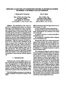
2.2

Percentage of articles per publisher in the studied universe of 84 papers. . . .

34

2.3

VMP Environment Taxonomy. Example references for each environment are presented. Unexplored environments are considered as Research Opportunities (RO). . . . . . . . . . . . . . . . . . . . . . . . . . . . . . . . . . . . . . . .

3.1

Example of placement in a virtualized datacenter infrastructure, composed by PMs, VMs and a network topology. . . . . . . . . . . . . . . . . . . . . . . .

3.2

61

Summary of results obtained in Experiment 2 using restricted lower and upper bounds against unrestricted bounds.

4.1

36

. . . . . . . . . . . . . . . . . . . . . .

79

Workload for Experiment 4 (10x100.vmp): number of running VMs as a function of time t. . . . . . . . . . . . . . . . . . . . . . . . . . . . . . . . . . . . 102

4.2

Workload for Experiment 4 (100x1000.vmp): number of running VMs as a function of time t. . . . . . . . . . . . . . . . . . . . . . . . . . . . . . . . . . 102

5.1

Experimental Workload Traces: Number of created VMs as a function of time t.118

6.1

Two-phase optimization scheme for VMP problems considered in this work, presenting a basic example with a placement recalculation time of β = 2 (from t = 2 to t = 4) and a placement reconfiguration time of γ = 1 (from t = 4 to t = 5). . . . . . . . . . . . . . . . . . . . . . . . . . . . . . . . . . . . . . . . 130

6.2

Temporal average cost: Average values of fs (x, t) in DC1 to DC5 per each scenario s ∈ S. . . . . . . . . . . . . . . . . . . . . . . . . . . . . . . . . . . 167

10

List of Tables 2.1

VMP Formulation Taxonomy. Example references for each environment are presented. Unexplored environments are considered as Research Opportunities (RO). In this table f1 (x): Energy Consumption, f2 (x): Network Traffic, f3 (x): Economical Costs, f4 (x): Performance, f5 (x): Resource Utilization. . . . . .

40

2.2

Objective Functions - Energy Consumption Minimization Group.

. . . . . .

44

2.3

Objective Functions - Network Traffic Minimization Group. . . . . . . . . . .

46

2.4

Objective Functions - Economical Costs Optimization Group. . . . . . . . .

47

2.5

Objective Functions - Performance Maximization Group. . . . . . . . . . . .

48

2.6

Objective Functions - Resource Utilization Maximization Group. . . . . . . .

48

2.7

Solution Techniques - Deterministic Algorithms . . . . . . . . . . . . . . . .

49

2.8

Solution Techniques - Heuristics . . . . . . . . . . . . . . . . . . . . . . . . .

50

2.9

Solution Techniques - Meta-Heuristics . . . . . . . . . . . . . . . . . . . . . .

51

2.10 Virtual Machine Placement Taxonomy. Elements of column % represent the percentage of articles in the studied universe [93]. For simplicity, MAM and PMO consider only the number of considered objective functions in column f (x). . . . . . . . . . . . . . . . . . . . . . . . . . . . . . . . . . . . . . . . .

52

3.1

Data of network links used in basic example (see Section 3.2.5). . . . . . . .

69

3.2

Types of PMs considered in experiments. For notation see Equation (3.4). .

76

3.3

Instance types of VMs considered in experiments. For notation see Equation (3.5). . . . . . . . . . . . . . . . . . . . . . . . . . . . . . . . . . . . . . . . .

3.4

77

Problem instances considered in Experiments 1 to 3, all with 50% of VMs with SLA s = 2. . . . . . . . . . . . . . . . . . . . . . . . . . . . . . . . . . .

77

3.5

Summary of results obtained by the proposed algorithm in Experiment 1. . .

78

3.6

Summary of results obtained by the proposed algorithm in Experiment 3. . .

81

11

4.1

Hardware configuration of PM types considered in Experiment 4. . . . . . .

99

4.2

Instance types of VMs considered. For notation see Equation (4.3). . . . . .

99

4.3

Number of non-dominated solutions per selection strategy. . . . . . . . . . . 100

4.4

Details of Experiment 4. . . . . . . . . . . . . . . . . . . . . . . . . . . . . . 100

4.5

Selection Strategy Comparison. For selection strategy notation see Section 4.3.103

5.1

Considered Data for Generated Experimental Workload Traces (W1 to W4 ). Details in [112]. . . . . . . . . . . . . . . . . . . . . . . . . . . . . . . . . . . 119

5.2

Objective Function Costs of Evaluated Algorithms. . . . . . . . . . . . . . . 120

5.3

Objective Function Costs of Evaluated Heuristics. . . . . . . . . . . . . . . . 121

5.4

VMs Migration Overhead for MA (A6). . . . . . . . . . . . . . . . . . . . . . 124

6.1

Summary of IaaS environments and VMPr methods already studied in related works. N/A indicates a Not Applicable criterion. . . . . . . . . . . . . . . . 133

6.2

Summary of evaluated algorithms as well as their corresponding VMPr Triggering and Recovering methods. N/A indicates a Not Applicable criterion. . 151

6.3

Basic example of how the proposed VMPr Triggering method predicts values ˆ = 3) based on previous discrete of F (x, t) for t = 16, t = 17 and t = 18 (N time instants, using Equation (6.23) with α = τ = 0.5. Predicted values are highlighted. . . . . . . . . . . . . . . . . . . . . . . . . . . . . . . . . . . . . 159

6.4

Types of PMs considered in simulations. For notation see Section 6.3. . . . . 161

6.5

Number of PMs per type on each considered IaaS cloud datacenter. . . . . . 162

6.6

Virtual Machine (VM) types from Amazon EC2 considered for cloud service requests in simulations. For notation see Section 6.3. . . . . . . . . . . . . . 162

6.7

Most relevant inputs for example workload trace presented in Table 6.8. . . . 163

6.8

Example of workload trace for a complex IaaS environment. For notation see Section 6.3. . . . . . . . . . . . . . . . . . . . . . . . . . . . . . . . . . . . . 164

6.9

Summary of evaluation criteria in experimental results for evaluated algorithms.165

List of Algorithms 1

Interactive Memetic Algorithm . . . . . . . . . . . . . . . . . . . . . . . . . .

72

2

Part 2 - Feasibility Verification . . . . . . . . . . . . . . . . . . . . . . . . . .

73

3

Part 2 - Infeasible Solutions Reparation . . . . . . . . . . . . . . . . . . . . .

74

4

Part 2 - Local Search

. . . . . . . . . . . . . . . . . . . . . . . . . . . . . . .

74

5

Extended Memetic Algorithm . . . . . . . . . . . . . . . . . . . . . . . . . . .

92

6

Part 3 - Feasibility Verification . . . . . . . . . . . . . . . . . . . . . . . . . .

94

7

Part 3 - Infeasible Solutions Reparation . . . . . . . . . . . . . . . . . . . . .

95

8

Part 3 - Local Search

96

9

First-Fit Decreasing (FFD) for iVMP. . . . . . . . . . . . . . . . . . . . . . . 154

10

Memetic Algorithm (MA) for VMPr. . . . . . . . . . . . . . . . . . . . . . . . 155

11

Minimum Migration Time (MMT) for VMPr running at PM Hi . . . . . . . . 156

12

Update-based VMPr Recovering. . . . . . . . . . . . . . . . . . . . . . . . . . 160

. . . . . . . . . . . . . . . . . . . . . . . . . . . . . . .

13

List of Acronyms ACO

Ant Colony Optimization

AUT

Adaptive Utilization Threshold

BF

Best-Fit

BFD

Best-Fit Decreasing

BIP

Binary Integer Programming

BSP

Backward Speculative Placement

CP

Constraint Programming

CPU

Central Process Unit

CRB

Cloud Resource Brokerage

CS

Cut-and-Search

CSB

Cloud Service Broker

CSP

Cloud Service Provider

CST

Cloud Service Tenant

CWTG

Cloud Workload Trace Generator

DES

Double Exponential Smoothing

DNS

Domain Name Service

DP

Dynamic Programming

DRF

Dominant Resource First

DVMA

Dynamic VM Allocation

EA

Evolutionary Algorithm

EC2

Elastic Compute Cloud

ECU

Elastic Compute Unit

ESA

Exhaustive Search Algorithm

FCFS

First-Come First-Served

FF

First-Fit

FFD

First-Fit Decreasing

GA

Genetic Algorithm

GPU

Graphical Process Unit

HF

Heaviest-Fit

IaaS

Infrastructure as a Service

ILP

Integer Linear Programming

IMSPM

Improved Multidimensional Space Partition Model

iVMP

Incremental Virtual Machine Placement

LMABBS

Live Migration Algorithm Based on a Basic Set

LP

Linear Programming

MA

Memetic Algorithm

MAc

Management Actions

MAM

Multi-Objective Problem solved as Mono-Objective

MaOP

Many-Objective Optimization Problem

MaVMP

Many-Objective Virtual Machine Placement

MBFD

Modified Best-Fit Decreasing

MBVMP

Migration-Based Virtual Machine Placement

MF

Main Finding

MILP

Mixed Integer Linear Programming

MIPS

Millions of Instructions per Second

MOEA

Multi-Objective Evolutionary Algorithm

MOP

Mono-Objective Optimization Problem

MVMP

Multi-Objective Virtual Machine Placement

NIC

Network Interface Card

NS

Neighborhood Search

P2P

Peer-to-Peer

PaaS

Platform as a Service

PBO

Pseudo-Boolean Optimization

PDF

Probability Distribution Function

PM

Physical Machine

PMO

Pure Multi-Objective Optimization Problem

PSO

Particle Swarm Optimization

QoE

Quality of Experience

QoS

Quality of Service

RO

Research Opportunity

SA

Simulated Annealing

SaaS

Software as a Service

SARMS

Self-Adaptive Resource Management System

SDN

Software Defined Networking

SIP

Stochastic Integer Programming

SLA

Service Level Agreement

SLLC

Shared Last Level Cache

SSD

Solid State Drive

TPOVMP

Two-Phase Online Virtual Machine Placement

TS

Tabu Search

VM

Virtual Machine

VMA

Virtual Machine Allocation

VMC

Virtual Machine Consolidation

VMcP

Virtual Machine Placement Consolidation

VMP

Virtual Machine Placement

VMPBBO

Virtual Machine Placement Biogeography-Based Optimization

VMPr

Virtual Machine Placement Reconfiguration

WAN

Wide Area Network

WF

Worst-Fit

Nomenclature

α

Smoothing factor, where 0 ≤ α ≤ 1.

∆rk,j (t)

Ratio of unsatisfied resource k at instant t where ∆rk,j (t) = 1 means no unsatisfied resource, while ∆rk,j (t) = 0 means resource k is unsatisfied.

λk

Protection factor for V rk,j ∈ [0,1]. Note that λk = 0 means full overbooking while λk = 1 means no-overbooking.

φk

Penalty factor for resource k, where φk ≥ 1.

τ

Trend factor, where 0 ≤ τ ≤ 1.

a

Network link identifier.

b

Number of constraints.

bt

Trend of F (x, t) at discrete time t.

C

Set of chromosomes.

ci

Datacenter identifier of Hi , where 1 ≤ ci ≤ cmax .

Cˆ

Constant, large enough to prioritize services with larger SLA over the ones with lower SLA.

Cla

Channel capacity of link la .

Dj,k

Binary variable that equals 1 if Vj and Vk are located in different PMs; otherwise, it is 0.

Dj,k (t)

Binary variable that equals 1 if Vj and Vk are located in different PMs at instant t. otherwise, it is 0.

fi (x, t)

Cost of original objective function fi (x, t).

fi (x, t)max

Maximum possible cost for fi (x, t).

fi (x, t)min

Minimum possible cost for fi (x, t).

fˆi (x, t)

Normalized cost of objective function fi (x, t) at instant t.

F (x, t)

Single objective function combining each fˆi (x, t) at instant t.

fs (x, t)

Combined objective function for all discrete time instants t in scenario s ∈ S.

fs (x, t)

Temporal average of combined objective function for all discrete time instants t in scenario s ∈ S.

F1

Average fs (x, t) for all scenarios s ∈ S [4].

F2

Maximum fs (x, t) considering all scenarios s ∈ S [4].

F3

Minimum fs (x, t) considering all scenarios s ∈ S.

Fa,i,i0

Binary variable that equals 1 if la ∈ mii0 ; otherwise, it is 0.

G

Network topology.

H

Set of available PMs.

Hi

PM with identifier i.

Hcpui

Processing resources of Hi .

Hhddi

Storage resources of Hi .

Hrami

Memory resources of Hi .

i

PM identifier.

j

VM identifier.

K

Capacity set of the communication channels.

L

Set of links in G.

Lz

Lower bound of objective function z.

la

Link with identifier a in L.

M

Set of paths for all-to-all PM interconnections.

m

Number of VMs.

mi,i0

Network path from Hi to Hi0 in M .

M Ac(Vj )

∈ Management actions that a hypervisor must execute in order to accommo-

{0, 1, 2, 3}

date the x(t + 1) placement corresponding to Vj .

M Ti,i0

Total amount of RAM memory to be migrated from PM Hi to Hi0 .

N

Size of the searching universe.

n

Number of PMs.

ˆ N

Number of prediction used in the proposed VMPr Triggering method.

P∗

Optimal Pareto set.

Pknown

Pareto set approximation.

Pt

Evolutionary population.

PF∗

Optimal Pareto front.

P Fknown

Pareto front approximation.

P Freduced

Reduced set of Pareto solutions.

P rk,i

Physical resource k on Hi , where 1 ≤ k ≤ r.

p

Number of decision variables.

pmaxi

Maximum power consumption of Hi .

pmini

Minimum power consumption of Hi . In what follows, pmini = pmaxi ∗0.6.

q

Number of objective functions.

Qt

Offspring population.

r

Number of considered resources.

Rj

Economical revenue for locating Vj .

Rj (t)

Economical revenue for allocating Vj in [$].

Rrk,j (t)

Economical revenue for attending V rk,j (t).

s

Highest priority level of SLAs.

St

Expected value of F (x, t) at discrete time t.

SLAj

Service Level Agreement SLAj of a Vj . If the highest priority level is s, then SLAj ∈ {1, . . . , s}.

T

Set of network communication between VMs.

T (t)

Set of network communication between VMs at instant t.

Tj,k

Average network traffic between Vj and Vk [Mbps]. Note that we can consider Tj,j = 0.

T la

Total amount of traffic going through link la [Mbps].

tmax

Duration of a scenario in discrete time instants.

u

Feasible solution.

U

Set of decision vectors.

Uz

Upper bound of objective function z.

U cpui

Utilization ratio of processing resources used by Hi .

U rk,i (t)

Utilization ratio of resource k of PM Hi at instant t.

V

Set of requested VMs.

V (t)

Set of requested VMs at instant t.

V cpuj

Processing requirements of Vj .

V hddj

Storage requirements of Vj .

V ramj

Memory requirements of Vj .

V rk,j (t)

Virtual resource k on Vj , where 1 ≤ k ≤ r.

Vj

VM with identifier j.

v

Feasible solution.

wi

Weight of importance associated to fi (x).

x

Placement matrix / solution.

X

Decision space.

Xf

Feasible decision space.

Xj

Binary variable that equals 1 if Vj is located for execution on any PM; otherwise, it is 0.

Xj (t) ∈ {0, 1}

Indicates if Vj is allocated for execution on a PM (Xj (t) = 1) or not (Xj (t) = 0) at instant t.

Xˆj

Indicates if Vj is allocated on the main provider (Xˆj = 0) or on an alternative datacenter of the cloud federation (Xˆj = 0.7).

xj,i

Binary variable equals 1 if Vj is located to run on Hi ; otherwise, it is 0.

xj,i (t) ∈ {0, 1}

Indicates if Vj is allocated (xj,i (t) = 1) or not (xj,i (t) = 0) for execution in a PM Hi (i.e., xj,i (t) : Vj → Hi ) at a discrete time t.

y

Objective vector.

Y

Objective space.

Yi

Binary variable equals 1 if Hi is turned on; otherwise, it is 0.

Yi (t) ∈ {0, 1}

Indicates if Hi is turned on (Yi (t) = 1) or not (Yi (t) = 0) at instant t.

Yf

Feasible objective space.

z

Objective function identifier.

Zt

Known value of F (x, t) at discrete time t.

Z t+1

Value of F (x, t + 1) predicted at discrete time t.

Zj (t)

Binary variable that equals 1 if M A(Vj ) = 2, i.e. Vj is migrated, otherwise, it is 0 (Vj is not migrated).

21

1

Introduction

A significant number of research challenges for delivering computational resources as an utility (like water, electricity, gas, and telephony) has already been identified [19]. In this context, cloud computing datacenters deliver infrastructure (IaaS), platform (PaaS) and software (SaaS) as services, available to end users in a pay-as-you-go basis [107]. Achieving an efficient resource management for IaaS service model in cloud computing datacenters could be considered one of the most relevant challenges, including important research topics such as: resource allocation, resource provisioning, resource mapping and resource adaptation [104]. Admission control and proactive elasticity could be also considered relevant research topics related to resource management in cloud computing datacenters [40]. The present work focuses on resource allocation, specifically in one of the most studied problems for resource allocation in cloud computing datacenters: the process of selecting which virtual machines (VMs) should be hosted at each physical machine (PM) of a cloud computing infrastructure, commonly known as Virtual Machine Placement (VMP) problem. Several research articles in the specialized literature demonstrated that solving the VMP problem for efficient allocation of resources in cloud computing datacenters could significantly improve energy-efficiency, quality of service (QoS), carbon dioxide emissions, among other advantages; all of them with significant economical [6, 18] and ecological impact [13, 18]. Beloglazov and Buyya proposed in [14] four different sub-problems for resource allocation in cloud datacenters: (1) determining when a PM is overloaded, requiring migration of VMs from this PM; (2) determining when a PM is underloaded, requiring migration of all VMs from this PM and switching the PM to sleep mode; (3) selecting VMs to migrate from an overloaded PM; and (4) finding a new placement of the VMs selected for migration, considering overloaded and underloaded PMs. A conceptual architecture considering the most studied problems related to resource allocation in cloud computing datacenters is presented in [40], where placement of admitted services (composed by VMs) could be solved considering different criteria and requirements. 22

In cloud computing datacenters, there are several criteria that can be considered when selecting a possible solution for a VMP problem, depending on management policies and optimization objectives. These criteria can even change from one period of time to another, which implies a variety of possible environments, formulations and different objectives to be considered for optimization of the VMP problem. In this context, nearly 60 different objective functions were identified in the VMP literature [93, 94, 96]. Taking into account the large number of existing objective functions and possible approaches for objective function modeling, providers of cloud computing datacenters must be able to formulate the VMP problem as a Pure Multi-Objective Optimization Problem (PMO), optimizing more than just one objective function at a time (e.g. achieve economical revenue maximization by simultaneously minimizing the total economical penalties for SLA violations, minimizing operational costs and maximizing the profit for leasing resources). It is important to consider that PMOs simultaneously optimizing more than three objective functions are known as Many-Objective Optimization Problems (MaOPs), as defined in [27]. Several challenges should be considered when solving problems with more than three objective functions [45]. These challenges are intrinsically related to the fact that as the number of objective functions increase, the proportion of non-dominated solutions in the population grows, being increasingly difficult to discriminate among solutions using only the Pareto dominance relation [32]. Additionally, determining which solution to keep and which to discard in order to converge toward the Pareto set is still a relevant issue to be addressed [45], making more difficult to solve MaOPs. Clearly, existing difficulties in solving MaOPs explain why it is still considered an unexplored domain in resource management of cloud computing datacenters [58] and no many-objective formulations have already been proposed for the VMP problem in the specialized literature before this doctoral thesis [94, 96]. The main scope of this doctoral thesis is Many-Objective Virtual Machine Placement (MaVMP) from the perspective of cloud computing providers, focusing on single-cloud deployments for the following formulations of MaVMP problems: (1) initial placement of VMs (static), (2) reconfiguration of VMs (semi-dynamic), and (3) for cloud computing (dynamic).

23

1.1

Research Problems and Objectives

This doctoral thesis tackles research challenges in relation to Many-Objective Virtual Machine Placement (MaVMP) problems for virtualized datacenters and cloud computing environments. In particular, the following research problems are investigated: 1. How to formulate and solve MaVMP problems: The number of objective functions may be rapidly increased once a complete understanding of the VMP problem is accomplished for practical problems, where many different parameters should be considered [96]. Based on the large number of possible objective functions for the VMP, this problem can clearly be addressed as a Many-Objective Virtual Machine Placement (MaVMP). Considered MaVMP formulations include: (1) initial placement (static), (2) reconfiguration of VMs (semi-dynamic), and (3) for cloud computing (dynamic). 2. How to manage solutions for a MaVMP problem: As the number of conflicting objectives of a MaVMP problem formulation increases, the total number of nondominated solutions increases (even exponentially in some cases), being increasingly difficult to discriminate among solutions using only the Pareto dominance relation [32]. Proposing methods to effectively reduce the number of solutions in a MaVMP problem for initial placement of VMs can be considered a relevant research challenge. 3. How to select solutions for a MaVMP problem: In a pure multi-objective context, a Pareto set approximation can be composed by a large number of nondominated solutions [143]. Automatically selecting the most convenient solution from a set of non-dominated solutions can also be considered as a research challenge for solving MaVMP problems with reconfiguration of VMs. 4. How to model MaVMP problems for cloud computing under uncertainty: In cloud computing environments, particularly for IaaS service model, several parameters could be considered as uncertain variables, taking into account its on-demand provisioning model. Cloud computing datacenter managers should be able to effectively deal with uncertain parameters for MaVMP problems. 24

To deal with the research challenges associated to the above mentioned research problems, the following objectives have been delineated: 1. Explore, analyze, and classify research of the Virtual Machine Placement (VMP) problem to gain a systematic understanding of the existing approaches and formulations. 2. Formulate for the first time the following resource allocation problems: (a) MaVMP for initial placement of VMs (static); (b) MaVMP with reconfiguration of VMs (semi-dynamic); (c) MaVMP for cloud computing under uncertainty (dynamic). 3. Provide an effective method for reducing the potentially unmanageable number of nondominated solutions in the MaVMP problem for initial placement of VMs in virtualized datacenters. 4. Develop an algorithm specially designed for solving MaVMP problems for initial placement of VMs in virtualized datacenters. 5. Evaluate strategies for automatically selecting a convenient solution from a Pareto set approximation for MaVMP problems with reconfiguration of VMs. 6. Extend the algorithm proposed in item 4, firstly designed for solving MaVMP problems for initial placement of VMs, to solve MaVMP problems with reconfiguration of VMs. 7. Propose a complex IaaS environment for VMP problems considering the most relevant dynamic parameters in the specialized literature. 8. Propose and experimentally evaluate novel methods related to the resolution of VMP problems in uncertain cloud computing environments.

1.2

Contributions

The main contributions of this doctoral thesis are directly related to each of the delineated objectives. The key contributions are: 25

1. Taxonomies of VMP problems for cloud computing (Objective 1) [10, 94, 96]. 2. First formulations of the following resource allocation problems: (a) A general many-objective optimization framework that is able to consider as many objective functions as needed when formulating MaVMP problems for initial placement in virtualized datacenters. As a utilization example of the proposed framework, for the first time a formulation of a MaVMP for initial placement was proposed, considering the simultaneous optimization of the following objective functions: (1) power consumption, (2) network traffic, (3) economical revenue, (4) quality of service and (5) network load balancing (Objective 2(a)) [92, 95]. (b) A formulation of a MaVMP problem with reconfiguration of VMs considering the simultaneous optimization of the following five conflicting objective functions: (1) power consumption, (2) inter-VM network traffic, (3) economical revenue, (4) number of VM migrations and (5) network traffic overhead for VM migrations (Objective 2(b)) [68]. (c) A formulation of a MaVMP problem for cloud computing environments, optimizing the following four objective functions: (1) power consumption, (2) economical revenue, (3) resource utilization and (4) placement reconfiguration time. Additionally, a first scenario-based uncertainty approach for modeling the following relevant uncertain parameters of a proposed complex IaaS environment: (1) virtual resources capacities (vertical elasticity), (2) number of VMs that compose cloud services (horizontal elasticity), (3) utilization of CPU and RAM memory virtual resources (relevant for overbooking) as well as (4) utilization of networking virtual resources (also relevant for overbooking) (Objective 2(c)) [99]. 3. A method for reducing the potentially unmanageable number of non-dominated solutions for MaVMP problems for initial placement in virtualized datacenters. The proposed method is based on adjustable lower and upper bounds associated to each objective function. The effectiveness of the proposed method converging to a manageable number of solutions was proved in different experiments (Objective 3) [92, 95]. 26

4. An interactive Memetic Algorithm (MA), designed for solving MaVMP problems for initial placement of VMs in virtualized datacenters. An experimental evaluation of the quality of solutions obtained by the proposed algorithm against optimal solutions in different scenarios as well as its scalability solving instances of the problem with large numbers of PMs and VMs (Objective 4) [95]. 5. An experimental evaluation of strategies for automatically selecting a convenient solution from a Pareto set approximation for MaVMP problems with reconfiguration of VMs. The following five selection methods were evaluate in different scenarios: (1) random, (2) preferred solution, (3) minimum distance to origin, (4) lexicographic order for providers and (5) lexicographic order for service (Objective 5) [68]. 6. An extended MA for solving MaVMP problems with reconfiguration of VMs, including the implementation of five evaluated selection strategies (Objective 6) [68]. 7. A first proposal of a complex IaaS environment for VMP problems considering service elasticity, including both vertical and horizontal scaling of cloud services and overbooking of physical resources, including server (CPU and RAM) as well as networking resources (Objective 7) [99]. 8. A two-phase optimization scheme for VMP problems, combining advantages of both online (iVMP) and offline (VMPr) VMP formulations in the proposed IaaS environment, introducing a novel prediction-based VMPr Triggering method to decide when to trigger a placement reconfiguration as well as a novel update-based VMPr Recovering method to decide what to do with VMs requested during placement recalculation times (Objective 8) [99].

1.3

Thesis Organization

The core parts and chapters of this doctoral thesis are derived from articles published during the doctoral candidature. The remainder of this doctoral thesis is organized as follows:

27

• Part I presents taxonomies of the VMP problem for cloud computing datacenters, presenting a general vision of the mentioned problem and identifying main research opportunities. This chapter is derived from: – Fabio López-Pires and Benjamín Barán (2015), ‘A Virtual Machine Placement Taxonomy’. In 2015 15th IEEE/ACM International Symposium on Cluster, Cloud and Grid Computing (CCGrid), (pp. 159-168), China. IEEE [94]. – Fabio López-Pires and Benjamín Barán (2017), ‘Cloud Computing Resource Allocation Taxonomies’. International Journal of Cloud Computing. Inderscience Publishers [96]. – Benjamín Barán and Fabio López-Pires (2017), ‘Resource Allocation for Cloud Infrastructures: Taxonomies and Research Challenges’. Research Advances in Cloud Computing. S. Chaudhary, G. Somani, R. Buyya (Editors). Springer [10]. • Part II proposes a general many-objective optimization framework for MaVMP problems for initial placement of VMs, including a method for effectively reducing the potentially unmanageable number of non-dominated solutions as well as an interactive MA for solving the formulated problems. This chapter is derived from: – Fabio López-Pires and Benjamín Barán (2015), ‘A Many-Objective Optimization Framework for Virtualized Datacenters’. In 2015 5th International Conference on Cloud Computing and Service Science (CLOSER), (pp. 439-450), Portugal. SciTePress (Best Student Paper Award) [92]. – Fabio López-Pires and Benjamín Barán (2017), ‘Many-Objective Virtual Machine Placement’. Journal of Grid Computing. Springer (Invited Paper) [95]. • Part III presents a first formulation of a MaVMP problem with reconfiguration of VMs, considering the simultaneous optimization of five objective functions. Additionally, an evaluation of five different strategies for automatically selecting a convenient solution from a Pareto set approximation as well as an extended MA for solving the formulated problem are also presented. This chapter is derived from:

28

– Diego Ihara, Fabio López-Pires and Benjamín Barán (2015), ‘Many-Objective Virtual Machine Placement for Dynamic Environments’. In 2015 IEEE/ACM 8th International Conference on Utility and Cloud Computing (UCC), (pp 203-207), Cyprus. ACM/IEEE [68]. – Fabio López-Pires (2016), ‘Many-Objective Resource Allocation in Cloud Computing Datacenters". 4th IEEE International Conference on Cloud Engineering (IC2E). Doctoral Symposium. Germany. IEEE [88]. – Fabio López-Pires and Benjamín Barán (2017), ‘Many-Objective Optimization for Virtual Machine Placement in Cloud Computing’. Research Advances in Cloud Computing. S. Chaudhary, G. Somani, R. Buyya (Editors). Springer [97]. • Part IV presents a first formulation of a MaVMP problem for cloud computing considering the optimization of four objective functions in a complex IaaS environment. Additionally, a first scenario-based uncertainty approach for modeling four uncertain parameters of the proposed complex IaaS environment is presented, as well as novel methods related to the resolution of the proposed problem in cloud computing datacenters. This chapter is derived from:. – Fabio López-Pires, Benjamín Barán, Augusto Amarilla, Leonardo Benítez, Rodrigo Ferreira, Saúl Zalimben (2016), ‘An Experimental Comparison of Algorithms for Virtual Machine Placement Considering Many Objectives". 9th IFIP Latin America Networking Conference (LANC). Chile. ACM [98]. – Fabio López-Pires, Benjamín Barán, Leonardo Benítez, Saúl Zalimben, Augusto Amarilla (Under Review), ‘Virtual Machine Placement for Elastic Infrastructures in Overbooked Cloud Computing Datacenters Under Uncertainty". Future Generation Computer Systems. Elsevier [99]. • Part V summarizes the main findings of this doctoral thesis and presents several future research directions.

29

1.4

Additional Publications

• Publications by the author in related research topics not included in this thesis: – Sara Arévalos, Fabio López-Pires, Benjamín Barán (2015), ‘Auction-based Resource Provisioning in Cloud Computing. A Taxonomy’. In XLI Latin American Computing Conference (CLEI), Perú. IEEE [8]. – Jammily Ortigoza, Fabio López-Pires, Benjamín Barán (2016), ‘A Taxonomy on Dynamic Environments for Provider-oriented Virtual Machine Placement". In 4th International Conference on Cloud Engineering (IC2E). Germany. IEEE [112]. – Sara Arévalos, Fabio López-Pires, Benjamín Barán (2016), ‘Comparative Evaluation of Algorithms for Auction-based Cloud Pricing Prediction". In 4th IEEE International Conference on Cloud Engineering (IC2E). Germany. IEEE [7]. – Lino Chamorro, Fabio López-Pires, Benjamín Barán (2016), ‘A Genetic Algorithm for Dynamic Cloud Application Brokering". In 4th International Conference on Cloud Engineering (IC2E). Germany. IEEE [24]. – Jammily Ortigoza, Fabio López-Pires, Benjamín Barán (2016), ‘Workload Generation for Virtual Machine Placement in Cloud Computing Environments". In XLII Latin American Computing Conference (CLEI). Chile. IEEE [113]. – Augusto Amarilla, Leonardo Benítez, Saúl Zalimben, Fabio López-Pires, Benjamín Barán (2017), ‘Evaluating a Two-Phase Virtual Machine Placement Optimization Scheme for Cloud Computing Datacenters". In 12th Metaheuristics International Conference (MIC). Spain. [5]. – Nabil Chamas, Fabio López-Pires, Benjamín Barán (2017), ‘Two-Phase Virtual Machine Placement Algorithms for Cloud Computing. An Experimental Evaluation under Uncertainty". Accepted at XLIII Latin American Computing Conference (CLEI). Argentina.

30

Part I Literature Review

31

2

VMP Taxonomies for Cloud Computing

The VMP problem has been extensively studied in cloud computing literature and several surveys have already been presented. Existing surveys focused on specific issues such as: (1) energy-efficient techniques applied to the problem [13, 120], (2) particular deployment architectures where the VMP problem is applied, as federated clouds [50], and (3) methods for comparing performance of placement algorithms in large on-demand clouds [109]. The above mentioned surveys and research articles focused into specific issues related to the VMP problem. Consequently, López-Pires and Barán proposed in [94, 96] a general and extensive study of a large part of the VMP literature including 84 studied articles [93], presenting a wide analysis of the existing approaches for the formulation and resolution of the VMP as an optimization problem. Additionally, a novel taxonomy was proposed in [94] for the classification of the studied articles by the main following criteria: (1) optimization approach, (2) objective function and (3) solution technique. The taxonomy presented in [94] was extended, including novel taxonomies and presenting a detailed view of the existing approaches as well as several possible research opportunities to further advance in this research area. The presented taxonomies [96] could guide interested readers to: (1) understand different possible environments where a VMP problem could be studied, considering both provider and broker perspectives in different deployment architectures, (2) identify existing approaches for the formulation and resolution of the VMP as an optimization problem and (3) present a detailed view of the VMP problem, identifying research opportunities to further advance in this research area.

2.1

VMP Literature Review

For this doctoral thesis, a selection process of current research was defined and performed in order to study a large part of the most relevant VMP literature. This section presents a detailed description of the literature selection process which is summarized in Figure 2.1. 32

keyword search

publisher filtering

abstract reading

selected articles

(446 articles)

(172 articles)

(93 articles)

(84 articles)

Figure 2.1: VMP literature selection process.

2.1.1

Keywords Search

The selection process of relevant articles started with a search of research articles from Google Scholar database [scholar.google.com] with at least one of the following selected keywords in the article title: (1) virtual machine placement, (2) vm placement, (3) virtual machine consolidation, (4) vm consolidation or (5) server consolidation. This keywords search step results in 446 research articles. A detailed list of the 446 resulting articles could be found in [91], specifically in the worksheet keywords search.

2.1.2

Publisher Filtering

Considering the large number of results from keywords search step, the literature selection process focused in research articles published by the following relevant publishers: (1) ACM, (2) IEEE, (3) Elsevier and (4) Springer. Percentage of articles per publisher in the studied universe is summarized in Figure 2.2. This publisher filtering step results in a reduction from 446 to 172 (38.6%) research articles of the literature. A detailed list of the 172 resulting articles could be found in [91], specifically in the worksheet publisher filtering.

2.1.3

Reading of Abstract

Considering the 172 resulting articles from the previous step, a reading of the abstract was performed to identify only the most relevant articles that study the VMP problem. 33

ACM

IEEE 11% 69% 5%

Elsevier 15% Springer Figure 2.2: Percentage of articles per publisher in the studied universe of 84 papers. After the reading of the abstract, 93 research articles were selected from the VMP literature. A detailed list of the 93 resulting articles could be found in [91], specifically in the worksheet abstract reading. Finally, short papers (i.e. research articles with less than 6 pages) were removed from the selected literature, resulting in 84 selected articles of the VMP literature for the detailed study presented in this doctoral thesis.

2.2

VMP Environment Taxonomy

Depending on the particular environment where a VMP problem will be studied, several different considerations should be taken into account before considering a particular formulation or technique for the resolution of the considered VMP problem. In this context, different possible environments could be identified by classifying research articles in the VMP literature by: (1) orientation, (2) deployment architecture and (3) type of formulation. First, a VMP problem could be studied from both provider or broker perspectives. A provider-oriented VMP problem could be studied considering one of the following deployment architectures: single-cloud, distributed-cloud or federated-cloud, while a broker-oriented VMP problem could be studied considering a multi-cloud deployment architecture. Additionally, both provider-oriented and broker-oriented VMP problems, in any of the possible deployment architectures, could be studied considering two different types of formulation: offline or online formulations. 34

For a complete understanding of the possible environments where a VMP problem could be studied, considering both provider and broker perspectives in different deployment architectures, Figure 2.3 presents the taxonomy described in this section including example references from the studied VMP literature [93]. The following subsections present a detailed description of the mentioned classification criteria, including important definitions for a complete understanding of the VMP problem.

2.2.1

Orientations: Provider-oriented or Broker-oriented

Definition 2.2.1 A provider-oriented VMP problem is the process of selecting which VMs should be hosted at each PMs of a cloud computing infrastructure. Resource allocation in cloud computing datacenters is a main concern for Cloud Service Providers (CSPs). According to [94], the VMP problem is mainly formulated from this perspective. It should be mentioned that in a provider-oriented VMP, a Cloud Service Tenant (CST) cannot decide which PMs will host the requested VMs. In the specialized literature, this particular problem is also known as Virtual Machine Allocation (VMA) problem [69]. Definition 2.2.2 A broker-oriented VMP problem is the process of selecting which VMs should be hosted at each Cloud Service Provider (CSP) of a cloud computing market. Considering that the number of CSPs has been rapidly increased and nowadays there are different pricing schemes, VM offers and features, it is difficult for CSTs to search for the most convenient option in cloud computing markets and decide which CSP is the most convenient to host the requested resources. Consequently, a VMP problem can also be formulated from a broker perspective who is responsible of helping CSTs to find good allocation deals. This particular problem is also known as Cloud Resource Brokerage (CRB) problem [140].

2.2.2

Deployment Architectures

Different deployment architectures can be considered for a VMP problem, depending on the number of cloud computing datacenters associated to the problem instance and the type of interconnection or relation of these datacenters. 35

VMP Problem Provider-oriented Single-Cloud Offline [89]

Distributed-Cloud

Online Offline [121]

Broker-oriented

[26]

Federated-Cloud

Online Offline [15]

RO

Multi-Cloud

Online

Offline

Online

[39]

[105]

RO

Figure 2.3: VMP Environment Taxonomy. Example references for each environment are presented. Unexplored environments are considered as Research Opportunities (RO). A provider-oriented VMP problem could be studied considering one of the following deployment architectures: single-cloud, distributed-cloud or federated-cloud, while a brokeroriented VMP problem could be studied in a multi-cloud deployment architecture. Definition 2.2.3 A provider-oriented VMP problem in a single-cloud deployment is the process of selecting which VMs should be hosted at each PMs of a single cloud datacenter. In scenarios considering a single cloud computing datacenter, a CSP could formulate a VMP problem subject to commonly studied constraints such as: unique placement of VMs, maximum capacity of resources [89] or Service Level Agreement (SLA) compliance [6, 65]. According to [94], the single-cloud deployment architecture is the most studied scenario. Definition 2.2.4 A provider-oriented VMP problem in a distributed-cloud deployment is the process of selecting which VMs should be hosted at each PMs of more than one cloud computing datacenter owned by the same Cloud Service Provider (CSP). For CSPs with a global infrastructure (e.g. Amazon), a single-cloud deployment architecture could be extended to several distributed cloud computing datacenters, where the formulation of a VMP problem may include particular constraints and considerations. CSPs with geo-distributed cloud computing datacenters may be interested in studying a VMP problem for the provision of differentiated services to world-wide tenants, such as redundancies of services (placement of VMs in different datacenters) [101] or quality and performance of services (placement of VMs in datacenters closer to end users) [17], increasing the complexity of the VMP problem formulation. 36

Definition 2.2.5 A provider-oriented VMP problem in a federated-cloud deployment is the process of selecting which VMs should be hosted at each PMs of more than one cloud computing datacenter owned by different Cloud Service Providers (CSPs) in a cloud federation. In federated clouds, CSPs with excess capacity lease resources to other CSPs in need of temporary additional resources; consequently, particular considerations associated to a VMP problem in this deployment architecture have to be studied [50]. For example, trading policies are generally not the same for CSPs that form part of the same cloud federation, so a VMP problem could be studied for cost-effective selection of CSPs for workload peaks. Definition 2.2.6 A broker-oriented VMP problem in a multi-cloud deployment is the process of selecting which VMs should be hosted at each Cloud Service Provider (CSP) of a cloud computing market composed by more than one CSP. Cloud Service Brokers (CSBs) or CSTs can require VMs to be deployed in cloud computing datacenters owned by different CSPs, according to particular requirements such as disaster recovery reasons or due to legislation [41], just to cite a few.

2.2.3

Types of Formulation: Offline or Online

A VMP problem could be formulated as an offline problem considering the placement of VMs into PMs (for provider-oriented VMP) or VMs into CSPs (for broker-oriented VMP) for a static or semi-dynamic cloud service deployment. Definition 2.2.7 An offline formulation of a provider-oriented VMP problem in any possible deployment architecture could be understood as the process of selecting which VMs should be hosted at each PMs of the considered cloud computing datacenters for a static or semi-dynamic cloud service deployment. For a provider-oriented VMP, an offline formulation considers a previously known set of VMs requested in static or semi-dynamic environments. It should be noted that offline formulations of VMP problems are mostly appropriate for initial placement of VMs [89, 92, 100]

37

or for virtualized datacenters with deployments of VMs that rarely change its configuration over time (i.e. reconfiguration of VMs) [68]. Definition 2.2.8 An offline formulation of a broker-oriented VMP problem could be understood as the process of selecting which VMs should be hosted at each CSP of the considered cloud computing market for a static cloud service deployment. The broker-oriented VMP is mostly formulated as an offline problem, considering that possible re-locations of VMs to different CSPs are still limited by interoperability factors. A VMP problem could also be formulated as an online problem considering the placement of VMs into PMs (provider-oriented VMP) or VMs into CSPs (broker-oriented VMP) for a cloud service deployment with dynamic demand or parameters that change over time. Definition 2.2.9 An online formulation of a provider-oriented VMP problem in any possible deployment architecture could be understood as the process of selecting which VMs should be hosted at each PMs of the considered cloud computing datacenters considering dynamic demand or parameters that change over time. It should be noted that an online formulation for a provider-oriented VMP problem could be a more appropriate approach for resource allocation in cloud computing datacenters, considering the on-demand model of cloud computing with dynamic resource provisioning and dynamic workloads of modern cloud applications [14]. In this context, preliminary results out of the scope of this work studied an extended taxonomy for the classification of possible online formulations for the provider-oriented VMP, presenting an analysis of possible challenges for providers in cloud computing environments based on the most relevant dynamic parameters studied so far in the existing VMP literature such as: (1) resource capacities of VMs (related to vertical elasticity), (2) number of VMs of a service (related to horizontal elasticity) and (3) utilization of resources of VMs (related to overbooking) [112]. It should be noted that extending the taxonomies presented in this work for specializing possible VMP environments could be considered as a research opportunity to further advance in this research area.

38

Definition 2.2.10 An online formulation of a broker-oriented VMP problem in any possible deployment architecture could be understood as the process of selecting which VMs should be hosted at each CSPs of a given cloud computing market considering demands or parameters that change over the time. Considering that the number of CSPs has been rapidly increased, nowadays several dynamic parameters could be considered for the broker-oriented VMP problem such as: (1) dynamic pricing schemes, (2) dynamic VM offers or (3) dynamic requirements. Research on online formulations of the broker-oriented VMP problem should advance to address existing opportunities in emerging cloud computing markets as presented in a few articles [82, 102].

2.3

VMP Formulation Taxonomy

Considering each possible environment where a VMP problem could be studied (see Figure 2.3), several different formulations of the problem could be proposed. In this context, formulations of a VMP problem may be classified by the: (1) optimization approach, (2) objective function and (3) solution technique, as initially considered in [94]. First, a VMP problem could be formulated considering one of the following optimization approaches: (1) mono-objective (MOP), (2) multi-objective solved as mono-objective (MAM) or (3) pure multi-objective (PMO). Once the optimization approach is defined, formulations may also be classified by the objective function(s) studied, both in minimization and maximization contexts. These objective functions could be optimized separately or simultaneously, depending on the selected optimization approach. Finally, solution techniques for solving a VMP problem could be used as a third classification criterion [94]. For a complete understanding of possible approaches for the formulation and resolution of a VMP problem, Table 2.1 presents the taxonomy described in this section, including example references from the studied VMP literature [93]. The following subsections present a detailed description of the classification criteria above defined as well as special considerations for particular formulations.

39

Table 2.1: VMP Formulation Taxonomy. Example references for each environment are presented. Unexplored environments are considered as Research Opportunities (RO). In this table f1 (x): Energy Consumption, f2 (x): Network Traffic, f3 (x): Economical Costs, f4 (x): Performance, f5 (x): Resource Utilization. Objective Functions Technique Approach f1 (x) f2 (x) f3 (x) f4 (x) f5 (x) MOP [53] [114] [30] [15] [84] Deterministic MAM [6, 131] [6, 129] RO RO [129, 131] Algorithms PMO RO RO RO RO RO MOP [39] [33] [125] [55] [84] Heuristics MAM [37, 121] [37, 61] [29, 61] [121, 146] [20, 21] PMO RO RO RO RO RO MOP [135] RO [105] [142] RO MetaMAM [26, 150] [26, 126] [1, 150] [126] [1, 150] Heuristics PMO [51, 89] [89, 100] [89, 100] RO [51] MOP [148] RO RO RO RO Approximation MAM [43] RO RO RO RO Algorithms PMO RO RO RO RO RO

2.3.1

Optimization Approaches

This section presents the optimization approaches considered in the articles studied in [94]. The identified optimization approaches may be classified as: (1) mono-objective (MOP), (2) multi-objective solved as mono-objective (MAM) and (3) pure multi-objective (PMO). The mentioned optimization approaches are detailed in the following subsections.

Mono-Objective (MOP) A mono-objective optimization approach (MOP) considers the optimization of one objective function or the individual optimization of more than one objective function, one at a time. Research on the VMP problem has been mainly guided by the MOP approach, identifying almost 40 different objective functions proposed considering this optimization approach [94]. It should be noted that an objective function could be studied considering different modeling approaches (e.g. economical revenue maximization could be achieved by minimizing the total economical penalties for SLA violations [30], by minimizing operational costs [65, 66] or even by maximizing the total profit for leasing resources [125]).

40

Multi-Objective solved as Mono-Objective (MAM) The optimization of multiple objective functions combined into one objective function is considered in this work as a multi-objective problem solved as mono-objective (MAM). This hybrid approach enables the optimization of multiple objectives functions with the disadvantage that it requires a deep knowledge of the problem domain to allow a correct combination of the objective functions, which in most cases is not possible [11]. A growing number of articles have proposed formulations of the VMP problem with this hybrid approach [93]. Different methods could be considered for a formulation of a VMP problem with a MAM approach such as: weighted sum, solving the problem as mono-objective while considering the other objective functions as constraints of the problem or even proposing fuzzy logic to provide an efficient way for combining conflicting objectives and expert knowledge [93].

Pure Multi-Objective (PMO) A general Pure Multi-Objective Optimization (PMO) problem includes a set of p decision variables, q objective functions, and b constraints. Objective functions and constraints are functions of decision variables. In a PMO formulation, x represents the decision vector (or solution), while y represents the objective vector (or solution cost). The decision space is denoted by X and the objective space as Y . These can be expressed as [28]: Optimize: y = f (x) = [f1 (x), f2 (x), ..., fq (x)]

(2.1)

e(x) = [e1 (x), e2 (x), ..., eb (x)] ≥ 0

(2.2)

x = [x1 , x2 , ..., xp ] ∈ X

(2.3)

y = [y1 , y2 , ..., yq ] ∈ Y

(2.4)

subject to:

where:

41

The set of constrains e(x) ≥ 0 defines the set of feasible solutions Xf ⊂ X and its corresponding set of feasible objective vectors Yf ⊂ Y . The feasible decision space Xf is the set of all decision vectors x in the decision space X that satisfies the constraints e(x) given by Equation (2.2). The feasible objective space Yf is the set of the objective vectors y that represents the image of Xf onto Y . These feasible spaces are defined as:

Xf = {x | x ∈ X ∧ e(x) ≥ 0}

(2.5)

Yf = {y | y = f (x) ∀x ∈ Xf }

(2.6)

To compare two solutions in a pure multi-objective context, the concept of Pareto dominance is used. Given two feasible solutions u, v ∈ Xf , u dominates v, denoted as u  v, if f (u) is better or equal to f (v) in every objective function and strictly better in at least one objective function. If neither u dominates v, nor v dominates u, u and v are said to be non-comparable (denoted as u ∼ v). A decision vector x is non-dominated with respect to a set U , if there is no member of U that dominates x. The set of non-dominated solutions of the whole set of feasible solutions Xf , is known as optimal Pareto set P ∗ . The corresponding set of objective vectors constitutes the optimal Pareto front P F ∗ . Taking into account the large number of existing objective functions and possible approaches for objective function modeling identified in [93, 94], PMO approaches could result in more realistic formulations of a VMP problem, optimizing more than just one objective function at a time (e.g. achieve economical revenue maximization by simultaneously minimizing the total economical penalties for SLA violations, minimizing operational costs and maximizing the profit for leasing resources). In this context, PMOs optimizing more than three objective functions are known as Many-Objective Optimization Problems (MaOPs), as defined in [27]. MaOPs differ significantly from PMOs because several issues should be considered when solving optimization problems with more than three objective functions [45]. In case of Pareto-based algorithms, these issues are intrinsically related to the fact that as the number of objective functions increases, the proportion of non-dominated solutions grows, being 42

increasingly difficult to discriminate among solutions using only the Pareto dominance relation [32]. Additionally, determining which solution to keep and which to discard in order to converge toward the Pareto set is still a relevant issue to be addressed [45]. As the number of objective functions grow, the proportion of non-dominated solutions to the total number of solutions tends to one [143], making more difficult to solve a MaOP.

2.3.2

Objective Function Groups

In cloud computing datacenters, there are several criteria that can be considered when selecting a possible solution for a VMP problem, depending on management policies and optimization objectives. These criteria can even change from one period of time to another, which implies a variety of possible formulations of the problem and different objectives to be optimized. According to [94], the VMP literature mainly focuses on the optimization of objective functions that specifically concerns CSPs (provider-oriented VMP). Objective functions could also be formulated considering the requirements of CSTs for allocation of a particular service or application, often composed by more than one VM (broker-oriented VMP). It should be mentioned that in [94], nearly 60 different objective functions were identified for the three optimization approaches presented in Section 2.3.1. Considering the large number of proposed objective functions, identified objective functions with similar characteristics and goals were classified into 5 objective function groups that are presented in the following subsections (see Tables 2.2 to 2.6). Additionally, considering that MAM and PMO optimization approaches may take into account any combination of each objective function group or even different objective functions from the same objective function group, a simplified classification is considered in this work (see Tables 2.1 and 2.10).

f1 (x) - Energy Consumption Energy consumption management is an important studied issue in the provider-oriented VMP literature, with high impact in operational costs and carbon dioxide emissions for cloud datacenter operations. According to [12], most of the time, servers operate in a very

43

low energy-efficiency possible region (i.e. between 10% and 50% of resource utilization), even thought energy efficiency is a very important issue to address, considering its economical and ecological impact in modern datacenters. Energy consumption is the most studied objective function for a VMP problem including different modeling approaches [94]. The most studied alternatives for modeling energy consumption include [94]: consolidating VMs on the minimum number of PMs [36] and considering a linear relationship between power consumption and Central Process Unit (CPU) utilization [13]. Joint optimization of energy consumption and network traffic is also very studied in the VMP literature, considering that network communication equipment represents between 10% and 20% of the total datacenter energy consumption [43].

f2 (x) - Network Traffic As proposed in [13], network traffic is an important objective function for optimization with open challenges in cloud computing datacenters for the provider-oriented VMP. The main approaches for modeling network traffic include the optimization of: network communication costs, live migration overhead, network metrics such as: delay, data access and data transfer time, link congestion, network performance, service response time as well as average latency, and Wide Area Network (WAN) communication in distributed-cloud deployments [93].

Table 2.2: Objective Functions - Energy Consumption Minimization Group. Objective Function References Datacenter Power Consumption

[76]

Energy Consumption

[21, 26, 36, 37, 39, 42, 53, 62, 64, 85, 111, 121, 126, 128, 135, 141, 144, 145, 147]

Energy Efficiency

[116]

Network Power Consumption

[36, 42, 43, 62, 147]

Number of PMs

[6, 47, 48, 57, 60, 71, 74, 103, 117, 118, 131, 148]

Power Consumption

[29, 35, 36, 42, 43, 51, 62, 89, 100, 147, 149, 150]

OSI/ISO Layer Consumption

1

Power

OSI/ISO Layer Consumption

3

Power

[76] [76]

44

A very studied approach for network traffic minimization is the placement of VMs with high communication rate in the same PM (or at least in the same rack) to avoid the utilization of network resources (or at least core network equipment). This approach includes workload characterization and clustering techniques applied to a VMP problem to minimize the inter-VM network traffic [93]. Additionally, modeling and quantification of live migration network overhead is an important open challenge in a provider-oriented VMP network traffic optimization context [94]. Considering that VMs are dynamically created and destroyed in cloud computing environments, a consolidation process could require high level of flexibility where traditional routing protocols present limitations to adjust flow paths. In [145], Wang et al. proposed network traffic load balancing to improve QoS in a VMP context considering Software Defined Networking (SDN) [106], where flow paths are determined based on network status metrics such as low delay, low packet loss or high security, just to cite a few.

f3 (x) - Economical Costs Economical costs optimization is an important studied issue in both provider-oriented and broker-oriented VMP literature. For a provider-oriented VMP, economical costs optimization is a key issue to be addressed and could be achieved by reducing operational costs. These operational costs are mainly related to energy consumption minimization but other formulations could also be studied, such as thermal dissipation costs [150]. Reducing penalty costs of SLA violations is another studied approach in order to maximize economical revenue of a CSP [93]. Finally, CSPs can maximize its economical revenue by leasing all its available resources or at least the maximum possible [93]. In this context, VMP could be studied jointly with admission control problem [40] and two possible scenarios could be identified: (1) if demand for resources exceeds the current available resources, overbooking techniques or cloud federation [40] can help CSPs to attend the requirements of the CSTs; on the other hand, (2) idle resources can be offered in an auction-based scheme such as Amazon’s Spot Instances [2]. Both scenarios represent open challenges for the VMP problem as well as emerging cloud computing markets.

45

Table 2.3: Objective Functions - Network Traffic Minimization Group. Objective Function References Average Traffic Latency

[108]

Cloud QoE (Response Time)

[61]

Cloud Service Response Time

[25]

Data Access

[3]

Data Transfer Time

[114, 152]

End-to-end Delay

[42]

Link Congestion

[37]

Migration Number

[20, 48]

Migration Overhead

[6]

Migration Time

[47]

Network Cost

[72, 129, 146]

Network Performance

[75]

Network Traffic

[33, 37, 89, 100, 126, 145, 153]

Network Utilization

[52]

Node Cost

[72]

Overall Communication Cost

[70]

WAN Communication

[26]

Worst Case Cut Load Ratio

[16]

For a broker-oriented VMP, economical costs optimization is a key issue in actual cloud markets and CSTs look for CSPs that meet the specific requirements of a particular service, preferably with the minimal economical costs for the required cloud infrastructure. The most studied pricing scheme in the considered VMP literature is fixed price. However, with the recent trend of dynamic pricing of cloud resources, where the price of resources can vary depending on the free capacity and load of the CSP, few articles have proposed formulations of a VMP problem considering dynamic prices schemes [81].

f4 (x) - Performance Performance optimization is an important studied issue in both provider-oriented and brokeroriented VMP literature. Performance modeling include the optimization of: availability, CPU demand satisfaction, deployment time, QoS, resource interference, security metrics, 46

Shared Last Level Cache (SLLC) contention and total job completion time [93]. Most of these performance metrics may be considered for CSPs to improve the QoS in a provideroriented VMP or for CSTs in order to select an appropriate CSP to host their services in a broker-oriented VMP.

f5 (x) - Resource Utilization Cloud computing datacenters are commonly composed by different types of physical and virtual resources such as CPU, RAM, storage, network bandwidth and even in some cases Graphical Process Unit (GPU). The main approaches include the maximization of resource utilization, but an important challenge to consider is the balanced utilization of each resource [93]. Li et al. studied the concept of elasticity, referring to how well a cloud computing datacenter can satisfy the growth of the input VMs resource demands under limitations of PMs and network link capacities [79]. Considering the importance of efficient utilization of resources, a relevant analysis of the anomalies and drawbacks in some existing strategies for resource utilization is presented in [110], proposing a novel vector-based technique that solves the considered anomalies.

Table 2.4: Objective Functions - Economical Costs Optimization Group. Objective Function References Economical Revenue

[1, 61, 89, 100, 124, 125]

Electricity Cost

[78]

Operational Cost

[65, 66]

Reservation Cost

[23]

Server Cost

[130]

SLA Violations

[29, 30, 35, 77, 116, 154]

Thermal Dissipation Cost

[150]

Total Infrastructure Cost

[105]

47

Table 2.5: Objective Functions - Performance Maximization Group. Objective Function References Availability

[15, 101, 126, 146]

CPU Demand Satisfaction

[20]

Deployment Plan Time

[142]

Performance

[34, 55, 56, 75]

QoS

[121]

Resource Interference

[86]

Security Metrics

[22]

Shared Last Level Cache (SLLC) Contention

[73]

Total Job Completion Time

[80]

Table 2.6: Objective Functions - Resource Utilization Maximization Group. Objective Function References Elasticity

[79]

Maximum Average Utilization

[1, 54, 84]

Resource Utilization

[20, 21, 67, 74, 110, 129, 131]

Resource Wastage

[1, 51, 150]

2.3.3

Solution Techniques

In the VMP literature considered in [93, 94], different techniques were considered for solving a VMP problem. The main solution techniques include: (1) deterministic algorithms, (2) heuristic algorithms, (3) meta-heuristic algorithms, and (4) approximation algorithms. The four mentioned solution techniques groups are explained in the following subsections and detailed in Tables 2.7 to 2.9. Deterministic Algorithms Classical deterministic techniques were considered for a VMP problem, including Constraint Programming (CP), Linear Programming (LP), Integer Linear Programming (ILP), Mixed Integer Linear Programming (MILP), Pseudo-Boolean Optimization (PBO) and Dynamic Programming (DP) [94]. Most of these approaches are considered for solving novel mathematical formulations of a VMP problem without any practical intention, considering that 48

obtaining the optimal solution implies a search in an universe of N possible solutions [89]:

N = (n + 1)m

(2.7)

where: N:

Size of the searching universe;

n:

Number of physical machines;

m:

Number of virtual machines.

Heuristics Considering that VMP is a combinatorial NP-hard problem [131], it is impracticable to optimally solve instances of the problem for large number of PMs and VMs. Commonly, CSPs are composed by thousands to millions of PMs and VMs, a scenario where optimal solutions with exhaustive search algorithms can result extremely expensive. Therefore, a trade-off between quality of solutions and computational cost has to be considered for real world cloud management systems. Heuristics have already been extensively studied in the literature for NP-hard problems. Table 2.7: Solution Techniques - Deterministic Algorithms Technique References Binary Integer Programming (BIP)

[84]

Constraint Programming (CP)

[15, 30]

Convex Optimization Theory

[129]

Dynamic Programming (DP)

[53, 148]

Integer Linear Programming (ILP)

[6]

Linear Programming (LP)

[48]

Matrix Transformation Algorithm

[131]

Mixed Integer Linear Programming (MILP)

[76]

Primal-Dual (Hungarian) Algorithm

[3]

Pseudo-Boolean Optimization (PBO)

[117, 118]

Relationship Rules Framework

[153]

Stochastic Integer Programming (SIP)

[23]

Transverse Matrix Approach

[114]

49

Heuristic

Table 2.8: Solution Techniques - Heuristics References

Based on Best Fit Decreasing (BFD)

[35, 47, 145, 154]

Based on Best Fit (BF)

[37, 42]

Based on First Fit (FF)

[42, 67, 125]

Based on First Fit Decreasing (FFD)

[6, 74]

Dominant Resource First (DRF)

[74]

First-Come, First-Served (FCFS)

[111]

Greedy Algorithms

[16, 36, 43, 54, 70, 75, 78, 84, 146]

Heaviest First (HF)

[60]

Worst Fit-based (WF)

[42]

Novel Heuristics

[16, 20, 21, 22, 25, 29, 33, 34, 39, 52, 55, 56, 57, 61, 62, 64, 65, 66, 71, 71, 72, 73, 77, 79, 80, 80, 85, 86, 101, 103, 108, 110, 116, 121, 124, 128, 130, 141, 152]

Several articles proposed heuristic-based solution techniques for a VMP problem [94]. Most of the studied articles have proposed heuristics based on well-studied algorithms such as: First-Fit (FF), First-Fit Decreasing (FFD), Best-Fit (BF), Best-Fit Decreasing (BFD), Worst-Fit (WF) and Heaviest-Fit (HF) [93]. Other greedy algorithms were also proposed in addition to novel heuristics proposed for a specific VMP problem resolution.

Meta-Heuristics As mentioned before, approximations to optimal solutions are sufficient in most of cloud infrastructure environments. Meta-heuristics are also very useful in order to obtain good solutions in practical time. Meta-heuristics include [94]: Memetic Algorithms (MA), Particle Swarm Optimization (PSO), Ant Colony Optimization (ACO), Genetic Algorithm (GA), Neighborhood Search (NS), Cut-and-Search (CS), Simulated Annealing (SA) and Tabu Search (TS) [93]. According to the proposed taxonomy, meta-heuristics are mainly studied with multi-objective approaches (MAM and PMO) for solving VMP problems (see Table 2.1).

50

Table 2.9: Solution Techniques - Meta-Heuristics Meta-Heuristic References Ant Colony Optimization (ACO)

[51]

Cut-and-Search (CS)

[26]

Evolutionary Algorithm (EA)

[105]

Genetic Algorithm (GA)

[1, 147, 150]

Memetic Algorithm (MA)

[89, 100, 135]

Neighborhood Search (NS)

[126, 144]

Particle Swarm Optimization (PSO)

[1, 51, 150]

Simulated Annealing (SA)

[142, 149]

Tabu Search (TS)

[47]

Approximation Algorithms Heuristics and meta-heuristics provide good quality solutions, but the quality of the expected solutions is hardly measurable. In a p-approximation algorithm, the value of a solution will not be more (or less) than a factor p times the optimum solution. A small number of articles proposed approximation algorithms for solving a VMP problem [94]. It is worth noting that for cloud infrastructures, solutions obtained using heuristics or meta-heuristics techniques are sufficiently good for most practical cases.

2.4

VMP Research Opportunities

Based on an universe of 84 studied publications systematically chosen [93], Table 2.10 summarizes the taxonomies presented in this work (see Figure 2.3 and Table 2.1). Considering that 5 studied articles [6, 43, 47, 84, 148] proposed 2 different solution techniques for the same VMP formulation, statistics are based on 89 different VMP formulations. Considering a detailed analysis of the information provided by Table 2.10, this section details research opportunities in the context of the present doctoral thesis in order to further advance this very active research area. It should be noted that presented statistics are defined following the studied VMP literature (of 89 different VMP formulations) and considering only as a simple base reference given that more articles may be considered and may rapidly be published increasing this number. Additionally, different systematic reviews of the 51

Table 2.10: Virtual Machine Placement Taxonomy. Elements of column % represent the percentage of articles in the studied universe [93]. For simplicity, MAM and PMO consider only the number of considered objective functions in column f (x). Oriented

Deployment Architecture

Formulation

Optimization Approach

f (x) f1 (x)

MOP Offline MAM PMO

f2 (x) f4 (x) 3 2 3 2 f1 (x)

Single-cloud

f2 (x) MOP f3 (x)

Provider Online

f4 (x) f5 (x) 3 MAM 2

Offline

MOP

f4 (x) f2 (x)

MOP

Federated-cloud

Online

MOP

f3 (x) f5 (x) 3 2 f1 (x)

Multi-cloud

Offline

MOP

f3 (x)

Distributed-cloud

Online MAM

Broker

Total

Solution Technique Heuristic Meta-Heuristic Heuristic Heuristic Heuristic Meta-Heuristic Deterministic Meta-Heuristic Meta-Heuristic Deterministic Heuristic Meta-Heuristic Approximation Deterministic Heuristic Deterministic Heuristic Heuristic Meta-Heuristic Deterministic Heuristic Heuristic Meta-Heuristic Deterministic Heuristic Meta-Heuristic Approximation Deterministic Heuristic Deterministic Heuristic Heuristic Deterministic Meta-Heuristic Heuristic Deterministic Meta-Heuristic

% 3.37% 2.25% 2.25% 1.12% 2.25% 3.37% 1.12% 2.25% 1.12% 4.49% 6.74% 1.12% 1.12% 2.25% 5.62% 1.12% 5.62% 7.87% 1.12% 1.12% 4.49% 3.37% 1.12% 3.37% 16.85% 1.12% 1.12% 1.12% 1.12% 1.12% 1.12% 1.12% 1.12% 1.12% 1.12% 1.12% 1.12% 100%

VMP literature (e.g. considering different keywords) or extended systematic reviews (e.g. considering additional keywords) could result in different statistics. Taking into account the diversity of existing environments, formulations and solution techniques (see Table 2.10), it is important to provide a general vision on the main approaches for the VMP problem, 52

enabling interested readers to easily define specific research alternatives. Consequently, the following subsections describe research opportunities identified in this work as a main result of the proposed VMP taxonomies (see Figure 2.3, Table 2.1 and Table 2.10).

2.4.1

Unexplored Environments, Formulations and Solution Techniques

Considering the studied VMP literature [93], several unexplored VMP environments were identified (see Figure 2.3) as described as follows. First, provider-oriented VMP problems in federated-cloud deployments were not considered with offline formulations. Second, broker-oriented VMP problems in multi-cloud deployments were not considered with online formulations. Consequently, no formulations or solution techniques were studied for the mentioned unexplored VMP environments. Additionally, unexplored formulations and solutions techniques were also identified in this work (see Table 2.1), as briefly analyzed next. For MOP optimization approach, f2 (x) (network traffic) and f5 (x) (resource utilization) were not studied considering meta-heuristics as solution technique. Additionally, approximation algorithms were studied as a solution technique only for f1 (x) (energy consumption), representing unexplored formulations with the remaining studied objective functions. For MAM optimization approach, the resolution of VMP formulations considering f3 (x) (economical revenue) and f4 (x) (performance) with deterministic algorithms were not studied. Similar to MOP, approximation algorithms were studied as a solution technique only for f1 (x) (energy consumption), representing unexplored formulations with the remaining studied objective functions (see Table 2.1). For PMO optimization approach, f4 (x) (performance) were not studied considering metaheuristics as solution technique, while neither deterministic algorithms, heuristics nor approximation algorithms studied PMO formulations of the VMP problem, representing unexplored formulations and solution techniques (see Table 2.1). Taking into account a complete understanding of the VMP problem composed by VMP environments and VMP formulations and solution techniques (see Table 2.10), several un-

53

explored VMP problems could also be identified. In this context, Table 2.10 could guide interested readers to identify existing research on VMP problem according to the studied VMP literature [93]. It should be noted that all possible VMP problems that are not presented in Table 2.10 could be considered research opportunities. As an example, MAM and PMO optimization approaches are not presented in Table 2.10 for the following VMP environments: (1) provider-oriented VMP in distributed-clouds with offline formulations, (2) provider-oriented VMP in federated-clouds with online formulations and (3) broker-oriented VMP in multi-clouds with offline formulations.

2.4.2

Broker-oriented VMP considering Online Formulations

According to the proposed VMP Environment Taxonomy (see Figure 2.3), a broker-oriented VMP problem could be studied in a multi-cloud deployment architecture considering offline or online formulations. A broker-oriented VMP problem could also be studied considering a mono-objective approach (MOP) or multi-objective approaches (MAM or PMO), optimizing different objective functions (see Table 2.1). Considering that only 2.24% of the considered VMP literature studied a broker-oriented VMP problem as an offline optimization problem (see Table 2.10), exploring broker-oriented VMP formulations could be considered a as research opportunity. In this context, an extended systematic review of research articles demonstrated that broker-oriented VMP problems include several challenges, where novel dynamic multi-objective formulations were already proposed by the author in research work not included in this doctoral thesis [24]. Several dynamic parameters could be studied for online broker-oriented VMP problems such as: (1) pricing schemes, (2) VM offers or (3) user requirements; therefore, a detailed survey on these parameters and formulations is suggested. It should be noted that the implementation of possible migrations of VMs across different CSPs is limited by cloud interoperability factors and it is still out of the scope of this work.

54

2.4.3

Provider-oriented VMP considering Online Formulations

Considering the on-demand model of cloud computing, a provider-oriented VMP problem should be solved online to efficiently attend typical dynamic workload of modern cloud applications. According to the studied articles, 77.53% considered this particular type of VMP problem with several different formulations and dynamic parameters. Research work by the author not included in this doctoral thesis [112] studied articles of the provider-oriented VMP literature in order to understand possible challenges for CSPs in cloud computing environments, based on the most relevant dynamic parameters studied so far in the VMP literature. Obtained results identified that resource capacities of VMs (associated to vertical elasticity), number of VMs of a cloud service (associated to horizontal elasticity) and utilization of resources of VMs (related to overbooking) are the most relevant dynamic parameters in the specialized literature. Consequently, dynamic IaaS environments for online formulations of the provider-oriented VMP problem could be classified by one or more of the following classification criteria: (1) elasticity and (2) overbooking. According to results obtained so far, dynamic IaaS environments could be formulated considering one of the following elasticity values: no elasticity, horizontal elasticity, vertical elasticity or both horizontal and vertical elasticity. Additionally, identified dynamic environments may also consider one of the following overbooking values: no overbooking, server resources overbooking, network resources overbooking or both server and network overbooking. Research opportunities for online formulations of a provider-oriented VMP include detailed studies on complex dynamic environments (e.g. VMP considering both types of elasticity and both types of overbooking) in order to enable CSPs to efficiently attend modern cloud computing applications and services. It is important to mention that no studied article considered uncertainty for this particular VMP formulation before this doctoral thesis; therefore, modeling VMP problems for cloud computing environments under uncertainty was considered in this thesis [99].

55

2.4.4

Provider-oriented VMP considering PMO Optimization

According to the studied articles, only 3.37% of them considered a PMO approach for an offline formulation of provider-oriented VMP problems simultaneously optimizing 2 or 3 objective functions. PMO approaches could result in more realistic formulations of a VMP problem, optimizing more than just one objective function at a time. Taking into account that existing PMO formulations of a provider-oriented VMP problem consider at most 3 objective functions and more than 60 different objective functions were identified in [94], several formulations could still be considered, specially for PMO approaches. In this context, it is important to remember that PMOs optimizing more than three objective functions are known as MaOPs. As described in Section 2.3.1, several issues should be considered when solving optimization problems with more than three objective functions [45]. Considering the mentioned challenges for solving MaOPs, López-Pires and Barán have proposed in [92] a general many-objective optimization framework that is able to consider as many objective functions as needed when solving a VMP problem for initial placement (static) in a PMO context. In order to converge to a treatable number of non-dominated solutions, the authors proposed the utilization of interactive lower and upper bounds associated to each objective function to reduce the number of possible solutions of the Pareto set approximation Pknown , when needed by the decision maker. Additionally, semi-dynamic (offline) formulations of a provider-oriented VMP considering a PMO approach should be explored. For this particular type of VMP problem, PMO approaches should include strategies for an appropriate solution selection from the Pareto set approximation Pknown , composed by non-dominated solutions. In this context, Ihara et al. already proposed a first formulation of a Many-Objective VMP problem (MaVMP) with reconfiguration of VMs and considering an evaluation of several automatic selection strategies for provider-oriented VMP problems formulated as MaOPs [68].

2.4.5

Provider-oriented VMP in Distributed and Federated Clouds

According to the studied articles, only 7.87% proposed a provider-oriented VMP problem in a distributed-cloud deployment architecture, while only [39] studied the provider-oriented VMP problem considering a federated-cloud deployment architecture (see Table 2.10). 56

Resource allocation in distributed and federated cloud environments is an active research area [59]. In a provider-oriented VMP context, several particular constraints and objective functions may still be studied and evaluated in order to fulfill the requirements of a CSP with geo-distributed cloud computing datacenters or different CSPs in a cloud federation. It should be noted that a broker-oriented VMP in a distributed-cloud deployment architecture may be adapted as a multi-cloud deployment architecture by considering each datacenter as a different CSP in order to fulfill requirements of high-availability or legal issues (e.g. Amazon’s us-east-1, us-west-2 or eu-west-1 datacenters)1 . For a VMP problem in a distributed or federated-cloud deployment architecture, several research opportunities may be still proposed considering unexplored objective functions, novel formulations in MOP, MAM or PMO approaches or even experimental evaluation of different solution techniques.

1

https://aws.amazon.com

57

Part II MaVMP for Initial Placement of VMs (static)

58

3

MaVMP for Virtualized Datacenters

As presented in Section 2.4, provider-oriented VMP problems considering PMO optimization represent a research challenge for the resource allocation in cloud datacenters. It is worth remembering that no many-objective formulation had already been proposed for the VMP problem in the specialized literature [94, 96] before our work was published in [92]. This chapter presents a general many-objective optimization framework which is able to consider as many objective functions as needed when solving the VMP problem for initial placement. As an example of utilization of the proposed framework, a formulation of a manyobjective VMP problem (MaVMP) is proposed, considering the simultaneous optimization of the following five objective functions: (1) power consumption, (2) network traffic, (3) economical revenue, (4) quality of service (QoS) and (5) network load balancing. In the presented MaVMP formulation, a multi-level priority is associated to each VM, representing a Service Level Agreement (SLA) considered in the placement process in order to effectively prioritize important VMs (e.g. in peaks situations where the total requested VMs resources are higher than available PMs resources). To solve the formulated MaVMP problem, an interactive Memetic Algorithm (MA) is proposed considering particular challenges associated to the resolution of a VMP problem in a many-objective context.

3.1

Many-Objective Optimization Framework

The general many-objective optimization framework for the VMP problem proposed in this work considers that as the number of conflicting objectives of a MaVMP problem formulation increases, the total number of non-dominated solutions increases (even exponentially in some cases), being increasingly difficult to discriminate among solutions using only the dominance relation [45]. For this reason, this work proposes the utilization of lower and upper bounds associated to each objective function fz (x), where z ∈ {1, . . . , q} (Lz ≤ fz (x) ≤ Uz ), to be able to reduce iteratively the number of possible non-dominated solutions of the known approximation to the Pareto set, represented as Pknown . 59

A MaVMP formulation, based on many objective functions and several constraints to be detailed in Section 3.2, may be written as: Optimize: y = f (x) = [f1 (x), f2 (x), f3 (x), . . . , fq (x)],

q>3

(3.1)

where for example: f1 (x) = power consumption; f2 (x) = network traffic; f3 (x) = economical revenue; f4 (x) = quality of service;

(3.2)

f5 (x) = network load balancing; .. . fq (x) = any other considered objective function. subject to constraints as: e1 (x) : unique placement of VMs; e2 (x) : assure provisioning of highest SLA; e3 (x) : processing resource capacity of PMs; e4 (x) : memory resource capacity of PMs; e5 (x) : storage resource capacity of PMs; e6 (x) : f1 (x) ∈ [L1 , U1 ]; e7 (x) : f2 (x) ∈ [L2 , U2 ]; e8 (x) : f3 (x) ∈ [L3 , U3 ]; e9 (x) : f4 (x) ∈ [L4 , U4 ]; e10 (x) : f5 (x) ∈ [L5 , U5 ]; .. . er (x) : any other considered constraint.

60

(3.3)

3.2

Part 2 - Problem Formulation

A few articles proposed formulations of a pure multi-objective VMP problem (MVMP), considering the simultaneous optimization of at most three objective functions [51, 89]. A previous work of the authors proposed for the first time a MaVMP formulation [92]. This work extends [92] considering the many-objective optimization framework presented in Section 3.1. In fact, it proposes a formulation of the MaVMP problem considering the following five objective functions to be simultaneously optimized: (1) power consumption, (2) network traffic, (3) economical revenue, (4) quality of service and (5) network load balancing. In the presented MaVMP formulation, a multi-level priority is associated to each VM, considered in the placement process in order to effectively prioritize VMs. Formally, the proposed offline (static) MaVMP problem for initial placement can be enunciated as:

Active paths of M m13 = {l1, l5, l6, l3} m14 = {l1, l5, l6, l4} m34 = {l3, l4}

Total traffic per path m13 = 4 Mbps m14 = 2 Mbps m34 = 4 Mbps l6

l5 1000 Mbps

100 Mbps V3

l1

H1

1000 Mbps

100 Mbps

100 Mbps V1

l2

H2

V2

H3

l3

100 Mbps V4

l4

H4

Figure 3.1: Example of placement in a virtualized datacenter infrastructure, composed by PMs, VMs and a network topology.

61

Given a set of PMs, H = {H1 , H2 , ..., Hn }, a network topology G (as illustrated in Figure 3.1) and a set of VMs, V = {V1 , V2 , ..., Vm }, it is sought a correct placement of the set of VMs V into the set of PMs H satisfying the b constraints of the problem and simultaneously optimizing all q objective functions defined in this formulation (as energy consumption, network traffic, economical revenue, QoS and load balancing in the network), in a pure many-objective context.

3.2.1

Part 2 - Input Data

The proposed formulation of the MaVMP problem models a virtualized datacenter infrastructure, composed by PMs, VMs and a network topology that interconnects PMs. The set of PMs is represented as a matrix H ∈ Rn×4 . Each PM Hi is represented by processing resources of CPU (as ECU)1 , RAM memory [GB], storage [GB] and a maximum power consumption [W] as:

Hi = [Hcpui , Hrami , Hhddi , pmaxi ],

∀i ∈ {1, ..., n}

(3.4)

where: Hcpui :

Processing resources of Hi ;

Hrami :

RAM memory resources of Hi ;

Hhddi :

Storage resources of Hi ;

pmaxi :

Maximum power consumption of Hi ;

n:

Number of PMs.

It should be mentioned that the proposed notation is general enough to include additional characteristics associated to each PM such as Graphic Processing Units (GPUs) or Network Interface Cards (NICs) just to cite a few. As shown in the example of Figure 3.1, a network topology of a virtualized datacenter is represented as: 1

http://aws.amazon.com/ec2/faqs

62

G:

Network topology;

L:

Set of links la in G. For simplicity, links are assumed as semi-duplex in what follows;

M:

Set of paths for all-to-all PM network interconnections;

K:

Capacity set of the communication channels, typically in [Mbps].

The set of VMs requested by customers is represented as a matrix V ∈ Rm×5 . Each VM Vj requires processing resources of CPU (as ECU)1 , RAM memory [GB] and storage [GB], providing for them an economical revenue Rj [$] for the provider. A SLA is also assigned to each VM to indicate its priority level. Consequently, a Vj is represented as:

Vj = [V cpuj , V ramj , V hddj , Rj , SLAj ], where: V cpuj :

∀j ∈ {1, ..., m}

(3.5)

Processing requirements of Vj ;

V ramj :

Memory requirements of Vj ;

V hddj :

Storage requirements of Vj ;

Rj :

Economical revenue for locating Vj ;

SLAj :

Service Level Agreement SLAj of a Vj . If the highest priority level is s, then SLAj ∈ {1, . . . , s};

m:

Number of VMs.

The traffic between VMs is represented as a matrix T ∈ Rm×m . Each Vj requires network communication resources [Mbps] to communicate with other VMs. The network traffic between requested VMs is represented as:

Tj = [Tj,1 , Tj,2 , ..., Tj,m ], where: Tj,k :

∀j ∈ {1, ..., m}

Average network traffic between Vj and Vk [Mbps]. Note that it is considered that Tj,j = 0. 63

(3.6)

Figure 3.1 presents a basic example of a virtualized datacenter infrastructure, composed by 4 PMs (H = {H1 , H2 , H3 , H4 }) and a network topology considering 6 physical network links (L = {l1 , l2 , l3 , l4 , l5 , l6 }). In this example, the set of capacity for each communication channel is K = {100, 100, 100, 100, 1000, 1000} [Mbps] respectively. Using shortest path, a path m1,2 between H1 and H2 uses links {l1 , l2 }, i.e. m1,2 = {l1 , l2 }. Analogously, m1,3 = {l1 , l5 , l6 , l3 } and m1,4 = {l1 , l5 , l6 , l4 }, as shown in Figure 3.1. All 4 requested VMs are correctly located into one of the available PMs.

3.2.2

Part 2 - Output Data

A calculated solution x should indicate a complete placement of each VM Vj into the necessary PMs Hi , considering the many-objective optimization criteria applied. A placement (or possible solution x to the formulated problem) is represented in what follows as a matrix x = {xj,i } of dimension (m x n), where xj,i ∈ {0, 1} indicates if Vj is located (xj,i = 1) or not (xj,i = 0) for execution on a PM Hi (i.e. xj,i : Vj → Hi ).

3.2.3

Part 2 - Constraints

Constraint 1: unique placement of VMs A VM Vj should be located to run on a single PM Hi or alternatively, it could be not located into any PM if the associated SLA is not the highest level of priority s (i.e. SLAj < s). Consequently, this constraint is expressed as: n X

xj,i ≤ 1 ∀j ∈ {1, ..., m}

i=1

where: xj,i :

Binary variable equals 1 if Vj is located on Hi ; otherwise, it is 0.

64

(3.7)

Constraint 2: assure SLA provisioning A VM Vj with the highest level of SLA (i.e. SLAj = s) must be mandatorily located to run on a PM Hi . Consequently, this constraint is expressed as: n X

xj,i = 1 ∀j such that SLAj = s

(3.8)

i=1

Constraints 3-5: physical resources capacities of PMs A PM Hi must have sufficient available resources to meet the requirements of all VMs Vj that are located to run on Hi . In this chapter, it is not considered the overbooking of resources [138]. Consequently, this set of constraints can be mathematically formulated as: m X

V cpuj × xj,i ≤ Hcpui

(3.9)

V ramj × xj,i ≤ Hrami

(3.10)

j=1

m X j=1

m X

V hddj × xj,i ≤ Hhddi

(3.11)

j=1

∀i ∈ {1, ..., n}, i.e. for all physical machine Hi . Adjustable constraints This work proposes the utilization of lower and upper bounds associated to each objective function to reduce the number of possible solutions of the Pareto set approximation Pknown , when needed by a decision maker. Consequently, this set of adjustable bounds can be mathematically formulated as the following constraints: fz (x) ∈ [Lz , Uz ],

∀z ∈ {1, . . . , q}

(3.12)

Studying other methods for reducing the number of possible solutions of the Pareto set approximation Pknown such as correlation between objective functions is out of the scope of this work and considered as a future work. 65

3.2.4

Part 2 - Objective Functions

A VMP problem can be defined as a many-objective optimization problem, considering the simultaneous optimization of more than three objective functions. As a concrete example, this chapter proposes the simultaneous optimization of the following five objective functions:

Power Consumption Minimization Based on [13] formulation, this work also proposes the minimization of power consumption, represented by the sum of the power consumption of each PM Hi :

f1 (x) =

n X

((pmaxi − pmini ) × U cpui + pmini ) × Yi

(3.13)

i=1

where: x:

Evaluated solution of the problem;

f1 (x):

Total power consumption of the PMs;

pmaxi :

Maximum power consumption of Hi ;

pmini :

Minimum power consumption of Hi . It should be noted that pmini ≈ pmaxi × 0.6 according to [13];

U cpui :

Utilization ratio of processing resources used by Hi ;

Yi :

Binary variable equals 1 if Hi is turned on; otherwise, it is 0.

Inter-VM Network Traffic Minimization Shrivastava et al. proposed in [127] the minimization of network traffic among VMs by maximizing locality. Based on this approach, this work proposes Equation (3.14) to estimate network traffic represented by the sum of average network traffic generated by each VM Vj , that is located to run on any PM, with other VMs Vk that are located to run on different PMs.

f2 (x) =

m X m X

(Tj,k × Dj,k )

j=1 k=1

where:

66

(3.14)

x:

Evaluated solution of the problem;

f2 (x):

Total network traffic among VMs;

Tj,k :

Average network traffic between Vj and Vk [Mbps]. Note that it is considered that Tj,j = 0;

Dj,k :

Binary variable that equals 1 if Vj and Vk are located in different PMs; otherwise, it is 0.

The traffic between two VMs Vj and Vk which are located on the same PM Hi do not contribute to increase the total network traffic given by Equation (3.14); therefore, Dj,k = 0 if xj,i = xk,i = 1. Economical Revenue Maximization Based on [89], this work presents Equation (3.15) to estimate the total economical revenue that a datacenter receives for meeting the requirements of its customers, represented by the sum of the economical revenue obtainable by each VM Vj placement that is effectively located for execution on any PM.

f3 (x) =

m X

(Rj × Xj )

(3.15)

j=1

where: x:

Evaluated solution of the problem;

f3 (x):

Total economical revenue for placing VMs;

Rj

Economical revenue for locating Vj ;

Xj :

Binary variable that equals 1 if Vj is located for execution on any PM; otherwise, it is 0.

QoS Maximization In this work, the QoS maximization proposes to locate the maximum number of VMs with the highest level of priority associated to the SLA. This objective function is formulated as:

f4 (x) =

m X

(Cˆ SLAj × SLAj × Xj )

j=1

67

(3.16)

where: x:

Evaluated solution of the problem;

f4 (x):

Total QoS figure for a given placement;

ˆ C:

Constant, large enough to prioritize services with a larger SLA over the ones with a lower SLA;

SLAj

Service Level Agreement SLAj of a Vj . If the highest priority level is s, then SLAj ∈ {1, . . . , s};

Xj :

Binary variable that equals 1 if Vj is located for execution on any PM; otherwise, it is 0.

Network Load Balancing Optimization This work calculates the total amount of network traffic going through a semi-duplex link la as:

Tla =

n X n X



Fa,i,i0 × 

i=1 i0 =1

where: T la :

m X m X



xj,i × xj 0 ,i0 × Dj,j 0 × Tj,j 0 

(3.17)

j=1 j 0 =1

Total amount of traffic going through link la [Mbps];

mi,i0 :

Network path between Hi and Hi0 ;

Fa,i,i0 :

Binary variable that equals 1 if la ∈ mi,i0 ; otherwise, it is 0;

Dj,j 0 :

Binary variable that equals 1 if Vj and Vj0 are located in different PMs; otherwise, it is 0.

Inspired in the formulation presented in [38], this work calculates the Maximum Link Utilization (MLU) as: T la M LU = max ∀la ∈L Cla where: M LU :

!

Maximum Link Utilization;

T la :

Total amount of traffic going through link la [Mbps];

Cla :

Channel capacity of link la [Mbps]. 68

(3.18)

In this paper, the load balancing optimization of the network is formulated as the minimization of the MLU, denoted as:

f5 (x) = M LU

3.2.5

(3.19)

Basic Example

The following example details how f4 (x) and f5 (x) are calculated, considering the datacenter infrastructure and placement presented in Figure 3.1. Interested readers can refer to [89] for a detailed example of how f1 (x), f2 (x) and f3 (x) are calculated. Consider the placement presented in Figure 3.1, mathematically represented by the following placement matrix x where, VMs V1 and V2 are executed in H3 , while V3 is executed 

in H1 and V4 in H4 : x=

0   0    1   



0 1 0 0 1 0 0

  0    0   

(3.20)

0 0 0 1

Additionally, Cˆ = 100, SLA1 = 2, SLA2 = 2, SLA3 = 2 and SLA4 = 3. Considering that all VMs Vj where located for its execution, as shown in Equation (3.20), all binary variables Xj = 1. Consequently, f4 (x) is calculated as: f4 (x) = Cˆ SLA1 × SLA1 × X1 + · · · + Cˆ SLA4 × SLA4 × X4 = 1002 × 2 × 1 + · · · + 1003 × 3 × 1 = 3.06x106

Table 3.1: Data of network links used in basic example (see Section 3.2.5). la T la [Mbps] Cla [Mbps] T la /Cla [Mbps] l1 6 100 6/100 l2 0 100 0/100 l3 8 100 8/100 l4 6 100 6/100 l5 6 1000 6/1000 l6 6 1000 6/1000 MLU 8/100 69

(3.21)

It is important to note that if Cˆ is not sufficiently large, f4 (x) could prefer a large number of VMs with lower priority. As an example, if Cˆ = 1, 2 VMs with SLAj = 2 result in a better value of f4 (x) than 1 VM with SLAj = 3, what is not correct according to what was presented in Section 3.2.4 as the main concept for using SLA. Additionally, considering that each VM Vj communicates at 1 [Mbps] with any other Vk (k 6= j), the placement x results in the values of T la and Cla presented in Table 3.1. Consequently, f5 (x) is calculated as: !

T l1 T l2 T l3 T l4 T l5 T l6 , , , , , f5 (x) = max Cl1 Cl2 Cl3 Cl4 Cl5 Cl6   6 0 8 6 6 6 , , , , , = max 100 100 100 100 1000 1000 8 = 100

3.3

(3.22)

Interactive Memetic Algorithm for MaVMP

A Memetic Algorithm (MA) could be understood as an Evolutionary Algorithm (EA) that in addition to the standard selection, crossover and mutation operators of most Genetic Algorithms (GAs) includes a local optimization operator to obtain good solutions even at early generations of an EA [9]. In the VMP context, it is valuable to obtain good quality of solutions in short time. Consequently, a MA could be considered as a promising solution technique for VMP problems. This work proposes an interactive MA for solving the VMP problem in a many-objective context, considering the proposed formulation presented in Section 3.2 to simultaneously optimize the five objective functions presented in the previous section. The proposed algorithm is extensible to consider as many objective functions as needed while only minor modifications may be needed if the number of objective functions changes. It was shown in [143] that many-objective optimization using Multi-Objective Evolutionary Algorithms (MOEAs) is an active research area, having multiple challenges that need to be addressed. The interactive MA presented in this section is a viable way to solve a MaVMP problem, including desirable ranges of values for the objective functions costs in

70

order to interactively control the possible huge number of feasible non-dominated solution, as described in Section 2.3.1. The proposed interactive MA (see Algorithm 1) is based on the MA proposed in [89] and works as follows:

At step 1, it is verified if the problem has at least one solution (considering only VMs with SLAj = s) to continue with next steps. If there is no possible solution to the problem, the algorithm returns an appropriate error message. If the problem has at least one solution, the algorithm proceeds to step 2, which generates a set of random candidates P op0 , whose solutions are repaired at step 3 to ensure that P op0 contains only feasible solutions. Then, the algorithm tries to improve candidates at step 4 using local search. With the obtained non-dominated solutions, the first Pareto set approximation Pknown is generated at step 5. After initialization at step 6, evolution begins (iterations between steps 7 and 18). The evolutionary process basically follows the same behavior: solutions are selected from the union of Pknown with the evolutionary set of solutions (or population) also known as P opt (step 8), crossover and mutation operators are applied as usual (step 9), and eventually solutions are repaired, as there may be infeasible solutions (step 10). Improvements of solutions of the evolutionary population P opt may be generated at step 11 using local search (local optimization operators). At step 12, the Pareto set approximation Pknown is updated (if applicable); while at step 13 the generation (or iteration) counter is updated. At step 15 the decision maker adjust the lower and upper bounds if it is necessary, while at step 17 a new evolutionary population P opt is selected. The evolutionary process is repeated until the algorithm meets a stopping criterion (such as maximum number of generations), finally returning the set of non-dominated solutions Pknown at step 19.

3.3.1

Part 2 - Population Initialization

Initially, a set of solutions P op0 is randomly generated. Each possible solution (or individual) x is represented as a chromosome C = [C1 , C2 , . . . , Cm ] (matrix x in Section 3.2.2). The possible values that can take each Ck for VMs with the highest value of SLAj (SLAj = s) are in the range [1, n]. On the other hand, for VMs Vj with SLAj < s, the possible values

71

Algorithm 1: Interactive Memetic Algorithm

1 2 3 4 5 6 7 8 9 10 11 12 13 14 15 16 17 18 19

Data: datacenter infrastructure (see Section 3.2.1) Result: Pareto set approximation Pknown check if the problem has a solution initialize set of solutions P op0 P op00 = repair infeasible solutions of P op0 P op000 = apply local search to solutions of P op00 update set of solutions Pknown from P op000 t = 0; P opt = P op000 while stopping criterion is not met do Qt = selection of solutions from P opt ∪ Pknown Q0t = crossover and mutation of solutions of Qt Q00t = repair infeasible solutions of Q0t 00 Q000 t = apply local search to solutions of Qt 000 update set of solutions Pknown from Qt increment t if interaction is needed then ask for decision maker modification of (Lz and Uz ) end P opt = non-dominated sorting from P opt ∪ Q000 t end return Pareto set approximation Pknown

that can take each Ck are in the range [0, n]. Within these ranges defined by the SLAj of each Vj , the algorithm ensures that all VMs Vj with the highest level of priority will be located for execution on a PM Hi , while for VMs Vj with lower levels of priority SLAj , there is always a probability larger than 0 that they may not be located for execution in any PM.

3.3.2

Part 2 - Infeasible Solution Reparation

With a random generation at the initialization phase (step 2 of Algorithm 1) and/or solutions generated by genetic operators (step 9 of Algorithm 1), infeasible solutions may appear, i.e. the resources required by the VMs located for execution on certain PMs could exceed available resources, or at least one objective function may not meet adjustable constraints. Repairing these infeasible solutions (steps 3 and 10 of Algorithm 1) may be done in two stages: first, in the feasibility verification process, the population is classified in two classes: feasible or infeasible (Algorithm 2). Next, in the process of repairing infeasible solutions (Algorithm 3), the solutions which do not meet the feasibility criteria are repaired in three ways: (1) migrating some VMs to an available hardware, (2) turning on some PMs and then

72

Algorithm 2: Part 2 - Feasibility Verification

1 2 3 4 5 6 7 8 9 10 11 12 13 14

Data: set of solutions P opt Result: set of feasible solutions P op0t while there are solutions not verified do feasible = true ; i = 1 while i ≤ n and feasible = true do if solution does not satisfy constraints (3-5) then feasible = false ; break else increment i end end if feasible = false then call Algorithm 3 (repair solution) end end return set of feasible solutions P op0t

migrating VMs to them, or (3) turning off some VMs with SLAj 6= s. Note that at step 3 of Algorithm 3, Vj migration to Hi0 can be done to other PMs, even if they are shutdown.

3.3.3

Part 2 - Local Search

Once a population contains only feasible solutions, a local search is performed (steps 4 and 11 of Algorithm 1) improving solutions found so far in the evolutionary population P opt . The local search pseudo-code is presented in Algorithm 4. For each individual in the evolutionary population P opt , the proposed interactive memetic algorithm attempts to optimize a solution with a local search (step 2 of Algorithm 4). For this purpose, with probability 12 , the algorithm tries to maximize the number of located VMs with higher level of priority, locating all possible VMs that were not located so far, directly increasing f3 (x) (total economical revenue) and f4 (x) (total quality of service) (steps 3 to 5 of Algorithm 4). On the other hand, also with probability 21 , the algorithm tries to minimize the number of PMs turned on, directly reducing f1 (x) (total power consumption) (steps 6 to 8 of Algorithm 4). With the proposed probabilistic local search method, a balanced exploitation of objective functions (economical revenue, quality of service and power consumption) is achieved, as experimentally verified with results presented in next section.

73

Algorithm 3: Part 2 - Infeasible Solutions Reparation

1 2 3 4 5 6 7 8 9 10 11 12 13

Data: infeasible solution Result: feasible solution feasible = false ; j = 1 while j ≤ m and feasible = false do if it is possible then migrate Vj to Hi0 (i0 6= i) else if SLAj 6= s then turn off Vj on Hi else replace solution with another solution from P opknown end end end return feasible solution

Algorithm 4: Part 2 - Local Search

1 2 3 4

5 6

7 8 9

Data: set of feasible solutions P op0t Result: set of feasible optimized solutions P op00t probability = random number between 0 and 1 while there are solutions not verified do if probability < 0.5 then Try to turn off all the possible Hi by migrating all the Vj assigned to Hi0 with available resources (i0 6= i) and then try to turn on all the possible Vj (using SLAj priority order) assigning them to a Hi with available resources else Try to turn on all the possible Vj (using SLAj priority order) assigning them to a Hi with available resources and then try to turn off all the possible Hi by migrating all the Vj assigned to Hi0 with available resources (i0 6= i) end end return set of feasible optimized solutions P op00t

3.3.4

Part 2 - Fitness Function

The fitness function used in the proposed algorithm is the one presented in [31]. This fitness value defines a non-domination rank in which a value equal to its Pareto dominance level (1 is the highest level of dominance, 2 is the next, and so on) is assigned to each individual of the population. Between two individuals with different non-domination rank, the individual with lower value (higher level of dominance) is considered better. To compare individuals with the same non-domination rank, a crowding distance is used. The basic idea in crowding distance is to find the Euclidean distance (properly normalized

74

when the objectives have different measure units) between each pair of individuals, based on the q objectives, in a hyper-dimensional space [31]. The individual with larger crowding distance is considered better.

3.3.5

Part 2 - Variation Operators

The proposed interactive MA uses a Binary Tournament method for selecting individuals for crossover and mutation [28]. The crossover operator used in the presented work is the single point cross-cut [28]. The selected individuals in the ascending population are replaced by descendants individuals. This work uses a mutation method in which each gene is mutated with a probability

1 , m

where m represents the number of VMs. This method offers the possibility of full uniform gene mutation, with a very low probability (but larger than zero), which is beneficial to the exploration of the search space, reducing the probability of stagnation in a local optimum. The population evolution in the proposed interactive MA is based on the population evolution proposed in [31]. A population P opt+1 is formed from the union of the best known population P opt and offspring population Qt , applying non-domination rank and crowding distance.

3.3.6

Many-Objective Considerations

Given that the number of non-dominated solutions may rapidly increase, an interactive approach is recommended. That way, a decision maker can introduce new constraints or adjust existing ones, while the execution continues learning about the shape of the Pareto front in the process. For simplicity, the present work considers lower and upper bounds associated to each objective function in order to help the decision maker to reduce interactively the potential huge number of solutions in the Pareto set approximation Pknown , while observing the evolution of its corresponding Pareto front P Fknown to the region of his preference.

75

3.4

Part 2 - Experimental Results

This section summarizes experimental results obtained by the proposed algorithm in carefully designed experiments to validate its effectiveness considering challenges associated to the resolution of a MaVMP problem previously introduced in Section 2.3.1. First, Experiment 1 performed an evaluation of the quality of solutions obtained by the proposed algorithm against optimal solutions obtained with an exhaustive search algorithm in two different scenarios. Next, Experiment 2 performed an evaluation of using lower and upper bounds associated to each objective function f (z) (Lz ≤ fz (x) ≤ Uz ) to be able to converge to a manageable number of solutions in the Pareto set approximation. Finally, Experiment 3 evaluates the proposed algorithm solving instances of the problem with large numbers of PMs and VMs. For simplicity, all experiments considered a datacenter infrastructure composed by PMs interconnected in a simple 2-tier network topology.

3.4.1

Part 2 - Experimental Environment

Different problem instances were proposed for the above mentioned experiments considering both homogeneous and heterogeneous hardware configurations of PMs, as well as homogeneous and heterogeneous VMs instance types offered by Amazon Elastic Compute Cloud (EC2)2 . A detailed description of the hardware configuration of the PMs and VMs instance types considered for the experiments is presented in Tables 3.2 and 3.3 respectively. Additionally, a general description of the considered problem instances including its decision space size is presented in Table 3.4, while the complete set of datacenter infrastructure input files used for the experiments with the corresponding experimental results are available online3 . 2 3

http://aws.amazon.com/ec2/instance-types https://github.com/flopezpires/iMaVMP

Table 3.2: Types of PMs considered in experiments. For notation see Equation (3.4). PM Type Hcpui [ECU] Hrami [GB] Hhddi [GB] pmaxi [W] h1.small 4 16 150 440 h1.medium 180 512 10000 1000 h1.large 350 1024 10000 1300

76

Table 3.3: Instance types of VMs considered in experiments. For notation see Equation (3.5). Instance Type V cpuj [ECU] V ramj [GB] V hddj [GB] Rj [$] t2.micro 1 1 0 9 t2.small 1 2 0 18 t2.medium 2 4 0 37 m3.medium 1 4 4 50 m3.large 2 8 32 100 m3.xlarge 4 15 80 201 m3.2xlarge 8 30 160 403 c3.large 2 4 32 75 c3.xlarge 4 8 80 151 c3.2xlarge 8 15 160 302 c3.4xlarge 16 30 320 604 c3.8xlarge 32 60 640 1209 r3.large 2 15 32 126 r3.xlarge 4 30 80 252 r3.2xlarge 8 61 160 504 r3.4xlarge 16 122 0 320 r3.8xlarge 32 244 0 320 Table 3.4: Problem instances considered in Experiments SLA s = 2. Experiment Input # PMs # VMs 1 3x5.vmp 3 5 1 4x8.vmp 4 8 2 12x50.vmp 12 50 3 100x1000.vmp 100 1000

1 to 3, all with 50% of VMs with PMs and VMs Homogeneous Heterogeneous Heterogeneous Heterogeneous

(n + 1)m 1024 390625 ∼ 5x1055 ∼ 2x102004

Algorithms considered in the experiments were implemented using ANSI C programming language (gcc) and the source code is available online3 . All the presented experiments were executed on a CentOS 6.5 Linux Operating System, with an Intel(R) Xeon(R) CPU E5530 at 2.40 GHz processor and 8 GB of RAM.

3.4.2

Experiment 1: Quality of Solutions

To compare the results obtained by the proposed interactive MA and to validate its proper operation, an Exhaustive Search Algorithm (ESA) was also implemented for finding all (n + 1)m possible solutions of a given instance of the VMP problem, when this alternative is computationally possible for the authors. These results were compared to the results obtained by the proposed interactive MA. 77

Table 3.5: Summary of results obtained by the proposed algorithm in Experiment 1. Input P ∗ size Pknown size Execution Time (ESA) Execution Time (MA) 3x5.vmp 51 51 ∼ 1 seconds ∼ 12 seconds 4x8.vmp 30 30 ∼ 720 seconds ∼ 29 seconds Considering that this particular experiment aims to validate the good level of exploration in the set of feasible solutions Xf , the local search of the algorithm was disabled, strengthening its capability of exploration rather than the rapid convergence to good solutions even in early generations of the population. For each problem instance considered in this experiment (see Table 3.4), one run of the exhaustive search algorithm was completed, obtaining the optimal Pareto set P ∗ and its corresponding Pareto front P F ∗ .

Furthermore, 10 runs of the proposed algorithm were completed, after evolving populations composed by 100 individuals for 100 generations at each run. The results obtained by the proposed algorithm for each run were combined to obtain the Pareto set approximation Pknown and its corresponding Pareto front P Fknown . For both considered problem instances, the proposed algorithm obtained 100% of the solutions of P ∗ and its corresponding P F ∗ . Additionally, the proposed algorithm performed well in execution time against the ESA, even obtaining the same optimal results in less execution time for the 4x8.vmp scenario. A summary of the number of elements in the corresponding Pareto sets obtained and the execution time of both algorithms are presented in Table 3.5.

3.4.3

Experiment 2: Interactive Bounds

For the problem instance considered in this experiment (12x50.vmp), one run of the proposed algorithm was completed, after evolving populations of 100 individuals for 300 generations. The number of generations was incremented for this experiment from 100 to 300, taking into account the large number of possible solutions for the particular problem considered (see Table 3.4). An interactive adjustment of the lower or upper bounds associated to each objective function was performed after every 100 generations in order to converge to 78

a treatable number of solutions. It is important to remark that the interactive adjustment used in this experiment is only one of several possible ones. As an example, we may consider: (1) automatically adjusting a % of the lower bounds associated to maximization objective functions when the Pareto front has a defined number of elements or (2) manually adjusting upper bounds associated to minimization objective functions until the Pareto front does not have more than 20 elements, just to cite a pair of alternatives. The Pareto front approximation P Fknown represents the complete set of Pareto solutions considering unrestricted bounds (Lz = −∞ and Uz = ∞). On the other hand, Pareto front approximation P Freduced represents the reduced set of Pareto solutions obtained by interactively adjusting bounds Lz and Uz . In the first 100 generations, the proposed algorithm obtained 251 solutions with unrestricted bounds. A decision maker evaluated the bounds associated to f1 (x) (power consumption) and adjusted the upper bound U1 to U10 = 9000 [W], selecting only 35 out of the 251 solutions (not considering 216 otherwise feasible solutions) for the P Freduced as shown in Figure 3.2.

103

484

965

68

63

Number of solutions

251 102 35

36 17

101 unrestricted bounds restricted bounds 100

200 Number of generations

300

Figure 3.2: Summary of results obtained in Experiment 2 using restricted lower and upper bounds against unrestricted bounds.

79

After 200 generations, the algorithm obtained a total of 484 solutions with unrestricted bounds. Considering instead U10 = 9000 [W], the algorithm only found 68 solutions. The decision maker evaluated the bounds associated to f2 (x) (network traffic) and adjusted the upper bound U2 to U20 = 115 [Mbps], selecting only 36 out of the 68 solutions (not considering 32 otherwise feasible solutions) for the P Freduced . Finally, after 300 generations, the algorithm obtained a total of 965 solutions with unrestricted bounds. Considering U10 = 9000 [W] and U20 = 115 [Mbps], the algorithm found 63 solutions. The decision maker evaluated the bounds associated to f3 (x) (economical revenue) and adjusted the lower bound L3 to L03 = 13500 [$], selecting only 17 out of the 63 solutions (not considering 46 feasible solutions) for the final P Freduced as shown in Figure 3.2. Clearly, at the end of the iterative process, the decision maker found 17 solutions according to his preferences instead of the unmanageable number of 965 candidate solutions.

3.4.4

Experiment 3: Algorithm Scalability

It should be noted that increasing the number of PMs and VMs in a VMP problem could result in extremely large decision spaces, considering all (n + 1)m possible solutions (see Table 3.4). Consequently, algorithms designed for the resolution of VMP problems should be able to effectively solve VMP problem instances composed by large numbers of VMs and PMs in a reasonable time. For the problem instance considered in this experiment (100x1000.vmp), one run of the proposed algorithm was completed, after evolving populations composed by 100, 200 and 300 individuals for 500 generations. For this particular experiment, the Pareto front approximation P Fknown represents the complete set of Pareto solutions considering unrestricted bounds for each fz (x) (Lz = −∞ and Uz = ∞) in order to experimentally demonstrate that large instances of the formulated MaVMP problem could result in unmanageable number of solutions. A summary of the results obtained by the proposed algorithm is presented in Table 3.6. The obtained results prove the capabilities of the proposed algorithm to effectively solve instances of the proposed MaVMP problem with large numbers of PMs and VMs, as considered in real-world scenarios.

80

Table 3.6: Summary of results obtained by the proposed algorithm in Experiment 3. Input # of individuals Pknown size # of generations 100x1000.vmp 100 397 100 100x1000.vmp 200 399 100 100x1000.vmp 300 509 100 100x1000.vmp 100 769 200 100x1000.vmp 200 811 200 100x1000.vmp 300 1087 200 100x1000.vmp 100 1103 300 100x1000.vmp 200 1329 300 100x1000.vmp 300 1641 300 100x1000.vmp 100 1434 400 100x1000.vmp 200 1791 400 100x1000.vmp 300 2178 400 100x1000.vmp 100 1742 500 100x1000.vmp 200 2192 500 100x1000.vmp 300 2719 500 Additionally, it could be observed that by increasing the number of individuals on populations or the number of generations, the algorithm obtained larger numbers of non-dominated solutions with unrestricted bounds. Considering that the proposed algorithm could find more non-dominated solutions than the obtained in this particular experiment if more computational resources for calculation are considered (or increasing the number of individuals or the number of generations), it could be noted the importance of including additional methods to the Pareto dominance relation (e.g. adjustable bounds) for the selection of a manageable sub-set of Pknown in MaVMP problems.

81

Part III MaVMP with Reconfiguration of VMs (semi-dynamic)

82

4

MaVMP with Placement Reconfiguration

Once an initial placement of VMs have been performed (see Chapter 3), a virtualized datacenter could be reconfigured through VM live migration in order to maintain efficiency in operations, considering that the set of requested VMs changes over time, to study this particular semi-dynamic formulation of a VMP problem as a first approximation to dynamic formulations of real-world Infrastructure as a Service (IaaS) environments. According to [94, 96], the optimization of power consumption is the most studied objective function in VMP literature [13, 131]. Furthermore, network traffic [6] and economical revenue [121, 124] are also very studied as objective functions for the VMP problem. For a VMP problem formulation with reconfiguration of VMs, two additional objective functions associated to migration of VMs represent challenges for CSPs: number of VM migrations [83] and network traffic overhead for VM migrations [14]. Considering the large number of existing objective functions for VMP problems identified in [94, 96], López-Pires and Barán have proposed in [92, 95] a many-objective optimization framework in order to consider as many objective functions as needed when solving a MaVMP problem in virtualized datacenters. The mentioned framework focuses on static (offline) formulations of the MaVMP problem, proposing for the first time a MaVMP for initial placement of VMs, simultaneously optimizing five objective functions (see Chapter 3). To the best of the authors’ knowledge there is no published work presenting a formulation of a MaVMP with reconfiguration of VMs. Consequently, this chapter extends the formulations presented in Chapter 3 [92, 95] proposing for the first time a MaVMP with reconfiguration of VMs, considering this time the simultaneous optimization of the following five objective functions: (1) power consumption, (2) inter-VM network traffic, (3) economical revenue, (4) number of VM migrations and (5) network traffic overhead for VM migrations. To solve the formulated MaVMP problem, the interactive MA presented in Chapter 3 [92, 95] was extended to consider particular challenges associated to the resolution of a MaVMP problem with reconfigurations of VMs, as next introduced. 83

Several challenges need to be addressed for MaVMP formulations with reconfiguration of VMs. In Pareto-based algorithms, the Pareto set approximation can include a large number of non-dominated solutions. Selecting one of the non-dominated solutions can be considered a problem for a MaVMP problem. In consequence, this work evaluates the following five selection strategies: (1) random, (2) preferred solution, (3) minimum distance to origin, (4) lexicographic order (provider preference) and (5) lexicographic order (service preference) to identify convenient strategies for automatic selection of a solution for the mentioned problem.

4.1

Part 3 - Problem Formulation

To the best of the authors’ knowledge this chapter presents a first formulation of a MaVMP with reconfiguration of VMs, considering this time the simultaneous optimization of the following five objective functions: (1) power consumption, (2) inter-VM network traffic, (3) economical revenue, (4) number of VM migrations and (5) network traffic overhead for VM migrations. Formally, the proposed offline (semi-dynamic) MaVMP problem with reconfiguration of VMs can be enunciated as: Given the available PMs and their specifications, the requested VMs and their specifications, the network traffic between VMs and the current placement of the VMs, it is sought a new placement of the set of VMs in the set of PMs, satisfying the constraints of the problem while simultaneously optimizing all defined objective functions (as power consumption, inter-VM network traffic, economical revenue, number of VM migrations and network traffic overhead for VM migration), in a pure many-objective context, before selecting a specific solution for a given time instant t.

4.1.1

Part 3 - Input Data

The set of available PMs is represented as a matrix H ∈ Rn×4 : 



H=

      

Hcpu1 Hram1 Hhdd1 pmax1  ...

...

...

...

Hcpun Hramn Hhddn pmaxn 84

     

(4.1)

Each row represents a PM Hi composed by its processing resources of CPU (for example as Elastic Compute Unit (ECU1 ) or Millions of Instructions per Second (MIPS)), RAM memory [GB], storage [GB] and a maximum power consumption [W] as:

Hi = [Hcpui , Hrami , Hhddi , pmaxi ],

∀i ∈ {1, ..., n}

(4.2)

where: Hcpui :

Processing resources of Hi ;

Hrami :

RAM memory resources of Hi ;

Hhddi :

Storage resources of Hi ;

pmaxi :

Maximum power consumption of Hi ;

n:

Number of PMs.

Accordingly, the set of VMs at instant t is represented as a matrix V (t) ∈ Rm×5 : 

V (t) =

      



V cpu1 ...

V ram1 ...

V hdd1 ...

SLA1 ...

R1  ...

V cpum(t) V ramm(t) V hddm(t) SLAm(t) Rm(t)

     

(4.3)

Each Vj represents the required processing resources CPU [ECU], RAM memory [GB], storage [GB], revenue [$] and SLA:

Vj = [V cpuj , V ramj , V hddj , SLAj , Rj ], where: 1

http://aws.amazon.com/ec2/faqs

85

∀j ∈ {1, . . . , m(t)}

(4.4)

V cpuj :

Processing requirements of Vj ;

V ramj :

Memory requirements of Vj ;

V hddj :

Storage requirements of Vj ;

Rj :

Economical revenue for placing Vj ;

SLAj :

Service Level Agreement SLAj of a Vj , where SLAj ∈ {0, 1, . . . , s} being s the highest priority level;

m(t):

Number of VMs at instant t, then m(t) ∈ {1, . . . , mmax };

mmax :

Maximum number of VMs.

Once a Vj is powered off by the tenant, its resources are released, so the physical resources can be reused. For simplicity, the index j is not considered to be reused; therefore, for this work Vj is not a function of time. The traffic between VMs at instant t is represented as a matrix T (t) ∈ Rm(t)×m(t) : 

T (t) =

      



T1,1 (t) ...

... ...

T1,m(t) (t)  ...

Tm(t),1 (t) . . . Tm(t),m(t) (t)

     

(4.5)

In Equation (4.5), Tj,k (t) represents the average communication rate in [Kbps], between VM Vj and VM Vk at instant t. Note that we can consider Tjj (t) = 0. The placement at instant t is represented as a matrix x(t) ∈ Rm(t)×n : 

x(t) =

      



x1,1 (t)

...

...

...

x1,n (t)   ...

xm(t),1 (t) . . . xm(t),n (t)

    

(4.6)

where: xj,i (t) ∈ {0, 1} indicates if Vj is located (xj,i = 1) or not (xj,i = 0) for execution on a PM Hi (i.e., xj,i (t) : Vj → Hi ) at instant t.

86

4.1.2

Part 3 - Output Data

A solution of the problem at each instant is a new VM placement x(t). In order to accommodate a new placement, a series of Management Actions (MAc) (i.e. VM migrations, creation or destruction) must be performed. These are presented by the following output data: (1) the new VM placement and (2) the list of required management actions. The new placement at instant (t + 1) is represented as a matrix x(t + 1) of dimension m(t + 1) × n: 



x(t + 1) =

      

x1,1

...

x1,n

...

...

...

xm(t+1),1 . . . xm(t+1),n

      

(4.7)

where: xj,i (t + 1) ∈ {0, 1} indicates if Vj is located (xj,i (t + 1) = 1) or not (xj,i (t + 1) = 0) for execution on a PM Hi at instant t (i.e., xj,i (t + 1) : Vj → Hi ). The set of necessary management actions in order to evolve from x(t) to x(t + 1) is represented by:

h

i

M Act→t+1 = M Ac(V1 ), . . . , M Ac(Vm(t+1) )

(4.8)

where: M Ac(Vj ) ∈ {0, 1, 2, 3} which represents the management actions that a hypervisor must execute in order to accommodate the x(t + 1) placement corresponding to Vj . Values returned by the M Ac(Vj ) function should be interpreted as follows: M Ac(Vj ) = 0:

no management action is necessary, i.e. xj,i (t + 1) = xj,i (t), ∀i;

M Ac(Vj ) = 1:

a new VM Vj is to be placed on a PM Hi , i.e. xj,i (t + 1) = 1;

M Ac(Vj ) = 2:

an existing VM Vj is to be migrated from Hi0 to another Hi , i.e. xj,i0 (t) = 1 and xj,i (t + 1) = 1;

M Ac(Vj ) = 3:

a VM Vj is shutdown, i.e. xj,i (t) = 1 but xj,i (t + 1) = 0.

87

4.1.3

Part 3 - Constraints

Constraint 1: unique placement of VMs A VM Vj should be located to run on a single PM Hi or alternatively, it could be not located in any PM if the associated SLAj is not the highest level of priority (in this work s = 2). Consequently, this constraint is expressed as: n X

xj,i (t) ≤ 1 ∀j ∈ {1, ..., m(t)}

(4.9)

i=1

where: xj,i (t):

Binary variable equals 1 if Vj is located to run on Hi at instant t; otherwise, it is 0.

Constraint 2: assure SLA provisioning A VM Vj with the highest level of SLA (s = 2) must necessarily be located to run on a PM Hi . Consequently, this constraint is expressed as: n X

xj,i (t) = 1 ∀j such that SLAj = s (4.10)

i=1

∀t where Vj should be active. It should be mentioned that different levels of SLA can be considered, as presented in [92].

Constraints 3-5: physical resources capacities of PMs A PM Hi must have sufficient available resources to meet the requirements of all VMs Vj that are located to run on Hi at instant t. In this work, the overbooking of resources [139] is not considered; consequently, the set of constraints can be mathematically formulated as: m(t)

X

V cpuj × xj,i (t) ≤ Hcpui

(4.11)

V ramj × xj,i (t) ≤ Hrami

(4.12)

j=1

m(t)

X j=1

88

m(t)

X

V hddj × xj,i (t) ≤ Hhddi

(4.13)

j=1

∀i ∈ {1, ..., n}, i.e. for all physical machines Hi .

4.1.4

Part 3 - Objective Functions

This section presents five objective functions that are simultaneously optimized in the proposed MaVMP formulation. These objective functions are mathematically formulated as follows:

Power Consumption Minimization Based on Beloglazov et al. [13], this work modeled the power consumption of PMs considering a linear relationship with the CPU utilization. The power consumption can be represented by the sum of the power consumption of each PM Hi :

f1 (x, t) =

n X

((pmaxi − pmini ) × U cpui (t) + pmini ) × Yi (t)

(4.14)

i=1

where: x:

Evaluated solution of the problem;

f1 (x, t):

Total power consumption of the PMs at instant t;

pmaxi :

Maximum power consumption of Hi ;

pmini :

Minimum power consumption of Hi . As defined in [13], pmini = pmaxi ∗ 0.6;

U cpui (t):

Utilization ratio of processing resources used by Hi at instant t;

Yi (t):

Indicates if Hi is turned on (Yi (t) = 1) or not (Yi (t) = 0) at instant t.

Inter-VM Network Traffic Minimization A very studied approach for inter-VM network traffic minimization is the placement of VMs with high communication rate in the same PM (or at least in the same rack) to avoid the utilization of network resources (or at least core network equipment).

89

The minimization of network traffic among VMs, by maximizing locality, was proposed in [127]. Based on this approach, Equation (4.15) represents the sum of average network traffic generated between VM Vj and VM Vk when located on different PMs. m(t) m(t)

f2 (x, t) =

X X

(Tj,k (t) × Dj,k (t))

(4.15)

j=1 k=1

where: x:

Evaluated solution of the problem;

f2 (x, t):

Total inter-VM network traffic at instant t;

Tj,k (t)

: Average network traffic between Vj and Vk [Mbps]. Note that we can consider Tj,j = 0.

Dj,k (t):

Binary variable that equals 1 if Vj and Vk are located in different PMs

at instant t; otherwise, it is 0. The traffic between two VMs Vj and Vk located on the same PM Hi do not contribute to increase the total network traffic given by Equation (4.15); therefore, Dj,k (t) = 0 if xj,i (t) = xk,i (t) = 1. Economical Revenue Maximization Based on [100], this work presents Equation (4.16) to estimate the total economical revenue that a datacenter receives for meeting the requirements of its customers, represented by the sum of the economical revenue obtainable by each VM Vj that is effectively located for execution on any PM at instant t. m(t)

f3 (x, t) =

X

(Rj × Xj (t))

(4.16)

j=1

where: x:

Evaluated solution of the problem;

f3 (x, t):

Total economical revenue for placing VMs at instant t;

Rj :

Economical revenue for allocating Vj in [$];

Xj (t):

Binary variable that equals 1 if Vj is located for execution on any PM at instant t; otherwise, it is 0.

90

Number of VM Migrations Minimization Performance degradation may occur when migrating VMs from one PM to another [14]. Logically, it is desirable that the number of migrated VMs is kept to a minimum for better quality of service (QoS). Therefore, Equation (4.17) represents the number of VM migrations at time instant t: m(t)

f4 (x, t) =

X

Zj (t)

(4.17)

j=1

where: x:

Evaluated solution of the problem;

f4 (x, t):

Number of VM migrations at instant t;

Zj (t):

Binary variable that equals 1 if M A(Vj ) = 2, i.e. Vj is migrated, see Equation (4.8); otherwise, it is 0 (Vj is not migrated).

Network Traffic Overhead for VM Migrations Minimization As explained in [14], the overhead of VM migrations on network resources is proportional to the memory size of the migrated VM. In this work, Equation (4.18) is proposed to minimize the amount of RAM memory that must be copied between PMs at instant t. m(t)

f5 (x, t) =

X

V ramj × Zj (t)

(4.18)

j=1

where: x:

Evaluated solution of the problem;

f5 (x, t):

Network traffic overhead for VM migrations at instant t;

V ramj

Memory requirements of Vj ;

Zj (t):

Binary variable that equals 1 if M A(Vj ) = 2, i.e. Vj is migrated; otherwise, it is 0 (Vj is not migrated).

It should be mentioned that there are other possible modeling approaches to estimate the migration overhead, as presented in [133].

91

Algorithm 5: Extended Memetic Algorithm

1 2 3 4 5 6 7 8 9 10 11 12 13 14 15 16 17 18 19 20 21 22

Data: datacenter infrastructure (see Section 4.1.1) and solution selection strategy parameter Result: solution Pselected for instant t t=0 while there are VM requests to process do check if the problem has a solution Pprevious = Pselected initialize set of solutions P op0 P op00 = repair infeasible solutions of P op0 P op000 = apply local search to solutions of P op00 update set of solutions Pknown from P op000 u = 0; P opu = P op000 while is not stopping criterion do Qu = selection of solutions from P opu ∪ Pknown Q0u = crossover and mutation of solutions of Qu Q00u = repair infeasible solutions of Q0u 00 Q000 u = apply local search to solutions of Qu update set of solutions Pknown from Q000 u increment number of generations u P opu = non-dominated sorting from P opu ∪ Q000 u end Pselected = selected solution (selection strategy parameter) return Pselected increment instant t; reset Pknown end

4.2

Extended Memetic Algorithm for MaVMP

This work extends the interactive MA proposed in [92, 95] for solving the MaVMP problem with reconfiguration of VMs, as the one formulated in Section 4.1. The proposed algorithm simultaneously optimizes the five objective functions presented in Section 4.1.4. Many-objective optimization using Multi-Objective Evolutionary Algorithms (MOEAs) is an active research area, with multiple challenges that need to be addressed regarding scalability analysis, solutions visualization, algorithm design and experimental algorithm evaluation as shown in [143]. At each time instant, the set of feasible placements can be composed by a large number of non-dominated solutions. Therefore, the proposed algorithm automatically selects one of the possible placements after each time instant according to one of the considered selection strategies (see subsection 4.3). The proposed algorithm is based on the one proposed in [89] and it works as follows (see Algorithm 5):

92

The algorithm iterates over each set of requested VMs received at each instant t. At step 3, the algorithm verifies if the problem has at least one solution to continue with next steps. If there is no possible solution to the problem, the algorithm returns an appropriate error message. If the problem has at least one solution, the algorithm proceeds to step 4 in order to determine the current placement. After the first iteration, the current placement is the one selected from the previous iteration. At step 5, a set P op0 of candidates is randomly generated. These candidates are repaired at step 6 to ensure that P op0 contains only feasible solutions. Then, the algorithm tries to improve candidates at step 7 using local search. With the obtained non-dominated solutions, the first set Pknown is generated at step 8. After initialization in step 9, evolution begins. Evolutionary process basically follows the same behavior: solutions are selected from the union of Pknown with the evolutionary set of solutions also known as P opu (step 11), crossover and mutation operators are applied as usual (step 12). Eventually solutions are repaired, as there may be infeasible ones (step 13). Improvements of solutions of the evolutionary population P opu may be generated at step 14 using local search (local optimization operators). At step 15, the Pareto set approximation Pknown is updated (if applicable); while at step 16 the generation (or iteration) counter is updated. At step 17 a new evolutionary population P opu is selected. The evolutionary process is repeated until the algorithm meets a stopping criterion (such as a maximum number of generations), returning one solution Pselected from the set of non-dominated solutions Pknown in step 20, using one of the selection strategies presented in Section 4.3.

4.2.1

Part 3 - Population Initialization

Initially, a set of solutions (or population P op0 ) is randomly generated. Each solution (or individual) is represented with a chromosome C(t) = [C1 , C2 , . . . , Cm(t) ], where m(t) ≤ mmax . The possible values that can take each Ck for VMs with the highest value of SLAj (s = 2) are in the range [1, n]. For VMs Vj with SLAj < s, the possible values are in the range [0, n]. Within these ranges defined by the SLAj of each Vj , the algorithm ensures at the initialization stage that all VMs Vj with the highest level of priority will be located for execution on a PM Hi , while for VMs Vj with lower levels of priority SLAj , there is always

93

a probability larger than 0 that they may not be located for execution in any PM.

4.2.2

Part 3 - Infeasible Solution Reparation

With a random generation at the initialization phase (step 5 of Algorithm 5) and/or solutions generated by standard genetic operators (step 12 of Algorithm 5), infeasible solutions may appear, i.e. the resources required by the VMs located for execution on certain PMs could exceed the available resources (see Section 4.1.3). Repairing these infeasible solutions (steps 6 and 13 of Algorithm 5) may be done in two stages: first, in the feasibility verification process, the population is classified in two classes: feasible and infeasible (Algorithm 6). Later, in the process of repairing infeasible solutions (Algorithm 7), the solutions which do not meet the feasibility criteria are repaired in three ways: (1) migrating some VMs to an available hardware, (2) turning on some PMs and then migrating VMs to them, or (3) turning off some VMs. Note that at step 4 of Algorithm 7, Vj migration to Hi0 can be done to other PMs, even if they are shut down. Algorithm 6: Part 3 - Feasibility Verification

1 2 3 4 5 6 7 8 9 10 11 12 13 14

Data: set of solutions P opu Result: set of feasible solutions P op0u while there are solutions not verified do feasible = true ; i = 1 while i ≤ n and feasible = true do if solution does not satisfy constraints (3-5) then feasible = false ; break else increment i end end if feasible = false then call Algorithm 7 (repair solution) end end return set of feasible solutions P op0u

94

Algorithm 7: Part 3 - Infeasible Solutions Reparation

1 2 3 4 5 6 7 8 9 10 11 12 13

Data: infeasible solution Result: feasible solution feasible = false ; j = 1 while j ≤ m and feasible = false do if it is possible then migrate Vj to Hi0 (i0 6= i) else if SLAj 6= 2 then turn off Vj on Hi else replace solution with another solution from Pknown end end end return feasible solution

4.2.3

Part 3 - Local Search

Once a population contains only feasible solutions, a local search is performed (steps 7 and 14 of Algorithm 5) for improving the solutions found so far in the evolutionary population P opu . The local search pseudo-code is presented in Algorithm 8. For each individual in the population P opu , the proposed algorithm attempts to optimize a solution with a local search (step 2 of Algorithm 8). For this purpose, with probability 1 , 2

the algorithm tries to maximize the number of located VMs with higher level of priority,

locating all possible VMs that were not allocated so far, directly increasing economical revenue f3 (x, t) (steps 3 to 5 of Algorithm 8). On the other hand, also with probability 12 , the algorithm tries to minimize the number of PMs turned on, directly reducing power consumption f1 (x, t) (steps 6 to 8 of Algorithm 8). With the proposed probabilistic local search method, a balanced exploitation of objective functions (economical revenue and power consumption) is achieved, as experimentally verified with results presented in next section.

4.2.4

Part 3 - Fitness Function

The fitness function used in the proposed algorithm is the one presented in [31]. This fitness value defines a non-domination rank in which a value equal to its Pareto dominance level (1

95

is the highest level of dominance, 2 is the next, and so on) is assigned to each individual of the population. Between two individuals with different non-domination rank, the individual with lower value (higher level of dominance) is considered better. To compare individuals with the same non-domination rank, a crowding distance is used. The basic idea in crowding distance is to find the Euclidean distance (properly normalized when the objectives have different measure units) between each pair of individuals, based on the q objectives, in a hyper-dimensional space [31]. The individual with larger crowding distance is considered better.

4.2.5

Part 3 - Variation Operators

The proposed interactive MA uses a Binary Tournament method for selecting individuals for crossover and mutation [28]. The crossover operator used in the presented work is the single point cross-cut [28]. The selected individuals in the ascending population are replaced by descendants individuals. This work uses a mutation method in which each gene is mutated with a probability

1 , m(t)

where m(t) represents the number of VMs at time instant t. This method offers the possibility of full uniform gene mutation, with a very low probability (but larger than zero), which is beneficial to the exploration of the search space, reducing the probability of stagnation in a local optimum. Algorithm 8: Part 3 - Local Search

1 2 3 4

5 6

7 8 9

Data: set of feasible solutions P op0u Result: set of feasible optimized solutions P op00u probability = random number between 0 and 1 while there are solutions not verified do if probability < 0.5 then Try to turn off all possible Hi by migrating all the Vj assigned to Hi0 with available resources (i0 6= i) and then trying to turn on all the possible Vj (using SLAj priority order) assigning them to an Hi with available resources else Try to turn on all the possible Vj (using SLAj priority order) assigning them to an Hi with available resources and then trying to turn off all possible Hi by migrating all the Vj assigned to Hi0 with available resources (i0 6= i) end end return set of feasible optimized solutions P op00u

96

The population evolution in the proposed interactive MA is based on the population evolution proposed in [31]. A population P opt+1 is formed from the union of the best known population P opt and offspring population Qt , applying non-domination rank and crowding distance.

4.3

Solution Selection Strategies

Several challenges need to be addressed for a MaVMP problem with reconfiguration of VMs. In Pareto based algorithms, the Pareto set approximation can include a large number of non-dominated solutions; therefore, selecting one of the non-dominated solutions (step 19 of Algorithm 5) can be considered as a new difficulty for the MaVMP problems with reconfiguration of VMs. This work performed an experimental evaluation of the following five selection strategies: (1) random, (2) preferred solution, (3) minimum distance to origin, (4) lexicographic order (provider preference) and (5) lexicographic order (service preference), as next explained.

4.3.1

Random (S1)

Considering that the Pareto set approximation is composed by non-dominated solutions, randomly selecting one of the solutions could be an acceptable selection strategy.

4.3.2

Preferred Solution (S2)

A solution is defined as preferred to another non-comparable solution when it is better in more objective functions [134]. When several solutions can be considered as preferred ones (there is a tie), only one of these solutions is randomly selected.

4.3.3

Minimum Distance to Origin (S3)

The solution with the minimum Euclidean distance to the origin is selected, considering all normalized objective functions in a minimization context. For this purpose, f3 (x) is redefined as the difference between the maximum revenue possible at instant t and the 97

attainable revenue of each possible solution. When several solutions have equal Euclidean distance, only one of these solution is randomly selected.

4.3.4

Lexicographic Order

Each objective function is given in an order of evaluation, similar to the ordering of letters in a dictionary. The objective functions can be arranged in several ways in order of priority. This work proposes two different lexicographic orders, representing the possible preferences associated to providers (provider preference) and quality of service (service preference). Logically, different orders of priority criteria may be considered depending on each specific context. According to Equation (2.1) there are q! possible lexicographic orders.

Provider Preference Order (S4) The priority order is: (1) economical revenue, (2) power consumption, (3) inter-VM network traffic, (4) number of VM migrations and (5) network traffic overhead for VM migration.

Service Preference Order (S5) The priority order is: (1) number of VM migrations, (2) network traffic overhead for VM, (3) inter-VM network traffic, (4) power consumption and (5) economical revenue.

4.4

Part 3 - Experimental Results

This work evaluates the following five selection strategies for selecting one appropriate solution from the resulting Pareto set approximation at each time t: (1) random, (2) preferred solution, (3) minimum distance to origin, (4) lexicographic order (provider preference) and (5) lexicographic order (service preference). In order to evaluate the mentioned selection strategies, several experiments were performed and the following subsections summarize the experimental results.

98

Table 4.1: Hardware configuration of PM types considered in Experiment 4. Hardware configuration Number of PMs PM Type Hcpui Hrami Hhddi pmaxi 10x100.vmp 100x1000.vmp h1.small 180 512 10,000 1,000 3 30 h1.medium 260 512 10,000 1,350 3 30 h1.large 350 1,024 10,000 1,800 3 30 h2.large 400 1,024 10,000 2,000 1 10 Total PMs 10 100

4.4.1

Part 3 - Experimental Environment

The proposed Memetic Algorithm presented in Section 4.2 was implemented using the ANSI C programming language (gcc). The source code is available online2 . The experimental scenarios included heterogeneous PMs with hardware configurations described in Table 4.1. Considered VMs were based on real instance types offered by Amazon Elastic Compute Cloud (EC2) [122] as presented in Table 4.2. The experiments were performed considering two different experimental scenarios (a small and a medium sized cloud datacenter infrastructure) simulating a theoretical day (i.e. 24 hours) in a datacenter where VMs requests are received and processed hourly as shown in Figures 4.1 and 4.2. 2

https://github.com/dihara/MaVMP

Table 4.2: Instance types of VMs considered. For notation see Equation (4.3). Instance Type V cpuj [ECU] V ramj [GB] V hddj [GB] R [$] t2.micro 1 1 0 9 t2.small 1 2 0 18 t2.medium 2 4 0 37 m3.medium 1 4 4 50 m3.large 2 8 32 100 m3.xlarge 4 15 80 201 m3.2xlarge 8 30 160 403 c3.large 2 4 32 75 c3.xlarge 4 8 80 151 c3.2xlarge 8 15 160 302 c3.4xlarge 16 30 320 604 c3.8xlarge 32 60 640 1209 r3.large 2 15 32 126 r3.xlarge 4 30 80 252 r3.2xlarge 8 61 160 504 r3.4xlarge 16 122 0 320 r3.8xlarge 32 244 0 320 99

Table 4.3: Number of non-dominated solutions per selection strategy. 10x100.vmp 100x1000.vmp Selection strategy Average Standard Dev. Average Standard Dev. Random 25.2 8.6 36.2 11.3 Preferred Solution 24.0 8.6 37.7 9.2 Distance to origin 21.4 8.7 30.8 10.1 Provider Preference 20.8 9.9 24.0 8.7 Service Preference 34.5 9.5 38.9 9.1 In these experiments, the following configurations were considered: • 10x100.vmp: VMP problem instance with 10 PMs initially running 100 VMs (see workload details in Figure 4.1). • 100x1000.vmp: VMP problem instance with 100 PMs initially running 1,000 VMs (see workload details in Figure 4.2). In Figures 4.1 and 4.2, the number of existing VMs to be shutdown and new VMs to be placed are detailed for each instant t for 2 different scenarios. For simplicity, in what follows, the traffic between VMs was considered as constant, i.e. Ti,j (t) = Ti,j . The initial load for Experiment 1 represents 28% of total CPU resources while in Experiment 2, it is 33% of total CPU resources (see Table 4.4). Experiments for each of the five selection strategies were repeated 10 times, given the probabilistic nature of the proposed Memetic Algorithm. Results are analyzed in Section 4.4.2. The average number of non-dominated solutions found with each selection strategy is shown in Table 4.3. It can be seen that in both experiments, a similar average number of solutions with similar standard deviation were observed for all five selection strategies. Table 4.4: Details of Experiment 4. Parameters 10x100.vmp 100x1000.vmp # PM 10 100 Available CPU 2,770 27,700 Initial # VM 100 1,000 VMs with SLA 0 26 325 VMs with SLA 1 38 344 VMs with SLA 2 36 331 Initial CPU load 784 (28%) 9,023 (33%) Initial revenue 33,973 US$ 330,645 US$ Discrete time instants 24 hours 24 hours 100

4.4.2

Experiment 4: Selection Strategy Evaluation

Table 4.5 summarizes the results obtained with both workload. As expected, when the lexicographic order is used, the most important objective function is the one with the best results, i.e. the S4 strategy (provider preference) obtains the best results in power consumption f1 (x), with 20% less power consumption than the worst strategy in 10x100.vmp and 2% less power consumption than the worst strategy in 100x1000.vmp. Analogously, when service perspective is prioritized (strategy S5), the objective functions f4 (x) and f5 (x) obtain the best results. However, as the focus of this work is the simultaneous optimization of all five objective functions with a PMO optimization approach, a comparison is made considering the concept of Pareto dominance. As seen in Table 4.5 (dominance column), the S3 strategy dominates S2 and S1 in both experiments; however, it is non-comparable with respect to S4 and S5 in both tested problem instances.

101

m(t)

110 100

107 107 108 106 108 104

m(t)

100 98 98 99

95 93 94 91 90 91 92

101 102

99 99

96

93

0

1

2

3

4

5

6

7

8

9

10 11 12 13 14 15 16 17 18 19 20 21 22 23 24

# VMs created

+

11

4

2

1

5

9

8

2

7

6

12

1

5

2

11

8

10

3

9

4

1

10

6

7

# VMs destroyed

−

1

7

2

0

7

7

12

6

9

6

11

5

7

4

12

7

9

1

4

4

7

2

5

13

(t)

Figure 4.1: Workload for Experiment 4 (10x100.vmp): number of running VMs as a function of time t. m(t)

1,000

m(t)

995 993

988 979 980

984 975 976

977 980 979

990 988 987 986 987 986 983 975

979 982 981 979

986

0

1

2

3

4

5

6

7

8

9

10 11 12 13 14 15 16 17 18 19 20 21 22 23 24

# VMs created

+

8

7

8

6

14

6

14

15

6

13

10

12

15

14

8

10

5

11

5

15

13

9

8

14

# VMs destroyed

−

13

9

13

15

13

11

13

7

13

10

11

5

14

15

4

12

6

15

13

11

10

10

10

7

(t)

Figure 4.2: Workload for Experiment 4 (100x1000.vmp): number of running VMs as a function of time t. Given that S3 cannot be declared as the best strategy considering exclusively Pareto dominance, a further comparison of selection strategies using the preference (i.e. larger number of better objective functions) criteria [143] is presented in the corresponding column of Table 4.5. It may seem intuitive that the S2 strategy (that uses the preference criterion) should be the best; however, Table 4.5 shows that strategy S3 is preferred not only to S2 but also to S1 and to S4 in both tested problem instances. Additionally, it can be seen that S3 is preferred to S5 in problem instance 10x100.vmp while no strategy is preferred to S3, indicating that S3 (distance to origin) could be considered the preferred (best) strategy for solving the proposed MaVMP problem formulation.

102

103

10x100.vmp S1 9, 908 S2 9, 827 S3 9, 639 S4 8, 543 S5 10, 395 100x1000.vmp S1 104, 559 S2 104, 835 S3 104, 378 S4 103, 175 S5 104, 860 325, 217 650 26, 886 325, 217 37 1, 204 325, 217 26 804 325, 217 92 3, 531 325, 217 20 618

371, 664 373, 467 370, 489 374, 210 373, 230

1, 526 180 124 520 150

32, 623 32, 623 32, 623 32, 623 32, 623

19, 981 19, 991 19, 228 21, 038 21, 957

44 8 6 19 5





   

  

Comment



 

According to dominance, S1 and S2 are dominated by S3. According to preference, S3 is preferable to S1, S2 and S4. S5 is preferable to S2 and S4.

According to dominance, S1 and  S2 are dominated by S3.   According to preference, S3 is preferable to S1, S2, S4 and S5.

Table 4.5: Selection Strategy Comparison. For selection strategy notation see Section 4.3. Dominance Preference Selection Objective functions averages (see 4.1.4) (row  column) (row p column ) strategy f1 (x) f2 (x) f3 (x) f4 (x) f5 (x) S1S2S3S4S5 S1 S2 S3 S4 S5

As a consequence of the above results, for production cloud datacenters, instead of calculating all the Pareto set or a Pareto set approximation, the S3 strategy (distance to origin) could be used to combine all considered objective functions into only one objective function, therefore solving the studied problem considering a MAM approach (multi-objective problem solved as mono-objective). It is important to mention that the obtained results are consistent with the selection strategy evaluation presented in [134] for solution of a multi-cast traffic engineering problem in computer networks.

104

Part IV MaVMP for Cloud Computing (dynamic)

105

5

Experimental Comparison of Algorithms

A main concern of cloud datacenters design is to efficiently manage available resources in order to improve performance and reduce energy consumption of a given computational infrastructure. Most of the time, servers operate in a very low energy-efficiency region (i.e. between 10% and 50% of resource utilization), even considering that workload peaks rarely occur in practice [12]. Several methods were considered for addressing this issue, being the virtualization of resources the most studied for cloud computing datacenters. In cloud computing datacenters, resources are allocated and released dynamically trying to serve requested demands. It is relevant to remember that the VMP problem is a NP-Hard combinatorial optimization problem [130]. From an Infrastructure as a Service (IaaS) provider’s perspective, the VMP problem must be formulated as an online problem (considering that requests from customers are unknown a priori) and it should be solved with short time constraints. Consequently, solution techniques with low computational complexity are very studied for this VMP environment [94]. The most studied heuristics in the VMP literature are: Best-Fit (BF), Best-Fit Decreasing (BFD), First-Fit (FF), First-Fit Decreasing (FFD) and Worst-Fit (WF) [94]. As presented by López-Pires and Barán in [94], over 60 different objectives have been proposed for VMP problems. The number of considered objective functions may rapidly increase once a complete understanding of the VMP problem is accomplished for practical problems, where many different parameters should be ideally taken into account. This chapter focuses in online formulations of a provider-oriented VMP problem in federated-clouds [94] to provide relevant information for design and implementation of resource management systems, more specifically, resource allocation algorithms for VMP problems. Many relevant objectives for IaaS providers are considered in this work. To solve the formulated online problem, five of the most studied heuristics were compared against a Memetic Algorithm (MA) solving an offline formulation of the problem.

106

5.1

Background and Motivation

López-Pires and Barán recently proposed in [68] and [92] offline formulations of VMP problems considering many objectives, proposing novel memetic algorithms for solving the formulated problems (see Chapters 3 and 4). Considering the on-demand model of cloud computing with dynamic resource provisioning and dynamic workloads of cloud applications [107], the resolution of the VMP problem should be performed as fast as possible. Consequently, applying only offline formulations of the VMP problem with meta-heuristics as solution technique, may not be appropriate for these dynamic environments. Therefore, as previously mentioned, solution techniques with low computational complexity (e.g. heuristics) are very studied for solving online formulations of VMP problems [94]. To help IaaS providers in the design and implementation of resource allocation algorithms considering many objective functions, the following research question must be answered: Which heuristics are most suitable for solving online VMP problems in federated-clouds considering many objectives? In this context, Fang et al. presented in [42] a validation of a proposed power-aware algorithm against well-known heuristics such as: BF, FF and WF. Additionally, Jin et al. studied FFD and Dominant Resource First (DRF) algorithms [74], while Anand et al. evaluated in [6] a proposed Integer Linear Programming (ILP) formulation and an FDD algorithm to attend common limitations of ILP algorithms for large instances of NP-Hard optimization problems. On the contrary, this chapter does not compare novel algorithms against well-known heuristics as presented in the above mentioned works. The main goal of the presented experimental comparison is to analyze the online nature of the VMP problem optimizing many different objectives, identifying advantages and disadvantages of well-known online heuristics against offline alternatives such as the MA proposed in [68]. Experimental results presented by Ihara et al. in [68] recommend the combination of many objective functions into a single objective for IaaS environments, given the requirement of obtaining solutions in a short period of time (see Chapter 4).

107

To compare the considered algorithms (see Section 5.3), a provider-oriented VMP problem formulation is proposed for the optimization of four objective functions: (1) power consumption, (2) economical revenue, (3) quality of service and (4) resource utilization (see Section 5.2). To combine the above mentioned objectives, a weighted sum method is considered. Experiments were performed to define appropriate weights for each objective function (see Section 5.4). The remainder of this chapter is structured in the following way: Section 5.2 summarizes the proposed provider-oriented VMP problem formulation with many objectives. Section 5.3 describes the considered algorithms to solve the formulated problem, while Section 5.4 presents experimental workloads, obtained results and main findings of the comparison.

5.2

Part 4.A - Problem Formulation

This section presents a formulation of a VMP problem considering the optimization of the following objective functions: (1) power consumption, (2) economical revenue, (3) quality of service and (4) resource utilization. According to the taxonomy presented in [94], this work focuses on a provider-oriented VMP for federated-cloud deployments, considering two formulation types: (1) online and (2) offline. An online problem formulation is considered when an algorithm makes decisions on-thefly without knowing upcoming events (e.g. online heuristics for VMP problems) [14]. On the other hand, if an algorithm has a complete knowledge of the future events of a problem instance, the formulation is called offline (e.g. MAs for VMP problems used in [68] and [92]). The formulation of the proposed provider-oriented VMP problem is based on [68] and could be enunciated as: Given a cloud infrastructure composed by a set of PMs (H), a dynamic scenario composed by a set of VMs requested at each discrete time t (V (t)) and the current placement of VMs into PMs (x(t)), it is incrementally sought a placement of V (t) into H for the next time instant (x(t + 1)), satisfying the constraints and optimizing the considered objectives.

108

In online algorithms for solving the proposed VMP problem, placement decisions are performed at each discrete time t, without knowledge of upcoming VM requests. On the other hand, an offline algorithm have knowledge of the complete set of VM requests in order to decide the placement of these VMs into available PMs. Consequently, the current placement is not necessary for offline algorithms.

5.2.1

Part 4.A - Input Data

The proposed formulation of the VMP problem models a cloud computing datacenter, composed by PMs and VMs, receiving the following information as input data: • a set of n available PMs and their specifications; • a set of m(t) VMs at each discrete time t and their specifications; • the current placement at each discrete time t. The set of PMs is represented as a matrix H ∈ Rn×4 , as presented in Equation (5.1). Each PM Hi is represented by its physical resources. This chapter considers 3 different physical resources (P r1 -P r3 ): CPU [ECU], RAM memory [GB] and network capacity [Mbps]. It is important to mention that the proposed notation is general enough to include more characteristics associated to physical resources. Finally, the maximum power consumption [W] is also considered, i.e. 



H=

      

P r1,1 P r2,1 P r3,1 pmax1   ...

...

...

P r1,n P r2,n P r3,n pmaxn

where: P r1,i :

Processing resources of Hi in [ECU];

P r2,i :

Memory resources of Hi in [GB];

P r3,i :

Network capacity resources of Hi in [Mbps];

pmaxi : Maximum power consumption of Hi in [W]; n:

...

Number of PMs. 109

    

(5.1)

The set of VMs requested by customers at each discrete time t is represented as a matrix V (t) ∈ Rm×5 , as presented in Equation (5.2). In this work, each VM Vj requires 3 different virtual resources (V r1 -V r3 ): CPU [ECU], RAM memory [GB] and network capacity [Mbps]. It is important to mention that the notation could represent any other set of virtual resources such as: Block Storage or even Graphics Processing Unit (GPU). An economical revenue Rj [$] is associated to each VM Vj as well as a priority level represented as a Service Level Agreement (SLA). The VMs try to lease the requested virtual resources for a fixed period of discrete time. 



V (t) =

      

V r1,1 ...

V r2,1

V r3,1

...

...

SLA1 ...

R1  ...

V r1,m(t) V r2,m(t) V r3,m(t) SLAm(t) Rm(t)

     

(5.2)

where: V r1,j :

Processing requirements of Vj in [ECU];

V r2,j :

Memory requirements of Vj in [GB];

V r3,j :

Network requirements of Vj in [Mbps];

Rj :

Economical revenue for attending Vj in [$];

SLAj : SLA of Vj , where SLAj ∈ {1, 2, . . . , s}, being s the highest priority level; m(t):

Number of VMs at each discrete time t, then m(t) ∈ {1, . . . , mmax };

mmax : Maximum number of acceptable VMs. Once a VM Vj is powered-off by the customer, its virtual resources are released, so the provider can reuse them. For simplicity, in what follows the index j is not reused; therefore, for this work Vj is not a function of time. The current placement of VMs into PMs (x(t)) is also considered as an input data, taking into account that the placement of requested VMs is performed incrementally at each discrete time t. The placement at each discrete time t is represented as a matrix x(t) ∈ Rm(t)×n , defined as:

110





x(t) =

      

x1,1 (t)

x1,2 (t)

...

...

...

x1,n (t) 

...

...

xm(t),1 (t) xm(t),2 (t) . . . xm(t),n (t)

     

(5.3)

where: xj,i (t) ∈ {0, 1}:

Indicates if Vj is allocated (xj,i (t) = 1) or not (xj,i (t) = 0) for execution on a PM Hi (i.e., xj,i (t) : Vj → Hi ) at a discrete time t.

5.2.2

Part 4.A - Output Data

The result of the proposed VMP problem at each discrete time t is a new placement for the next time instant (x(t + 1)). This is represented by a matrix x(t + 1) ∈ Rm(t+1)×n . 

x(t + 1) =

      



x1,1

...

x1,n

...

...

...

xm(t+1),1 . . . xm(t+1),n

      

(5.4)

where: xj,i (t + 1) ∈ {0, 1}: Indicates if Vj is allocated (xj,i (t) = 1) or not (xj,i (t) = 0) for execution on a PM Hi (i.e., xj,i (t) : Vj → Hi ) at a discrete time t + 1.

5.2.3

Part 4.A - Constraints

Constraint 1: Unique Placement of VMs A VM Vj should be located to run on a single PM Hi or alternatively for each Vj such that SLAj < s, it could not be located into any PM. Consequently, this placement constraint is expressed as: n X

xj,i (t) ≤ 1 ∀j ∈ {1, . . . , m(t)}

i=1

111

(5.5)

Constraint 2: Assure SLA Provisioning A VM Vj with the highest level of SLA (i.e. SLAj = s) must be mandatorily allocated to run on a PM Hi . Consequently, this constraint is mathematically expressed as: n X

xj,i (t) = 1 ∀j such that SLAj = s

(5.6)

i=1

Constraints 3-5: Physical Resources of PMs A PM Hi must have sufficient available resources to meet the requirements of all VMs Vj that are allocated to run on Hi . Consequently, these constraints can be formulated as: m(t)

X

V r1,j × xj,i (t) ≤ P r1,i

(5.7)

V r2,j × xj,i (t) ≤ P r2,i

(5.8)

V r3,j × xj,i (t) ≤ P r3,i

(5.9)

j=1 m(t)

X j=1 m(t)

X j=1

∀i ∈ {1, ..., n}, i.e. for all PM Hi . Physical resources are considered as resources available for VMs, without considering resources for the PM’s hypervisor.

5.2.4

Part 4.A - Objective Functions

Each of the considered objective functions must be formulated in a single optimization context (i.e. minimization or maximization) and each objective function cost must be normalized to be comparable and combinable as a single objective. This work normalizes each objective function cost by calculating fˆi (x, t) ∈ R, where 0 ≤ fˆi (x) ≤ 1. Power Consumption Minimization Based on Beloglazov et al. [13], this work models the power consumption of PMs considering a linear relationship with the CPU utilization of PMs. This can be represented by the sum of the power consumption of each PM Hi . 112

min f1 (x, t) =

n X

((pmaxi − pmini ) × U r1,i (t) + pmini ) × Yi (t)

(5.10)

i=1

where: f1 (x, t):

Total power consumption of PMs;

pmini :

Minimum power consumption of a PM Hi . As suggested in [13], pmini ≈ pmaxi ∗ 0.6;

U r1,i (t):

Utilization ratio of resource 1 (in this case CPU) by Hi at instant t;

Yi (t) ∈ {0, 1}:

Indicates if Hi is turned on (Yi (t) = 1) or not (Yi (t) = 0) at instant t.

Economical Revenue Maximization For IaaS customers, cloud computing resources often appear to be unlimited and can be provisioned in any quantity at any required time t [107]. Consequently, this work considered a federated-cloud deployment architecture, where a main provider may attend requested resources that are not able to be provided (e.g. a workload peak) by transparently leasing low-price resources at a federated provider [49]. In this chapter, the maximization of the total economical revenue that a provider receives for attending the requirements of its customers is achieved by minimizing the total costs of leasing resources from alternative datacenters of the cloud federation. Equation (5.11) represents the mentioned leasing costs, defined by the sum of the total costs of leasing each VM Vj that is effectively allocated for execution on any PM of an alternative datacenter of the cloud federation. A provider must offer its idle resources to the cloud federation at lower prices than offered to customers in the actual cloud market. The pricing scheme may depend on the particular agreement between providers of the cloud federation [49]. Consequently, this work considers that the main provider may lease requested resources (that are not able to provide) from the cloud federation at 70% (Xˆj = 0.7) of its price in markets (Rj ). This objective may be formulated as: m(t)

min f2 (x, t) =

X

(Rj × Xj (t) × Xˆj )

j=1

113

(5.11)

where: f2 (x, t):

Total costs for not allocating VMs in the main provider;

Xj (t) ∈ {0, 1}:

Indicates if Vj is allocated for execution on a PM (Xj (t) = 1) or not (Xj (t) = 0) at instant t;

Xˆj :

Indicates if Vj is allocated on the main provider (Xˆj = 0) or on an alternative datacenter of the cloud federation (Xˆj = 0.7). Note that Xˆj is not a function of time. The decision of locating a VM Vj on a federated

provider is considered only in the placement process, with no possible migrations between providers. The value of Xˆj depends on the agreement celebrated between federated providers. Quality of Service Maximization In this work, the quality of service (QoS) maximization proposes the location of the maximum number of VMs with the highest level of priority associated to the SLA prior to VMs with smaller SLA. In case the main provider allocates a VM in a federated provider the QoS is considered as 0. In order to evaluate this objective in a minimization context, the total of SLA violations is minimized and formulated as: m(t)

min f3 (x, t) =

X

(Cˆ SLAj × SLAj × Xj (t) × Yˆj )

(5.12)

j=1

where: f3 (x, t):

Total SLA violations figure for a given placement;

ˆ C:

Constant, large enough to prioritize services with a larger SLA over the ones with a lower SLA;

Yˆj ∈ {0, 1}:

Indicates if Vj is allocated for its execution on the main provider (Yˆj = 0) or on an alternative datacenter of the cloud federation (Yˆj = 1).

Resources Utilization Maximization An efficient utilization of resources is a relevant management challenge to be addressed by IaaS providers. This chapter proposes the resource utilization maximization strategy by minimizing the average ratio of wasted resources on each PM Hi (i.e. resources that are not allocated to any VM Vj ). This objective function is formulated in Equation (5.13). 114

" Pn

i=1

min f4 (x, t) =

U r1,i (t) + · · · + U rr,i (t) 1− r Pn i=1 Yi (t)

!#

× Yi (t) (5.13)

where: f4 (x, t):

Average ratio of wasted resources;

U r1,i (t):

Utilization ratio of resource 1 (in this case CPU) by Hi at instant t;

U rr,i (t):

Utilization ratio of resource r (any resource) by Hi at instant t;

r:

Number of considered resources. In this chapter 3: CPU, RAM memory and network capacity.

The following sub-section summarizes the main considerations taken into account to combine the four presented objective functions into a single objective.

5.2.5

Normalization and Scalarization Method

Experimental results presented in [68] recommend the combination of many normalized objective functions into a single objective (e.g. minimum distance to origin) for IaaS environments. This chapter considers a weighted sum method to combine many objectives into a single objective. As previously mentioned, each objective function cost must is normalized to be comparable and combinable as a single objective. This work normalizes each objective function cost by calculating fˆi (x) ∈ R, where 0 ≤ fˆi (x) ≤ 1, as defined in [119]: fˆi (x) =

fi (x) − fi (x)min fi (x)max − fi (x)min

where: fˆi (x):

Normalized cost of objective function fi (x);

fi (x):

Cost of objective function fi (x);

fi (x)min : Minimum possible cost for fi (x); fi (x)max : Maximum possible cost for fi (x). 115

(5.14)

Finally, the four previously presented normalized objective functions are combined into a single objective considering a weighted sum method, expressed as follows:

min f (x) =

q X

fˆi (x) × wi

(5.15)

i=1

where: f (x):

Single objective function combining each fi (x);

fˆi (x):

Normalized cost of objective function fi (x);

wi :

Weight of importance associated to fi (x);

q:

Number of objective functions. In this case 4. In this work, values of each weight wi associated to objective functions fi (x) were obtained

empirically by analyzing a large number of experiments to be presented in Section 5.4.

5.3

Part 4.A - Evaluated Algorithms

To analyze alternatives to solve the formulated VMP problem (see Section 5.2), an experimental comparison of five different online deterministic heuristics against an offline memetic algorithm with migration of VMs was performed. This section summarizes the six different algorithms considered in the experimental comparison presented in this work.

5.3.1

A1: First-Fit (FF)

In the First-Fit (FF) algorithm, requested VMs Vj are allocated on the first PM Hi with available resources (see Section 5.2.3). Interested readers can refer to [42] for details on FF, BF and WF algorithms applied to VMP problems.

5.3.2

A2: Best-Fit (BF)

The Best-Fit (BF) algorithm, allocates requested VMs Vj on the first PM Hi with available capacity from a sorted list of PMs in increasing order by a score associated to each PM. The score of a PM Hi is determined as a sum of its ratios of unutilization of resources, as detailed in [42]. 116

5.3.3

A3: Worst-Fit (WF)

In the Worst-Fit (WF) algorithm, VMs Vj are allocated on the first available PM Hi of a decreasingly ordered list of PMs based on the score of the PM, inversely to the operation of the BF algorithm. For more details, refer to [42].

5.3.4

A4: First-Fit Decreasing (FFD)

The First-Fit Decreasing (FFD) algorithm operates similarly to the previously presented FF algorithm. The main difference with the FF algorithm is that FFD algorithm sorts the list of requested VMs Vj in decreasing order by requested CPU resources, as described in [47].

5.3.5

A5: Best-Fit Decreasing (BFD)

The Best-Fit Decreasing (BFD) algorithm has a similar behavior to the BF algorithm. The main difference between the BF algorithm and the BFD one is that the BFD sorts the list of requested VMs Vj in decreasing order by requested CPU resources. Interested readers can refer to [35] for details on the BFD algorithm applied to VMP problems.

5.3.6

A6: Memetic Algorithm (MA)

A Memetic Algorithm (MA) is considered for an offline alternative to solve the formulated VMP problem taking into account many objectives (see Section 5.2). This algorithm is based on the one proposed in [68] by Ihara et al. The considered algorithm may be classified as a meta-heuristic, following an evolutionary process to find appropriate solutions. Basically, the considered MA follows this evolutionary behavior: solutions are selected from an evolutionary set of solutions (or population). Crossover and mutation operators are applied as usual, and eventually solutions are repaired, as there may be unfeasible solutions. Improvements of solutions of the evolutionary population may be generated using local optimization operators. Next, a new evolutionary population is selected from the union of the (until that generation) best population and the set of improved solutions. The evolutionary process is repeated until the algorithm meets a stop-

117

ping criterion (such as a maximum number of generations), returning from the evolutionary population the solution with minimum cost of f (x).

5.4

Part 4.A - Experimental Evaluation

In this work, an experimental comparison of five of the most studied online deterministic heuristics was performed considering several experimental workloads. The quality of solutions obtained by the evaluated online heuristics was compared to the average performance (in ten runs) of an offline MA that has complete knowledge of future VM requests and the ability of migrating VMs between PMs.

5.4.1

Part 4.A - Experimental Environment

The six evaluated algorithms were implemented using ANSI C programming language. The source code is available online1 , as well as all the considered experimental data. Experiments were performed on a Linux Operating System with an Intel Core i7 2.3 GHz CPU and 12 GB of RAM memory.

1

http://github.com/DynamicVMP/vmpCompetitiveAnalysis

15

W1 : Poisson λ = 10

Number of created VMs

W2 : Poisson λ = 50 W3 : Poisson λ = 70 W4 : Uniform

12

9

6

3

0

0

10

20

30

40

50

60

70

80

90

100

Time (t) Figure 5.1: Experimental Workload Traces: Number of created VMs as a function of time t. 118

Table 5.1: Considered Data for Generated Experimental Workload Traces (W1 to W4 ). Details in [112]. Parameter Description Input Data 1. Environment No overbooking, No elasticity 2. Workload Trace Duration [t] 100 3. Number of Cloud Datacenters 1 4. Number of Cloud Services 100 5. Number of VMs per Service 1 W1 : Poisson(λ = 10) W2 : Poisson(λ = 50) 6. VMs creation time [t] W3 : Poisson(λ = 70) W4 : Uniform(0,100) 7. CPU Resources [ECU] Uniform(1,8) 8. RAM Resources [GB] Uniform(1,8) 9. Network Capacity [Mbps] Uniform(10,1000) 10. Revenue of VMs (Rj ) [$] Uniform(0.1,1.5) 11. SLA Level of VMs (SLAj ) Uniform(1,5) Physical resources (matrix H) represent an homogeneous IaaS cloud composed by 10 PMs with the following specifications: 8 [ECU] of CPU, 10 [GB] of RAM memory, 780 [Mbps] of network capacity and 960 [W] of maximum power consumption (see Section 5.2.1). In this work, requested virtual resources (matrix V (t)) were considered using four different workload traces generated using a Workload Trace Generator for provider-oriented VMP problems [112] available for research purposes2 . Each considered workload trace simulates customers requests to allocate a set of 100 VMs following different Probability Distribution Functions (PDFs) for the VM request arrivals. Three workload traces follow a Poisson PDF with different expected values (λ): (W1 ): λ = 10, (W2 ): λ = 50 and (W3 ): λ = 70. In this case, different values of λ may represent workload peaks at different time instants t (see Figure 5.1). The fourth workload trace (W4 ) follows an Uniform PDF, representing a stable workload of VM requests. All parameters considered for generating the experimental workload traces are presented in Table 5.1. In order to effectively analyze the described federated-cloud deployment architecture and provider-oriented VMP formulation considering many objectives, experimental workload traces requested more virtual resources than the available ones in the considered main cloud computing datacenter. 2

http://wtg.cba.com.py

119

Table 5.2: Objective Function Costs of Evaluated Algorithms. Algorithm Workload

W1 : Poisson λ = 10 W2 : Poisson λ = 50 W3 : Poisson λ = 70 W4 : Uniform Average Ranking

A1: FF

A2: BF

A3: WF

A4: FFD

A5: BFD

A6: MA

3.2927 2.4602 1.7054 3.1875 2.6615 5th

3.3098 2.5112 1.6458 3.1556 2.6556 4th

3.5250 2.4811 1.7054 3.0489 2.6901 6th

3.0205 2.4602 1.6458 3.0907 2.5543 2nd

3.1392 2.4555 1.6458 3.1556 2.5990 3th

2.6096 2.0001 1.3588 2.3420 2.0776 1st

Experiments could be summarized as: For each considered workload trace (W1 to W4 ), one run of the following deterministic heuristics was performed in an online context: (1) FF, (2) BF, (3) WF, (4) FFD and (5) BFD. Considering the randomness of the MA compared against the previously mentioned heuristics, ten runs of the mentioned algorithm were performed. The average values of the ten runs were considered for the experimental comparison, as summarized in Table 5.2, where the offline MA clearly outperforms all 5 online heuristics as expected, given that it uses complete knownledge of VM requests and migration of VMs to optimize the objective function presented in Equation (5.15).

5.4.2

Objective Functions Weights

To determine appropriate values for the weights wi associated to each objective function fi (x), an exploration of the VMP problem domain was performed. In this context, 1000 feasible solutions (x1 to x1000 ) were randomly generated by the MA (A6) considering: H as described in Section 3.4.1, V (t) as presented in entorno00-1 (a benchmark available online2 ), highest priority of VMs s = 4 and Cˆ = 1000. Obtained values of each objective function fi (x) were normalized in fˆi (x), as described in Section 5.2.5. Consequently, each weight wi was defined as: 1000 wi = P1000 ˆ k=1 fi (xk ) resulting: w1 : 1.3903;

w2 : 2.1379;

w3 : 2.7393;

w4 : 1.4586.

120

(5.16)

Table 5.3: Objective Function Costs of Evaluated Heuristics.

Average

W4

W3

W2

W1

Workload

5.4.3

fi (x)

f1 (x, t) f2 (x, t) f3 (x, t) f4 (x, t) f1 (x, t) f2 (x, t) f3 (x, t) f4 (x, t) f1 (x, t) f2 (x, t) f3 (x, t) f4 (x, t) f1 (x, t) f2 (x, t) f3 (x, t) f4 (x, t) f1 (x, t) f2 (x, t) f3 (x, t) f4 (x, t)

A1: FF

A2: BF

A3: WF

A4: FFD

A5: BFD

0.9240 0.0372 0.6104 0.1756 0.5900 0.0404 0.4790 0.1652 0.4146 0.0243 0.3155 0.1457 0.8549 0.0375 0.5311 0.3177 0.6959 0.0349 0.4841 0.2011

0.9107 0.0373 0.6139 0.1933 0.5756 0.0406 0.4975 0.1789 0.4198 0.0235 0.3003 0.1296 0.8544 0.0364 0.5283 0.3034 0.6901 0.0345 0.4851 0.2014

0.8929 0.0391 0.6670 0.2556 0.5612 0.0420 0.4715 0.2189 0.4203 0.0245 0.3103 0.1497 0.8694 0.0356 0.4884 0.2919 0.6859 0.0353 0.4844 0.2291

0.9255 0.0359 0.5101 0.1778 0.5900 0.0404 0.4790 0.1652 0.4198 0.0235 0.3003 0.1296 0.8598 0.0371 0.4931 0.3188 0.6988 0.0343 0.4457 0.1979

0.9208 0.0359 0.5611 0.1679 0.5903 0.0404 0.4790 0.1618 0.4198 0.0235 0.3003 0.1296 0.8544 0.0364 0.5283 0.3034 0.6963 0.0341 0.4672 0.1907

Best A3 A4,A5 A4 A5 A3 A4,A5 A3 A5 A1 A2,A4,A5 A2,A4,A5 A2,A4,A5 A2,A5 A3 A3 A3 A3 A5 A4 A5

Comparison of Algorithms

This section summarizes the main findings obtained in the experimental comparison of algorithms for the VMP formulation with many objectives presented in Section 5.2. The main goal of the experimental comparison presented in this section is to define which heuristics are most suitable for solving online formulations of provider-oriented VMP problems in federated-clouds considering many objectives.

121

Table 5.2 summarizes the costs of objective function f (x), that combines the four considered objectives (see Section 5.2.5), summarizing performed experiments. It is worth noting that according to the experimental results presented in Table 5.2, there is no evaluated heuristic that outperforms all other alternatives in all experimental workload traces. Consequently, Table 5.2 also presents the average costs of objective function f (x) in the 4 experimental workloads as well as the corresponding ranking. It seems that FFD algorithm is the best heuristic amount the five considered ones closely followed by BFD (logically, MA is first one in this ranking). To better understand the presented comparison, Table 5.3 details the average normalized costs of each objective function f1 (x, t) to f4 (x, t), to analyze particular preferences of IaaS providers for the optimization of the considered objectives (e.g. power consumption could be more important in hours where the electricity price is higher). Based on the information presented in Tables 5.2 and 5.3, the Main Findings (MF) of the experimental comparison performed in this chapter are summarized as follows: MF1: There is no evaluated heuristic that can clearly be considered as the best alternative for all objective functions, considered simultaneously. Additionally, none of the evaluated heuristics performed equally well in all 4 experimental workloads (see Table 5.2). Consequently, an heuristic performing good enough in average when considering different types of workloads could be sufficiently convenient. A more detailed evaluation could be performed to obtain information for conjuntural preferences of IaaS providers (see Table 5.3, where the best heuristic for each objective function and each workload trace is highlighted in the last column). MF2: FFD heuristic (A4) was the algorithm that outperforms all other evaluated heuristics taking into account average results in performed experiments. According to the average performance of each evaluated heuristic (see Table 5.2), the following ranking was built: (1st) FDD (A4), (2nd) BFD (A5), (3th) BF (A2), (4th) FF (A1), and (5th) WF (A3), where BFD follows very close the average performance of FDD (with a difference of only 1.75%).

122

MF3: WF algorithm (A3) is suggested for workloads that can be considered stable (i.e. no workload peaks). For experimental workload trace W4 that considers an Uniform PDF for VM request arrivals, A3 clearly presented the best performance obtaining minimum average results in Table 5.2. It also performed as the best algorithm for 3 out of the 4 objectives, considering only W4 (see Table 5.3). MF4: The WF (A3), BFD (A5), FFD (A4) and BFD (A5) algorithms are recommended for f1 (x, t), f2 (x, t), f3 (x, t) and f4 (x, t) objective functions respectively, when there is a preferred objective function (lexicographic order). The BFD algorithm (A5) performed as the best algorithm on average for f2 (x, t) and f4 (x, t). For f1 (x, t) the best alternative seems to be A3 while A4 could be considered as the best for f3 (x, t) (see Table 5.3). MF5: As expected, the offline MA (A6) outperformed all evaluated online heuristics in all experimental workloads. An offline MA was compared to the five evaluated heuristics to experimentally demonstrate that online decisions made along a simulation affects the quality of solutions. Clearly, offline algorithms such as the considered MA present a substantial advantage over online heuristics when considering the quality of solutions for the objective function f (x) (see Table 5.2). This advantage is presented for the following two main reasons: (1) offline algorithms have a complete knowledge of future events of a problem instance and (2) only A6 considered migrations of VMs between PMs in the comparison, reconfiguring the placement when convenient. Having a complete knowledge of future VMs requests is considered unrealistic for IaaS environments [14]. Consequently, online algorithms, such as the heuristics evaluated in this work, are a good alternative for VMP problems in IaaS environments. The evaluated offline MA (A6) improves the quality of solutions with migrations of VMs between PMs, at expense of costs associated to placement reconfigurations, as seen in Table 5.4 where the average VMs migration overhead of each workload is presented as: (1) total number of VM migrations and (2) total RAM memory migrated.

123

Table 5.4: VMs Migration Overhead for MA (A6). Migration Workload Poisson λ = 10 Poisson λ = 50 Poisson λ = 70 Uniform

# of VMs

Memory in [GB]

1493.7 740.0 643.6 1416.7

4865.9 2775.1 2415.5 5329.8

MF6: As expected, the execution time of all online heuristics are considerably shorter than the offline alternative. Considering the low complexity of the evaluated heuristics, these algorithms are able to find promising solutions in short periods of time (a main concern for IaaS providers solving VMP problems) at the expense of not exploring solutions that can potentially result in better quality solutions. Clearly, any offline alternative that intelligently explore a large space of feasible solutions will result in higher execution times, mainly considering the exponential computational complexity of the VMP problem.

124

6

MaVMP for IaaS under Uncertainty

This chapter proposes a complex Infrastructure as a Service (IaaS) environment for VMP problems, considering service elasticity and overbooking of physical resources. To the best of the authors’ knowledge, there is no published work considering these fundamental criteria, directly related to the most relevant dynamic parameters in the specialized literature [112]. In order to model this complex IaaS environment for VMP problems, cloud services (i.e. a set of inter-related VMs) are considered instead of only isolated VMs. It is worth remembering that VMP is a NP-Hard combinatorial optimization problem [130]. From an IaaS provider perspective, the VMP problem is mostly formulated as an online problem and must be solved with short time constraints [94]. Online decisions made along the operation of a dynamic cloud computing infrastructure negatively affects the quality of obtained solutions in VMP problems when comparing to offline decisions [98]. In this context, offline algorithms present a substantial advantage over online alternatives. Unfortunately, offline formulations are not appropriate for highly dynamic environments for real-world IaaS providers, where cloud services are requested dynamically according to current demand. In what follows, this chapter presents a two-phase optimization scheme, decomposing the VMP problem into two different sub-problems, combining advantages of online and offline VMP formulations considering a complex IaaS environment. The presented optimization scheme for the VMP problem introduces novel methods to decide when to trigger placement reconfigurations with migration of VMs between PMs (defined as VMPr Triggering) and what to do with cloud services requested during placement recalculation times (defined as VMPr Recovering). For IaaS customers, cloud computing resources often appear to be unlimited and can be provisioned in any quantity at any required time [107]. Consequently, this chapter considers again (as in Chapter 5) a basic federated-cloud deployment architecture for the VMP problem. 125

It is important to consider that more than 60 different objective functions have been proposed for VMP problems [94]. In this context, the number of considered objective functions may rapidly increase once a complete understanding of the VMP problem is accomplished for practical problems, where several different parameters should be ideally taken into account. Consequently, a renewed formulation of the VMP problem is presented, considering the optimization of the following four objective functions: (1) power consumption, (2) economical revenue, (3) resource utilization and (4) reconfiguration time. Due to the randomness of customer requests, VMP problems should be formulated under uncertainty. This work presents a scenario-based uncertainty approach for modeling uncertain parameters, considering a two-phase optimization scheme for VMP problems in the proposed complex IaaS environments. An experimental evaluation against state-of-the-art alternative approaches for VMP problems was performed considering 80 different workloads in 5 different CPU load scenarios, totalizing 400 experimental scenarios. Experimental results indicate that the proposed VMPr Triggering and Recovering methods of the presented two-phase optimization scheme outperforms other evaluated alternatives, improving the quality of solutions. In summary, the main contributions of this chapter are: • A first proposal for a complex IaaS environment for VMP problems considering service elasticity, including both vertical and horizontal scaling of cloud services, as well as overbooking of physical resources, including server (CPU and RAM) as well as networking resources [112]. • A two-phase optimization scheme for VMP problems, combining advantages of both online and offline VMP formulations in the proposed IaaS environment, introducing a prediction-based VMPr Triggering method to decide when to trigger a placement reconfiguration (Research Question 1 ) as well as an update-based VMPr Recovering method to decide what to do with VMs requested during placement recalculation times (Research Question 2 ). • A first scenario-based uncertainty approach for modeling the following relevant uncertain parameters of the proposed complex IaaS environment: (1) virtual resources 126

capacities (vertical elasticity), (2) number of VMs that compose cloud services (horizontal elasticity), (3) utilization of CPU and RAM memory virtual resources (relevant for overbooking) and (4) utilization of networking virtual resources (also relevant for overbooking). • A first formulation of a VMP problem considering the above mentioned contributions, for the optimization of the following four objective functions: (1) power consumption, (2) economical revenue, (3) resource utilization, as well as (4) placement reconfiguration time. • An experimental evaluation of the presented two-phase optimization scheme against state-of-the-art alternatives for VMP problems, considering 400 different scenarios. The remainder of this chapter is structured in the following way: preliminary concepts and research challenges addressed in this work are introduced in Section 6.1, while related works and motivation of this work are summarized in Section 6.2. Section 6.3 presents the proposed uncertain VMP problem formulation considering four objectives, while Section 6.4 presents details on the design and implementation of evaluated alternatives to solve the proposed renewed formulation of the VMP problem. Experimental results are summarized in Section 6.5.

6.1

Preliminary Concepts and Research Challenges

The following sub-sections introduce relevant concepts related to the considered IaaS environments for VMP problems, a brief motivation for decomposing the VMP problem into two different sub-problems in a two-phase optimization scheme as well as uncertainty issues related to resource allocation in cloud computing. Additionally, the main challenges and research questions addressed in this work are also briefly introduced.

6.1.1

IaaS Environments for VMP Problems

In real-world environments, IaaS providers dynamically receive requests for the placement of cloud services with different characteristics according to different dynamic parameters. 127

In this context, preliminary results of the authors identified that the most relevant dynamic parameters in the VMP literature are [112]: (1) resource capacities of VMs (associated to vertical elasticity) [79], (2) number of VMs of a cloud service (associated to horizontal elasticity) [146] and (3) utilization of resources of VMs (relevant for overbooking) [6]. Considering the above mentioned dynamic parameters, environments for IaaS formulations of provideroriented VMP problems could be classified by one or more of the following classification criteria: (1) service elasticity and (2) overbooking of physical resources [112]. A cloud service may represent virtual infrastructures for basic services such as Domain Name Service (DNS), web applications or even elastic applications such as MapReduce programs [112]. An elastic cloud service could request additional resources to scale-up or scale-out the applications’ resources to be able to support current demand, where IaaS providers should be able to satisfy these requirements accordingly. From an IaaS provider perspective, elastic cloud services are usually considered more important than non-elastic ones. Different IaaS environments could be formulated considering one of the following service elasticity alternatives: no elasticity, horizontal elasticity, vertical elasticity or both horizontal and vertical elasticity [112]. Additionally, resources of VMs are dynamically used, giving space to re-utilization of idle resources that were already reserved. In this context, IaaS environments identified in [112] may also consider one of the following overbooking alternatives: no overbooking, server resources overbooking, network resources overbooking or both server and network overbooking. This work formulates a VMP problem taking into account the most complex IaaS environment identified in [112], that considers both types of service elasticity and both types of overbooking of physical resources. To the best of the authors’ knowledge, there is no published work considering this complex dynamic environment [112]. IaaS providers efficiently solving VMP problems in this complex dynamic environment could represent a considerable advance on this research area and consequently cloud computing datacenters will be able to adapt according to trends of requirements with sufficient flexibility and efficiency.

128

6.1.2

Two-Phase Optimization Schemes for VMP problems

The VMP could be formulated as both online and offline optimization problems [94]. A VMP problem formulation is considered to be online when solution techniques (e.g. heuristics) dynamically make decisions on-the-fly [14]. On the other hand, if solution techniques solve a VMP problem considering a static environment where VM requests do not change over time, the VMP problem formulation is considered to be offline [90]. Considering the on-demand model of cloud computing with dynamic resource provisioning and dynamic workloads of cloud applications [107], the resolution of VMP problems should be performed as fast as possible in order to be able to support these dynamic requirements. In this context, the VMP problem for basic IaaS environments was mostly studied in the specialized literature considering online formulations, knowing that VM requests change according to current demand [94]. It is important to consider that online decisions made along the operation of a cloud computing infrastructure negatively affects the quality of obtained solutions of VMP problems when comparing to offline decisions [98]. Clearly, offline algorithms present a substantial advantage over online alternatives, when considering the quality of obtained solutions. This advantage is reported in the literature for the following two main reasons: (1) an offline algorithm solves a VMP problem considering a static environment where VM requests do not change over time and (2) it considers migration of VMs between PMs, reconfiguring the placement when convenient. To improve the quality of solutions obtained by online algorithms, the VMP problem could be formulated as a two-phase optimization problem, combining advantages of online and offline formulations for IaaS environments [98]. In this context, VMP problems could be decomposed into two different sub-problems: (1) incremental VMP (iVMP) and (2) VMP reconfiguration (VMPr). This two-phase optimization scheme combines both online (iVMP) and offline (VMPr) algorithms for solving each considered VMP sub-problem (see Figure 6.1).

129

Figure 6.1: Two-phase optimization scheme for VMP problems considered in this work, presenting a basic example with a placement recalculation time of β = 2 (from t = 2 to t = 4) and a placement reconfiguration time of γ = 1 (from t = 4 to t = 5). The iVMP sub-problem is considered for dynamic arriving requests, where VMs could be created, modified and removed at runtime. Consequently, this sub-problem should be formulated as an online problem and solved with short time constraints, where existing heuristics could be reasonably appropriate. Additionally, the VMPr sub-problem is considered for improving the quality of solutions obtained in the iVMP phase, reconfiguring the placement through VM migration. This sub-problem could be formulated offline, where alternative solution techniques could result more suitable (e.g. meta-heuristics). The VMPr phase is triggered according to a given VMPr Triggering method. Once the VMPr is triggered, the placement of VMs at discrete time t is recalculated during β discrete time slots (i.e. recalculation time). In Figure 6.1, β = 2, from t = 2 to t = 4. It is important to notice that the recalculated placement is potentially obsolete, considering the offline nature of the VMPr phase. In fact, while the VMPr is making its calculation, the iVMP still may receive and serve arriving requests, making obsolete the VMPr calculated solution; therefore, the recalculated placement must be recovered accordingly using a VMPr Recovering method, before complete reconfiguration is performed. The recovering process as well as the migration of VMs are performed in γ discrete time slots (i.e. reconfiguration time), where γ may vary according to the maximum amount of RAM to be migrated. 130

Based on the literature review to be summarized in Section 6.2, the considered iVMP + VMPr optimization scheme has been briefly studied in the VMP literature. Consequently, several challenges for IaaS environments remain unaddressed or could be improved, considering that only basic methods have been proposed. This work identifies two main research questions related to the considered two-phase optimization scheme, specifically for VMPr Triggering and VMPr Recovering methods: • Research Question 1 (RQ1): when or under which circumstances the VMPr phase should be triggered? (VMPr Triggering method). • Research Question 2 (RQ2): what should be done with cloud service requests arriving during recalculation time in the VMPr phase? (VMPr Recovering method). This work proposes novel VMPr Triggering and VMPr Recovering methods to decide when to trigger a placement reconfiguration with migration of VMs between PMs and what to do with cloud services requested during recalculation times. The proposed methods were evaluated against existing state-of-the-art approaches considering 400 scenarios.

6.1.3

Uncertainty in Cloud Computing

Extensive research of uncertainty issues could be found in several fields such as: computational biology and decision making in economics, just to cite a few. Particularly, studies of uncertainty for cloud computing are limited and uncertainty in resource allocation has not been adequately addressed, representing several relevant research challenges [136]. According to Tchernykh et al. [136], uncertainties in cloud computing could be grouped into: (1) parametric and (2) system uncertainties. Parametric uncertainties may represent incomplete knowledge and variation of parameters, as presented in the considered uncertain VMP problem. The analysis of these uncertainties may measure the effect of random parameters on model outputs. Research challenges in the context of this work include designing novel resource management strategies to handle uncertainty in an effective way. IaaS providers must support requests for virtual resources in highly dynamic environments. Due to the randomness of customer requests, algorithms for solving VMP problems should be evaluated under uncertainty, considering several relevant uncertain parameters. 131

This work analyzes the following uncertain parameters: (1) virtual resource capacities (vertical elasticity), (2) number of VMs that compose cloud services (horizontal elasticity), (3) utilization of CPU and RAM memory virtual resources (relevant for overbooking) and (4) utilization of networking virtual resources (also relevant for overbooking). In this work, uncertainty is modeled through a finite set of well-defined scenarios S [4] (explained in Section 6.5.1). When parameters are uncertain, it is important to find solutions that are acceptable for each considered scenario. Consequently, the main objective is not to find an absolute optimum for a unique still unknown scenario but rather solutions that behave good enough under modeled uncertainties. For this purpose, several criteria can be applied to select among solutions such as: (1) average, (2) maximum and (3) minimum objective costs.

6.2

Related Works and Motivation

To the best of the authors’ knowledge, there is no published work considering uncertainty of parameters for provider-oriented VMP problem formulations. Consequently, this section mainly focus on describing IaaS environments considered on each related work, as well as already proposed VMPr Triggering and VMPr Recovering methods, when applicable. A summary of considered related works is presented in Table 6.1. Calcavecchia et al. studied in [20] a practical model of cloud service placement for a stream (or workload) of requests where inter-related VMs are created and destroyed, considering CPU overbooking and static reservation of VMs resources. The mentioned cloud service placement model is composed by two phases: (1) continuous deployment (or iVMP) and (2) ongoing optimization (or VMPr). The continuous deployment is performed by a Best-Fit Decreasing (BFD) heuristic while a Backward Speculative Placement (BSP) is performed in the ongoing optimization phase. To improve a current placement, the ongoing optimization is periodically triggered for the duration of the workload and canceled whenever a new request is received.

132

133

Table 6.1: Summary of IaaS environments and VMPr methods already studied in related works. N/A indicates a Not Applicable criterion. Reference Overbooking Type Elasticity Type VMPr Triggering VMPr Recovering [20] CPU Not Considered Periodically Cancellation [151] Not Considered Not Considered Periodically Not Considered [46] Not Considered Not Considered Periodically Not Considered [87] Not Considered Not Considered Periodically Not Considered [44] CPU and RAM Not Considered Periodically Not Considered [156] Not Considered Not Considered Periodically Not Considered [132] Not Considered Not Considered Continuously Not Considered [13] CPU Not Considered Threshold-based N/A [123] CPU, RAM and Network Not Considered Threshold-based N/A [137] CPU Horizontal Threshold-based N/A This work CPU, RAM and Network Vertical and Horizontal Prediction-based Update-based

To ensure quick responses to VMP requests while improving energy efficiency, Yue et al. proposed in [151] a two-phase optimization strategy, where VMs are deployed at runtime and consolidated periodically. The placement of VMs is performed using an Improved Multidimensional Space Partition Model (IMSPM). Along with the IMSPM, a Modified Energy Efficient Algorithm with balanced resource utilization (MEAGLE) is used to deploy VMs as the first phase of the optimization (or iVMP). To perform the consolidation (or VMPr), a Live Migration Algorithm Based on a Basic Set (LMABBS) is presented. The arrival of VMs during the VMPr is not considered in this work and consequently, neither VMPr Recovering method nor overbooking or elasticity are considered. Considering the computational complexity of the VMP (NP-Hard problem), a decentralized decision is proposed by Feller et al. in [46], based on a Peer-to-Peer (P2P) communication model among PMs. To accomplish a consolidation of PMs to minimize power consumption, the mentioned work explored methods to allocate and migrate VMs in the minimum number of PMs. An incremental allocation is performed using a First-Fit Decreasing (FFD) heuristic to allocate requested VMs at runtime (for iVMP). A Virtual Machine Consolidation (VMC) procedure using a cost-aware Ant Colony Optimization (ACO) is executed periodically to consolidate VMs (for VMPr). Li et al. proposed in [87] a hybrid approach for the VMP problem. As a first phase, incoming VM requests are grouped into a queue of requests to gather information about their requirements. Once the queue is full, an offline approach is considered for the VMP, taking into account collected information. A Migration-Based Virtual Machine Placement (MBVMP) is proposed (for VMPr), considering the migration time when planning allocation of VMs and migration of already allocated requests to consolidate VMs and release resources. The VMPr is executed every time the queue is full. In [44], Farahnakian et al. proposed a Self-Adaptive Resource Management System (SARMS) considering an Adaptive Utilization Threshold (AUT) mechanism to classify PMs as overloaded or underloaded. To allocate incoming VM requests (during iVMP) it uses a Best-Fit Decreasing (BFD) heuristic. The proposed SARMS triggers a VMP optimization algorithm (or VMPr) periodically. The VMPr has two steps, migration of VMs from over-

134

loaded PMs and consolidation of VMs to release resources of underloaded PMs, switching them to sleep mode. Since the utilization of resources is considered to define if a PM is capable of allocating a VM request, overbooking is supported for CPU and RAM memory resources. Requested VM resources do not change during the cloud service life-cycle. According to Zheng et al. in [156], the VMP problem can be divided into two subproblems: incremental placement (VMiP) and placement consolidation (VMcP). A Best-Fit (BF) heuristic is considered for the incremental placement phase (or iVMP). Additionally, a VMP Biogeography-Based Optimization (VMPBBO) is proposed to optimize resources wastage and power consumption in the consolidation process (or VMPr). The VMPr is triggered periodically and no mention is made to VM request arrival during consolidation process. Finally, neither overbooking nor elasticity are considered. Svärd et al. studied in [132] a resource management system for continuous datacenter consolidation, based on a combination of management actions like suspend / resume PMs and VMs as well as live migration of VMs. The behavior of the proposed solution follows a set of prioritized events: (1) VM arrival, (2) VM exit and (3) PM crash. An incremental placement of VMs (or iVMP) considers a Best-Fit (BF) heuristic to find an appropriate PM to host requested VMs. The VMPr could be executed in two cases: (1) after total allocation of a list of VM requests at each discrete time or (2) when the continuous iVMP does not find any PM to host a VM request. The arrival of VM requests during the VMPr process is not considered; neither overbooking nor elasticity are studied. Beloglazov et al. identified in [13] two stages for the VMP problem: (1) initial admission of VMs and (2) optimization of the current placement. For the admission of VMs (or iVMP) a Modified Best-Fit Decreasing (MBFD) algorithm is considered, using the CPU utilization of VMs to sort a list of VM requests and allocate each VM into a PM that provides the minimum increment in power consumption. Additionally, the optimization of the current placement (or VMPr) is triggered whenever an overloaded or underloaded PM is detected, according to well-defined CPU utilization thresholds. In this case, the VMPr runs distributively for each overloaded or underloaded PM to migrate VMs from overloaded PMs until each PM is appropriately loaded, consolidating VMs from underloaded PMs to decrease

135

the number of running PMs to the minimum possible number. It is important to consider that this threshold-based triggering represents a decentralized decision process, relaxing the computational complexity of the VMP problem. Consequently, it is not necessary to consider the arrival of VM requests during the reconfiguration because no offline centralized decision is performed. Considering the VMPr, a selection process is performed to determinate which VMs should be migrated (all in case of underloaded PMs). Selected VMs are allocated by the MBFD algorithm into PMs considering CPU overbooking. Shi et al. proposed in [123] an online VMP formulation with a two-phase algorithm called Two-Phase Online Virtual Machine Placement (TPOVMP). Multiple resources of PMs and VM requests are represented as vectors. The first phase of the placement algorithm (or iVMP), called PM Type Selection, assigns a PM type to the VM request based on a Cosine Similarity between their vector representations. Then, the VMs are categorized by requested resources per PM type. The second phase allocates categorized VMs into PMs of the assigned type. In the second phase, reconfiguration of the VMs (or VMPr) is triggered by well-defined utilization thresholds of PM resources. The VMPr does not consider handling VM requests that arrive during a reconfiguration process. Overbooking of all resources is considered, but no type of elasticity is taken into account. Tighe et al. proposed in [137] an approach to jointly consider auto-scaling and dynamic VM allocation in cloud environments. Cloud environments are modeled as workloads of cloud service requests where CPU overbooking and horizontal elasticity are considered. A proposed auto-scaling algorithm considers the following parameters to trigger elasticity management actions: (1) CPU utilization of PMs, (2) requested / utilized resources of VMs and (3) SLA metrics. The auto-scaling algorithm proposed in [137] is included as part of a Dynamic VM Allocation (DVMA) algorithm. First, the proposed DVMA considers a Best-Fit Decreasing (BFD) algorithm to select an appropriate PM to host an incoming VM request (iVMP). Whenever an overloaded or underloaded PM is detected, a VMPr algorithm is triggered, similarly to [13].

136

In summary, most of the related works that consider IaaS environments with overbooking are limited to CPU resources. Only [123] considered overbooking for all available resources, as proposed in this work. Additionally, studied IaaS environments with elasticity are limited to horizontal elasticity [137], while this work considers both vertical and horizontal elasticity. According to the studied articles (see Table 6.1), existing VMPr Triggering methods may be classified as: (1) periodical and (2) threshold-based. Periodically triggering the VMPr could present disadvantages when defining a fixed reconfiguration period (e.g. every 10 minutes) because reconfigurations may be required before the established time or in certain cases the reconfiguration may not be necessary. For threshold-based approaches, thresholds are defined in terms of utilization of resources (e.g. CPU) without a complete knowledge of global optimization objectives. This work proposes a prediction-based approach for a novel VMPr Triggering method, statistically analyzing the objective function costs and proactively detecting requirements for triggering the VMPr (see Section 6.4.3). Additionally, most of the studied works do not consider any VMPr Recovering method, when applicable. Only Calcavecchia et al. studied in [20] a very basic approach, canceling the VMPr whenever a new request is received. Consequently, the VMPr is only performed in periods with no requests, that could result unrealistic, specially for highly loaded IaaS environments. On the other hand, this work proposes a novel VMPr Recovering method based on updating the potentially obsolete placement recalculated in the VMPr phase with the required cloud services created, modified and removed during the recalculation time (see Section 6.4.4).

6.3

Uncertain VMP Formulation

This section presents a formulation of the VMP problem under uncertainty considering a two-phase scheme for the optimization of the following objective functions: (1) power consumption, (2) economical revenue, (3) resource utilization and (4) placement reconfiguration time. According to the taxonomy presented in [94], this work focuses on a provider-oriented VMP for federated-cloud deployments, considering a combination of two types of formulations: (1) online (i.e. iVMP) and (2) offline (i.e. VMPr). 137

An online problem formulation is considered when inputs of the problem change over time and the algorithm does not have the entire input set available from the start (e.g. online heuristics) [14]. On the other hand, if inputs of the problem do not change over time, the formulation is considered offline (e.g. Memetic Algorithms (MAs) proposed in [68] and [92]). As previously discussed in Section 6.1.2, the VMP problem could be formulated as a two-phase optimization problem, combining advantages of online and offline formulations for IaaS environments. In this context, VMP problems could be decomposed into two different sub-problems: (1) incremental VMP (iVMP) and (2) VMP reconfiguration (VMPr). The VMP problem proposed in this work takes into account a complex IaaS environment that considers service elasticity, including both vertical and horizontal scaling of cloud services, as well as overbooking of physical resources, including both server and networking resources, as identified in [112]. The following sub-sections summarize the complex IaaS environment for VMP problems considered is this work, as well as formal definitions of both iVMP and VMPr sub-problems.

6.3.1

Complex IaaS Environment

The proposed formulation of the VMP problem models a complex IaaS environment, composed by available PMs and VMs requested at each discrete time t, considering the following information as input data for the proposed VMP problem: • a set of n available PMs and their specifications (Equation (6.1)); • a set of m(t) VMs requested, at each discrete time t, and their specifications (Equation (6.2)); • information about the utilization of resources of each active VM at each discrete time t (Equation (6.3)); • the current placement at each discrete time t (i.e. x(t)) (Equation (6.4)). The proposed iVMP and VMPr sub-problems consider different sub-sets of the above mentioned input data, as presented later in Sections 6.3.2 and 6.3.3.

138

The set of PMs owned by the IaaS provider is represented as a matrix H ∈ Rn×(r+2) , as presented in Equation (6.1). Each PM Hi is represented by r different physical resources. This work considers r = 3 physical resources (P r1 to P r3 ): CPU [EC2 Compute Unit (ECU)], RAM [GB] and network capacity [Mbps]. The maximum power consumption [W] is also considered. It is important to mention that the proposed notation is general enough to include more characteristics associated to physical resources as Solid State Drive (SSD), Graphical Processing Unit (GPU) or storage, just to cite a few. Finally, considering that an IaaS provider could own more than one cloud datacenter, PMs notation also includes a datacenter identifier ci , i.e. 



H=

      

P r1,1 . . . P rr,1 pmax1 ...

...

...

...

P r1,n . . . P rr,n pmaxn

c1  ... cn

     

(6.1)

where: P rk,i :

Physical resource k on Hi , where 1 ≤ k ≤ r;

pmaxi :

Maximum power consumption of Hi in [W];

ci :

Datacenter identifier of Hi , where 1 ≤ ci ≤ cmax ;

n:

Total number of PMs. Clearly, the set of PMs H could be modeled as a function of time t, considering PM

crashes [132], maintenance or even deployment of new hardware. The mentioned modeling approach for PMs is out of the scope of this work and left as future work (see Chapter 7). In peak demand situations where the IaaS provider cannot provide requested resources, a basic cloud federation to which assign the over-demand is considered. Formulations with sophisticated federation approaches is also left as a future work. In the complex environment considered in this work, the IaaS provider dynamically receives requests of cloud services for placement (i.e. a set of inter-related VMs) at each discrete time t. A cloud service Sb is composed by a set of VMs, where each VM may be located for execution in different cloud computing datacenters according to customer preferences or requirements (e.g. legal issues or high-availability, just to cite a few). 139

The set of VMs requested by customers at each discrete time t is represented as a matrix V (t) ∈ Rm(t)×(r+2) , as presented in Equation (6.2). In this work, each VM Vj requires r = 3 different virtual resources (V r1,j (t)-V r3,j (t)): CPU [ECU], RAM memory [GB] and network capacity [Mbps]. Additionally, a cloud service identifier bj is considered, as well as an economical revenue Rj [$] associated to each VM Vj . As mentioned before, the proposed notation could represent any other set of r resources. The requested VMs try to lease the requested virtual resources for an unknown period of discrete time. 



V (t) =

      

V r1,1 (t) . . . V rr,1 (t) ...

...

...

b1 ...

R1 (t)  ...

V r1,m(t) (t) . . . V rr,m(t) (t) bm (t) Rm(t) (t)

     

(6.2)

where: V rk,j (t):

Virtual resource k on Vj , where 1 ≤ k ≤ r;

bj :

Service identifier of Vj ;

Rj (t):

Economical revenue for allocating Vj in [$];

m(t):

Number of VMs at each discrete time t, where 1 ≤ m(t) ≤ mmax ;

mmax :

Maximum number of VMs.

Once a VM Vj is powered-off by a customer, its virtual resources are released, so the IaaS provider can reuse them. For simplicity, in what follows the index j is not reused. In order to model a dynamic VMP environment taking into account both vertical and horizontal elasticity of cloud services, the set of requested VMs V (t) may include the following types of requests for cloud service placement at each time t: • cloud services creation: where new cloud services Sb , composed by one or more VMs Vj , are created. Consequently, the number of VMs at each discrete time t (i.e. m(t)) is a function of time; • scale-up / scale-down of VMs resources: where one or more VMs Vj of a cloud service Sb increases (scale-up) or decreases (scale-down) its capacities of virtual resources with respect to current demand (vertical elasticity). In order to model these 140

considerations, virtual resource capacities of a VM Vj (i.e. V r1,j (t)-V r3,j (t)) are a function of time, as well as the associated economical revenue (Rj (t)); • cloud services scale-out / scale-in: where a cloud service Sb increases (scale-out) or decreases (scale-in) the number of associated VMs according to current demand (horizontal elasticity). Consequently, the number of VMs Vj in a cloud service Sb at each discrete time t, denoted as mSb (t), is a function of time; • cloud services destruction: where virtual resources of cloud services Sb , composed by one or more VMs Vj , are released. In most situations, virtual resources requested by cloud services are dynamically used, giving space to re-utilization of idle resources that were already reserved. Information about the utilization of virtual resources at each discrete time t is required in order to model a dynamic VMP environment where IaaS providers consider overbooking of both server and networking physical resources. Resource utilization of each VM Vj at each discrete time t is represented as a matrix U (t) ∈ Rm(t)×r , as presented in Equation (6.3): 

U (t) =

      



U r1,1 (t)

...

...

...

U rr,1 (t)   ...

U r1,m(t) (t) . . . U rr,m(t) (t)

    

(6.3)

where: U rk,j (t):

Utilization ratio of V rk (t) in Vj at each discrete time t.

The current placement of VMs into PMs (x(t)) represents VMs requested in the previous discrete time t − 1 and assigned to PMs; consequently, the dimension of x(t) is based on the number of VMs m(t − 1). Formally, the placement at each discrete time t is represented as a matrix x(t) ∈ {0, 1}m(t−1)×n , as defined in Equation (6.4): 

x(t) =

      



x1,1 (t)

x1,2 (t)

...

x1,n (t)

...

...

...

...

xm(t−1),1 (t) xm(t−1),2 (t) . . . xm(t−1),n (t) 141

      

(6.4)

where: xj,i (t) ∈ {0, 1}:

indicates if Vj is allocated (xj,i (t) = 1) or not (xj,i (t) = 0) for execution in a PM Hi at a discrete time t (i.e., xj,i (t) : Vj → Hi ).

6.3.2

Incremental VMP (iVMP)

In online algorithms for solving the proposed VMP problem, placement decisions are performed at each discrete time t. The formulation of the proposed iVMP (online) problem is based on [98] and could be formally enunciated as: Given a complex IaaS environment composed by a set of PMs (H), a set of active VMs already requested before time t (V (t)), and the current placement of VMs into PMs (i.e. x(t)), it is sought an incremental placement of V (t) into H for the discrete time t + 1 (x(t + 1)) without migrations, satisfying the problem constraints and optimizing the considered objective functions. Input Data for iVMP The proposed formulation of the iVMP problem receives the following information as input data: • a set of n available PMs and their specifications (Equation (6.1)); • a dynamic set of m(t) requested VMs (already allocated VMs plus new requests) and their specifications (Equation (6.2)); • information about the utilization of resources of each active VM at each discrete time t (Equation (6.3)); • the current placement at each discrete time t (i.e. x(t)) (Equation (6.4)). Output Data for iVMP The result of the iVMP phase at each discrete time t is an incremental placement ∆x(t) for the next time instant in such a way that x(t + 1) = x(t) + ∆x(t). Clearly, the placement at t + 1 is represented as a matrix x(t + 1) ∈ {0, 1}m(t)×n , as defined in Equation (6.5): 142



    x(t + 1) =   

x1,1 (t + 1)

x1,2 (t + 1)

...

...

...

...

x1,n (t + 1) ...

xm(t),1 (t + 1) xm(t),2 (t + 1) . . . xm(t),n (t + 1)

     

(6.5)

Formally, the placement for the next time instant x(t + 1) is a function of the current placement x(t) and the active VMs at discrete time t, i.e.:

x(t + 1) = f [x(t), V (t)]

6.3.3

(6.6)

VMP Reconfiguration (VMPr)

An offline algorithm solves a VMP problem considering a static environment where VM requests do not change over time and considers migration of VMs between PMs. The formulation of the proposed VMPr (offline) problem is based on [68, 92] and could be enunciated as: Given a current placement of VMs into PMs (x(t)), it is sought a placement reconfiguration through migration of VMs between PMs for the discrete time t (i.e. x0 (t)), satisfying the constraints and optimizing the considered objective functions. Input Data for VMPr The proposed formulation of the VMPr problem receives the following information as input data: • a set of n available PMs and their specifications (Equation (6.1)); • information about the utilization of resources of each active VM at discrete time t (Equation (6.3)); • the current placement at discrete time t (i.e. x(t)) (Equation (6.4)). Output Data for VMPr The result of the VMPr problem is a placement reconfiguration through migration of VMs between PMs for the discrete time t (i.e. x0 (t)), represented by: 143

• a placement reconfiguration of x(t), i.e. x0 (t) (Equation (6.4));

6.3.4

Part 4.B - Constraints

Constraint 1: Unique Placement of VMs A VM Vj should be allocated to run on a single PM Hi or alternatively located in another federated IaaS provider. Consequently, this placement constraint is expressed as: n X

xj,i (t) ≤ 1

(6.7)

i=1

∀j ∈ {1, . . . , m(t)}, i.e. for all VM Vj . where: xj,i (t) ∈ {0, 1}:

Indicates if Vj is allocated (xj,i (t) = 1) or not (xj,i (t) = 0) for execution in a PM Hi (i.e., xj,i (t) : Vj → Hi ) at a discrete time t;

n:

Total number of PMs;

m(t):

Number of VMs at each discrete time t, where 1 ≤ m(t) ≤ mmax .

It should be mentioned that from an IaaS provider perspective, elastic cloud services usually is considered more important than non-elastic ones. Consequently, resources of elastic cloud services most of the time are allocated with higher priority over non-elastic ones, what usually is reflected in the contracts between an IaaS provider and each customer. Constraints 2-4: Overbooked Resources of PMs A PM Hi must have sufficient available resources to meet the dynamic requirements of all VMs Vj that are allocated to run on Hi . It is important to remember that resources of VMs are dynamically used, giving space to re-utilization of idle resources that were already reserved. Re-utilization of idle resources could represent higher risk of unsatisfied demand in case utilization of resources increases in a short period of time. Therefore, providers need to reserve a percentage of idle resources as a protection (defined by a protection factor λk ) in case overbooking is used. These constraints can be formulated as: 144

m(t)

X



h


i

xj,i (t) V rk,j (t) × U rk,j (t) + λk V rk,j (t) 1 − U rk,j (t)



≤ P rk,i

(6.8)

j=1

for every time slot t, ∀i ∈ {1, . . . , n} and ∀k ∈ {1, . . . , r}, i.e. for each PM Hi and for each of the r considered physical resource. where: m(t):

Number of VMs at each discrete time t, where 1 ≤ m(t) ≤ mmax ;

V rk,j (t):

Virtual resource k on Vj , where 1 ≤ k ≤ r;

U rk,j (t):

Utilization ratio of V rk (t) in Vj at each discrete time t;

λk :

Protection factor for V rk,j ∈ [0,1]. Note that λk = 0 means full overbooking while λk = 1 means no-overbooking;

xj,i (t) ∈ {0, 1}:

Indicates if Vj is allocated (xj,i (t) = 1) or not (xj,i (t) = 0) for execution in a PM Hi (i.e., xj,i (t) : Vj → Hi ) at a discrete time t;

P rk,i :

Physical resource k on Hi , where 1 ≤ k ≤ r.

Physical resources are considered as resources available for VMs, after hypervisor reservation.

6.3.5

Part 4.B - Objective Functions

Although in general some objective functions can be minimized while maximizing other objectives functions, in this chapter each of the considered objective functions are formulated in a single optimization context (i.e. only minimization). Power Consumption Minimization Based on Beloglazov et al. [13], this work models the power consumption of PMs considering a linear relationship with the CPU utilization of PMs, without taking into account PMs at alternative datacenters of the cloud federation. The power consumption minimization can be represented by the sum of the power consumption of each PM Hi that composes the complex IaaS environment (see Section 6.3.1), as defined in Equation (6.9). 145

f1 (x, t) =

n X

((pmaxi − pmini ) × U r1,i (t) + pmini ) × Yi (t)

(6.9)

i=1

where: x:

Evaluated solution of the problem;

f1 (x, t):

Total power consumption of PMs at instant t;

pmaxi :

Maximum power consumption of a PM Hi .

pmini :

Minimum power consumption of a PM Hi . As suggested in [13], pmini ≈ pmaxi ∗ 0.6;

U r1,i (t):

Utilization ratio of resource 1 (in this case CPU) by Hi at instant t;

Yi (t) ∈ {0, 1}:

Indicates if Hi is turned on (Yi (t) = 1) or not (Yi (t) = 0) at instant t.

Economical Revenue Maximization For IaaS customers, cloud computing resources often appear to be unlimited and can be provisioned in any quantity at any required time t [107]. Consequently, this work considers a basic federated-cloud deployment architecture, where a main provider may support requested resources that are not able to be provided (e.g. a workload peak) by transparently leasing low-price resources from alternative datacenters owned by federated providers [49]. This leasing costs should be minimized in order to maximize revenue objective function. Equation (6.10) represents the mentioned leasing costs, defined as the sum of the total costs of leasing each VM Vj that is effectively allocated for execution on any PM of an alternative datacenter of the cloud federation. A provider must offer its idle resources to the cloud federation at lower prices than offered to customers in the actual cloud market for the federation to make sense. The pricing scheme may depend on the particular agreement between providers of the cloud federation [49]. For simplicity, this work considers that the main provider may lease requested resources (that are not able to be provided) from the cloud federation at 70% (Xˆj = 0.7) of its market price (Rj (t)). This Leasing Cost (LC(t)) may be formulated as: m(t)

LC(t) =

X

(Rj (t) × Xj (t) × Xˆj )

j=1

146

(6.10)

where: LC(t):

Total leasing costs at instant t;

Rj (t):

Economical revenue for attending Vj in [$];

Xj (t) ∈ {0, 1}:

Indicates if Vj is allocated for execution on a PM (Xj (t) = 1) or not (Xj (t) = 0) at instant t;

Xˆj :

Indicates if Vj is allocated on the main provider (Xˆj = 0) or on an alternative datacenter of the cloud federation (Xˆj = 0.7);

m(t):

Number of VMs at each discrete time t, where 1 ≤ m(t) ≤ mmax .

It is important to note that Xˆj is not necessarily a function of time. The decision of locating a VM Vj on a federated provider is considered only in the placement process, with no possible migrations between different IaaS providers. Additionally, overbooked resources may incur in unsatisfied demand of resources at some periods of time, causing Quality of Service (QoS) degradation, and consequently Service Level Agreement (SLA) violations with economical penalties. This economical penalties should be minimized for an economical revenue maximization. Based on the workload independent QoS metric presented in [13], formalized in SLAs, this work proposes Equation (6.11) to represent total economical penalties for SLA violations, defined as the sum of the total proportional penalties costs for unsatisfied demand of resources. Ex(t) =

m(t)  r X X j=1



Rrk,j (t) × ∆rk,j (t) × Xj (t) × φk

(6.11)

k=1

where: Ex(t):

Total economical penalties at instant t;

r:

Number of considered resources. In this chapter r = 3: CPU, RAM memory and network capacity;

Rrk,j (t):

Economical revenue for attending V rk,j (t);

∆rk,j (t):

Ratio of unsatisfied resource k at instant t where ∆rk,j (t) = 1 means no unsatisfied resource. ∆rk,j (t) = 0 means resource k is unsatisfied in 100%;

Xj (t) ∈ {0, 1}: Indicates if Vj is allocated for execution on a PM (Xj (t) = 1) or not (Xj (t) = 0) at instant t; 147

φk :

Penalty factor for resource k, where φk ≥ 1;

m(t):

Number of VMs at each discrete time t, where 1 ≤ m(t) ≤ mmax .

In this work, the maximization of the total economical revenue that an IaaS provider receives is achieved by minimizing the total costs of leasing resources from alternative datacenters of the cloud federation as well as the total economical penalties for SLA violations, as presented in Equation (6.12), i.e. f2 (x, t) = LC(t) + EP (t)

(6.12)

where: f2 (x, t):

Total economical expediture of the main IaaS provider at instant t.

Resources Utilization Maximization An efficient utilization of resources is a relevant resource management challenge to be addressed by IaaS providers. This work proposes a maximization of the resource utilization by minimizing the average ratio of wasted resources on each PM Hi (i.e. resources that are not allocated to any VM Vj ). This objective function is presented in Equation (6.13). Pr

" Pn

i=1

f3 (x, t) =

1−

k=1 U rk,i (t) r Pn i=1 Yi (t)

!#

× Yi (t) (6.13)

where: f3 (x, t):

Average ratio of wasted resources at instant t;

U rk,i (t):

Utilization ratio of resource k of PM Hi at instant t;

r:

Number of considered resources. In this chapter r = 3: CPU, RAM memory and network capacity.

148

Reconfiguration Time Minimization Performance degradation may occur when migrating VMs between PMs [14]. Logically, it is desirable that the time of placement reconfiguration by VM migration is kept to a minimum possible. As explained in [14], the time that a VM takes to be migrated from one PM to another could be estimated as the ratio between the total amount of RAM memory to be migrated and the capacity of the network channel. Inspired in [14], once a placement reconfiguration is accepted in the VMPr phase, all VM migrations are assumed to be performed in parallel through a management network exclusively used for these actions, increasing 10% CPU utilization in VMs being migrated. Consequently, the minimization of the (maximum) reconfiguration time could be achieved by minimizing the maximum amount of memory to be migrated from one PM Hi to another Hi0 (i 6= i0 ). Equation (6.14) is proposed to minimize the maximum amount of RAM memory that must be moved between PMs at instant t.

f4 (x, t) = max(M Ti,i0 ) ∀i, i0 ∈ {1, . . . , n}

(6.14)

where: f4 (x, t):

Network traffic overhead for VM migrations at instant t;

M Ti,i0 :

Total amount of RAM memory to be migrated from PM Hi to Hi0 .

It should be noted that there are several possible approaches to estimate the migration overhead, as presented in [133]. The following sub-section summarizes the main considerations taken into account to combine the four presented objective functions into a single objective function to be minimized with the aim of having a single figure of merit (or optimization metric).

6.3.6

Normalization and Scalarization Methods

As a consequence of experimental results obtained in a previous work by the authors [68] for VMP problems optimizing multiple objective functions, even in a many-objective opti149

mization context for cloud computing datacenters, instead of calculating a whole Pareto set approximation, a scalarization method (e.g. minimum distance to origin) is suggested to combine all considered objective functions into a single objective function, therefore solving the studied problem considering a Multi-Objective problem solved as Mono-Objective (MAM) approach [94]. Consequently, each of the considered objective function must be formulated in a single optimization context (in this case, minimization) and each objective function cost must be normalized to be comparable and combinable as a single objective. This work normalizes each objective function cost by calculating fˆi (x, t) ∈ R, where 0 ≤ fˆi (x, t) ≤ 1 for each original objective function fi (x, t).

fˆi (x, t) =

fi (x, t) − fi (x, t)min fi (x, t)max − fi (x, t)min

(6.15)

where: fˆi (x, t):

Normalized cost of objective function fi (x, t) at instant t;

fi (x, t):

Cost of original objective function fi (x, t);

fi (x, t)min :

Minimum possible cost for fi (x, t);

fi (x, t)max :

Maximum possible cost for fi (x, t).

Finally, the presented normalized objective functions are combined into a single objective considering a minimum Euclidean distance to the origin, expressed as:

F (x, t) =

v u q uX t fˆ (x, t)2 i

i=1

where: F (x, t):

Single objective function combining each fˆi (x, t) at instant t;

fˆi (x, t):

Normalized cost of objective function fi (x, t) at instant t;

q:

Number of objective functions. In this chapter q = 4.

150

(6.16)

6.3.7

Scenario-based Uncertainty Modeling

In this work, uncertainty is modeled through a finite set of well-defined scenarios S [4], where the following uncertain parameters are considered: (1) virtual resources capacities (vertical elasticity), (2) number of VMs that compose cloud services (horizontal elasticity), (3) utilization of CPU and RAM memory virtual resources and (4) utilization of networking virtual resources (both relevant for overbooking). For each scenario s ∈ S, a temporal average value of the objective function F (x, t) presented in Equation (6.16) is calculated as: Ptmax t=1

fs (x, t) =

F (x, t)

(6.17)

tmax

where: fs (x, t):

Temporal average of combined objective function for all discrete time instants t in scenario s ∈ S;

tmax :

Duration of a scenario (or simulation) in discrete time instants.

As previously described, when parameters are uncertain, it is important to find solutions that are acceptable for any (or most) considered scenario s ∈ S. This work considers minimization of the following criteria to select among solutions from different evaluated alternatives as: (1) average [4], (2) maximum [4] and (3) minimum objective function costs: P|S|

F1 = F (x, t) =

fs (x, t) |S|

s=1

(6.18)

Table 6.2: Summary of evaluated algorithms as well as their corresponding VMPr Triggering and Recovering methods. N/A indicates a Not Applicable criterion. Characteristics Algorithm

A7 - inspired in [20] A8 - inspired in [13] A9 - proposed in this work

Decision iVMP Approach Centralized FFD Distributed FFD Centralized

FFD

151

VMPr MA MMT MA

VMPr Triggering Periodically Thresholdbased Predictionbased

VMPr Recovering Cancellation N/A Update-based

F2 = max(fs (x, t))

(6.19)

F3 = min(fs (x, t))

(6.20)

s∈S

s∈S

where: F1 :

Average fs (x, t) for all scenarios s ∈ S [4];

F2 :

Maximum fs (x, t) considering all scenarios s ∈ S [4];

F3 :

Minimum fs (x, t) considering all scenarios s ∈ S.

Although F1 and F2 are the most studied criteria in the specialized literature [4], this work considers F3 as an additional criterion just to demonstrate that experimental conclusions do not change when also considering minimum costs.

6.4

Part 4.B - Evaluated Algorithms

Taking into account that this work presents a novel uncertain VMP formulation considering a complex IaaS environment (see Section 6.3), there is no published alternatives to which we can compare the proposed algorithm. Therefore, the main goal of the experimental evaluation to be presented in Section 6.5 is to validate that the proposed VMPr Triggering and VMPr Recovering methods improve the quality of solutions, against adapted stateof-the-art alternatives that originally consider only partially the proposed complex IaaS environment. This work evaluates three algorithms, presented in Table 6.2. Algorithm 7 (A7 ) is inspired in [20], considering a centralized decision approach while Algorithm 8 (A8 ) is inspired in [13] following a distributed decision approach. Additionally, Algorithm 9 (A9 ) considers a centralized decision approach implementing the proposed prediction-based VMPr Triggering and update-based VMPr Recovering methods. In this context, A7 and A8 consider original VMPr Triggering and VMPr Recovering methods proposed on each original research work [13, 20]. 152

The following sub-sections detail additional relevant aspects related to the three algorithms evaluated in this chapter.

6.4.1

Incremental VMP (iVMP) Algorithm

In experimental results previously obtained by the authors in [98], the First-Fit Decreasing (FFD) heuristic outperformed other evaluated heuristics in average; consequently, the mentioned heuristic was the only one considered in this chapter for the iVMP problem in the three evaluated algorithms (A7 to A9 ), as summarized in Table 6.2. This way, this paper focuses in its main contribution: the VMPr phase. Further studies on alternative heuristics for the iVMP phase is left as future work. In the First-Fit (FF) heuristic, requested VMs Vj (t) are allocated on the first PM Hi with available resources (see Section 6.3.4). Interested readers can refer to [42] for details on FF algorithms for VMP problems. The considered FFD heuristic operates similarly to FF heuristic, with the main difference that FFD heuristic sorts the list of requested VMs Vj (t) in decreasing order by revenue Rj (t) (see details in Algorithm 9). Taking into account the particularities of the proposed complex IaaS environment, the FFD heuristic presents some modifications when comparing to the one presented in [98], mainly considering the cloud service request types previously described in Section 6.3.1. In fact, Algorithm 9 shows that cloud service destruction, scale-down of VM resources and cloud services scale-in are processed first, in order to release resources for immediate re-utilization (steps 1-3 of Algorithm 9). At step 4, requests from V (t) are sorted by a given criterion as revenue (Rj (t)) in decreasing order (of course, other criterion may be considered, as CPU [98]), where scale-up of VM resources and cloud services scale-out are firstly processed (steps 5-6), in order to consider elastic cloud services more important than non-elastic ones. Next, unprocessed requests from Vj (t) include only cloud service creations that are allocated in decreasing order (steps 7-18). Here, a Vj is allocated in the first Hi with available resources (see Equation (6.8)) after considering previously sorted V (t). If no Hi has sufficient resources to host Vj , it is allocated in another federated provider. Finally, the placement x(t + 1) is updated and returned (steps 19-20).

153

Algorithm 9: First-Fit Decreasing (FFD) for iVMP. Data: H, V (t), U (t), x(t) (see notation in Section 6.3.1) Result: Incremental Placement x(t + 1) /* removed cloud services 1

*/

process cloud services destruction from V (t); /* vertical elasticity

2

*/

process scale-down of VMs resources from V (t); /* horizontal elasticity

3

*/

process cloud services scale-in from V (t); /* sort VMs by revenue

4

*/

sort VMs by revenue (Rj (t)) in decreasing order; /* vertical elasticity

5

*/

process scale-up of VMs resources from V (t); /* horizontal elasticity

6

*/

process cloud services scale-out from V (t); /* created cloud services

7 8 9 10 11 12 13 14 15 16 17 18 19 20

*/

foreach unprocessed Vj in V (t) do while Vj is not allocated do foreach Hi in H do if Hi has enough resources to host Vj then allocate Vj into Hi and break loop; end end if Vj is still not allocated then allocate Vj in another federated provider; end end end update x(t + 1) with processed requests; return x(t + 1)

6.4.2

VMP Reconfiguration (VMPr) Algorithms

Previous research work by the authors focused on developing VMPr algorithms considering centralized decisions such as the offline MAs presented in [68, 90, 92]. In this work, the considered VMPr algorithm for centralized decision approaches (A7 and A9 ) is based on the one presented in [68] and it works in the following way (see details in Algorithm 10): At step 1, a set P op0 of candidate solutions is randomly generated. These candidate solutions are repaired at step 2 to ensure that P op0 contains only feasible solutions, satisfying constraints defined in Section 6.3.4. Then, the algorithm tries to improve candidate solutions at step 3 using local search. With the obtained solutions, elitism is applied and the first

154

best solution x0 (t) is selected from P op000 ∪ x(t) at step 4 using objective function defined in Equation (6.16). After an initialization in step 5, evolution begins (steps 6-12). The evolutionary process basically follows a similar behavior: solutions are selected from the union of the evolutionary set of solutions (or population), also known as P opu , and the best known solution x0 (t) (step 7), crossover and mutation operators are applied as usual (step 8), and eventually solutions are repaired, as there may be infeasible solutions (step 9). Improvements of solutions of the evolutionary population P opu may be generated at step 10 using local search (local optimization operators). At step 11, the best known solution x0 (t) is updated (if applicable), while at step 12 the generation (or iteration) counter is updated. The evolutionary process is repeated until the algorithm meets a stopping criterion (such as a maximum number of discrete time instants or iterations), returning the best known solution x0 (t) for a placement reconfiguration. More details on the MA may be found in [68]. Additionally, a distributed decision approach is also considered in the experimental evaluation performed in this work (A2 ). For this purpose, the most representative related work was considered [13]: the Minimum Migration Time (MMT) algorithm. The considered MMT algorithm based on [13] is presented in Algorithm 11 and it work as follows: For each time the MMT algorithm is triggered for detecting an overloaded PM Hi (step 1), all VMs Vj that are currently allocated in the considered Hi are sorted in increasing order Algorithm 10: Memetic Algorithm (MA) for VMPr.

1 2 3 4 5 6 7 8 9 10 11 12 13 14

Data: H, U (t), x(t) (see notation in Section 6.3.1) Result: Recalculated Placement x0 (t) initialize set of candidate solutions P op0 ; P op00 = repair infeasible solutions of P op0 ; P op000 = apply local search to solutions of P op00 ; x0 (t) = select best solution from P op000 ∪ x(t) considering Equation (6.16); u = 0; P opu = P op000 ; while stopping criterion is not satisfied do P opu = selection of solutions from P opu ∪ x0 (t); P op0u = crossover and mutation on solutions of P opu ; P op00u = repair infeasible solutions of P op0u ; 00 P op000 u = apply local search to solutions of P opu ; 0 000 x (t) = select best solution from P opu considering Equation (6.16); increment number of generations u; end return x0 (t)

155

Algorithm 11: Minimum Migration Time (MMT) for VMPr running at PM Hi . Data: H, U (t), x(t), Hi (see notation in Section 6.3.1) Result: Recalculated Placement x0 (t) /* Hi has exceeded upper threshold 1 2 3 4 5 6

*/

if Hi is overloaded then sort VMs Vj allocated into Hi in increasing order by RAM; while Hi is overloaded do schedule migration of Vj from Hi to Hi0 using FFD; end end /* Hi does not reach the lower threshold

7 8 9 10 11

*/

if Hi is underloaded then schedule migration of all Vj from Hi to Hi0 6= Hi if possible; end update x0 (t) considering scheduled migrations; return x0 (t)

by RAM size (step 2). This sorting is performed to be able to firstly schedule migration of Vj with the minimum associated migration time, taking into account that the migration time of a Vj is directly proportional to its RAM size V r2,j (t) at the considered time instant t [13]. While Hi is still considered to be overloaded, each VM Vj is scheduled to be migrated to another PM Hi0 with available resources (see constraint Equation (6.8)) using an FFD heuristic (steps 3-5). On the other hand, for each time the MMT algorithm is triggered for detecting an underloaded PM Hi (step 7), all VMs Vj currently allocated in the considered Hi are scheduled to be migrated to another PM Hi0 with available resources (see constraint Equation (6.8)) also using an FFD heuristic (step 8). This full migration is performed in order to be able to shutdown (or switch to energy-saving mode) the considered Hi . Finally, the placement is updated considering scheduled migrations (step 10), returning a recalculated placement for reconfiguration (step 11). The main difference between the MA (see Algorithm 10) and the MMT algorithm (see Algorithm 11) is the considered decision approach, where the MA performs a centralized decision that globally reconfigures the placement of VMs while the MMT algorithm performs a distributed decision partially reconfiguring VMs allocated in only one isolated PM at a time.

156

6.4.3

Evaluated VMPr Triggering Methods

In this work, a VMPr Triggering method defines when the VMPr phase should be triggered in a two-phase optimization scheme for VMP problems (Research Question 1 ). Considering VMPr Triggering methods studied in Section 6.2, this work evaluated the two main approaches: (1) periodical and (2) threshold-based. Additionally, this work proposes a prediction-based approach for a novel VMPr Triggering method, statistically analyzing the objective function costs and proactively detecting requirements for triggering the VMPr phase. The following sub-sections describe the VMPr Triggering methods evaluated in this work as part of a two-phase optimization scheme for VMP problems in the proposed complex IaaS environment. Periodical Triggering As described in Section 6.2, several studied works considered to periodically triggering the VMPr phase (see Table 6.1). This work considers the VMPr Triggering method described in [20], triggering the VMPr phase every 10 discrete time instants. Periodically triggering the VMPr could present disadvantages when defining a fixed reconfiguration period (e.g. every 10 time instants). For example, a reconfiguration could be required before the established time, where optimization opportunities could be wasted or even economical penalties could impact the cloud datacenter operation. On the other hand, in certain cases the reconfiguration may not be necessary and triggering the VMPr could represent profitless reconfigurations. Threshold-based Triggering Another very studied VMPr Triggering method considers a threshold-based approach (see Table 6.1), where thresholds are defined in terms of utilization of PM resources (e.g. CPU). Thresholds indicate when a PM Hi is considered to be underloaded or overloaded, and consequently, a VMPr should be triggered. This work considers a threshold-based VMPr Triggering method based on [13], fixing utilization thresholds for overloaded and underloaded PM detection, for all considered resources, to 10% and 90% respectively.

157

The above described threshold-based VMPr Triggering method makes isolated reconfiguration decisions at each PM without a complete knowledge of global optimization objectives, giving place to a distributed decision approach, as the algorithm A8 implemented in this chapter. Proposed Prediction-based Triggering Considering the main identified issues related to the studied VMPr Triggering methods, this work proposes a novel prediction-based VMPr Triggering method, statistically analyzing the global objective function F (x, t) that is optimized (see Equation (6.16)) and proactively detecting situations where a VMPr triggering is potentially required for a placement reconfiguration. The proposed prediction-based VMPr Triggering method considers Double Exponential Smoothing (DES) [63] as a statistical technique for predicting values of the objective function F (x, t), as formulated next in Equations (6.21) to (6.23): St = α × Zt + (1 − τ )(St−1 + bt−1 )

(6.21)

bt = τ (St − St−1 ) + (1 − τ )(bt−1 )

(6.22)

Z t+1 = St + bt

(6.23)

where: α:

Smoothing factor, where 0 ≤ α ≤ 1;

τ:

Trend factor, where 0 ≤ τ ≤ 1;

Zt :

Known value of F (x, t) at discrete time t;

St :

Expected value of F (x, t) at discrete time t;

bt :

Trend of F (x, t) at discrete time t;

Z t+1 : Value of F (x, t + 1) predicted at discrete time t. ˆ values At each discrete time t, the proposed VMPr Triggering method predicts the next N of F (x, t) and effectively triggers the VMPr phase in case F (x, t) is predicted to consistently increase, considering that F (x, t) is being minimized, as shown as follows.

158

Table 6.3: Basic example of how the proposed VMPr Triggering method predicts values of ˆ = 3) based on previous discrete time instants, using F (x, t) for t = 16, t = 17 and t = 18 (N Equation (6.23) with α = τ = 0.5. Predicted values are highlighted. t Zt St bt Z t+1 Comment 11 0.45 − − − 12 0.50 0.45 0.05 − Previous values, at t = 15 13 0.55 0.53 0.06 − 14 0.60 0.59 0.07 − 15 0.65 0.65 0.06 0.66 1st prediction at t = 15, for t = 16 16 0.66 0.69 0.05 0.72 2nd prediction at t = 15, for t = 17 17 0.72 0.73 0.04 0.74 3rd prediction at t = 15, for t = 18 ˆ =3 Trigger VMPr at t = 15 given that Z 16 < Z 17 < Z 18 with N Basic Example For a better understanding of how the proposed VMPr Triggering method works, Table 6.3 presents an example where calculated values correspond to discrete time instant t = 15, ˆ = 3 values of F (x, t) were calculated considering parameters α = τ = 0.5. The next N based on known values of previous discrete time instants. In this basic example, the VMPr is triggered at t = 15 considering that the 3 predicted values of F (x, t) at t = 16 to t = 18 tend to consistently increase (i.e. 0.66 < 0.72 < 0.74).

6.4.4

Evaluated VMPr Recovering Methods

It is important to consider that the placement reconfiguration calculated in the VMPr phase is potentially obsolete, considering the offline nature of the VMPr problem formulation. In this work, a VMPr Recovering method defines what should be done with cloud service requests arriving during the VMPr recalculation time β (Research Question 2 ). The iVMP may receive cloud service requests during the β discrete times that the VMPr performed the calculation of an improved placement (see Figure 6.1). Consequently, the calculated new placement must be recovered according to the considered VMPr Recovering method before the reconfiguration is performed. The mentioned issue is mainly associated to centralized decision approaches, such as the ones presented in [20, 68]. Most of the studied related works do not consider this issue for two-phase optimization schemes for VMP problems and only a very basic method is proposed in the specialized literature [20] (see Table 6.1). Consequently, this work proposes an update-based approach 159

for a novel VMPr Recovering method, applying operations to update the potentially obsolete placement calculated in the VMPr phase. The following sub-sections describe the VMPr Recovering methods evaluated in this work as part of a two-phase optimization scheme for VMP problems in the proposed complex IaaS environment. Canceling Reconfiguration Calcavecchia et al. studied in [20] a very basic VMPr Recovering method, canceling the VMPr whenever a new request is received. In this case, the VMPr is only performed in periods with no requests, that could be considered unpractical for IaaS providers, taking into account the highly dynamic environment of cloud computing markets and particularly the complex IaaS environment proposed as part of this work. Proposed Update-based Recovering Considering the identified opportunity to improve the existing VMPr Recovering method [20], this work proposes a novel VMPr Recovering method based on updating the placement reconfiguration calculated in the VMPr phase, according to the changes that happened during the placement recalculation time, applying operations to update the potentially obsolete placement, as summarized in Algorithm 12. The proposed update-based VMPr Recovering methods receives the placement reconfiguration calculated in the VMPr phase (corresponding to the discrete time t − β) and the current placement x(t) as input data (see Algorithm 12). Considering that any VM Vj could be destroyed, or a cloud service could be scaled-in (horizontal elasticity) during the β discrete times where the calculation of the placement reconfiguration was performed, these destroyed VMs are removed from x0 (t − β) (step 1). Algorithm 12: Update-based VMPr Recovering.

1 2 3 4 5 6

Data: x(t), x0 (t − β) (see notation in Section 6.3.1) Result: Recovered Placement x0 (t) remove VMs Vj from x0 (t − β) that are no longer running in x(t) adjust resources from x0 (t − β) that changed in x(t) add VMs Vj from x(t) that were not considered in x0 (t − β) if x0 (t − β) is better than x(t) then ; return x0 (t − β); else return x(t) ;

160

Next, any resource from a VM Vj could be adjusted due to a scale-up or scale-down (vertical elasticity). Consequently, these resource adjustments are performed in x0 (t − β) (see step 2). Additionally, new VMs Vj could be created, or a cloud service could be scaled-out (horizontal elasticity), during the calculation of x0 (t − β). In the example of Figure 6.1 cloud service S2 is created (+V2 ) and additionally a scale-out of the mentioned cloud service was performed (+V3 ) during the recalculation time β. These VMs are added to x0 (t − β) using an FFD heuristic (step 3), the same heuristic used in the iVMP phase. Finally, if the partially recalculated placement x0 (t − β) is better than the current placement x(t), x0 (t − β) is accepted (step 5) and the corresponding management actions are performed (i.e. mainly migration of VMs between PMs). In case x0 (t − β) is not better than the current placement x(t), no change is performed and the VMPr phase finishes without any further consequence.

6.5

Part 4.B - Experimental Evaluation

The following sub-sections summarize the experimental environment as well as the main findings identified in the experiments performed as part of the simulations to validate the two-phase optimization scheme for VMP problems. The quality of solutions obtained by the evaluated algorithms in a scenario-based uncertainty model with 400 different scenarios was compared considering the following evaluation criteria among solutions: (1) average, (2) maximum and (3) minimum objective function costs, formally defined in Equations (6.18) to (6.20).

Table 6.4: Types of PMs considered P r1,i PM Type [ECU] H.small 32 H.medium 64 H.large 256 H.xlarge 512

in simulations. For notation see Section 6.3. P r2,i P r3,i pmaxi ci [GB] [Mbps] [W] 128 1000 800 1 256 1000 1000 1 512 1000 3000 1 1024 20000 5000 1

161

Table 6.5: Number of PMs per type on each considered IaaS cloud datacenter. PM Type DC1 DC2 DC3 DC4 DC5 H.small 50 30 20 15 10 H.medium 50 30 20 10 10 H.large 50 30 15 10 9 H.xlarge 30 10 8 10 8 Table 6.6: Virtual Machine (VM) types from Amazon EC2 considered for cloud service requests in simulations. For notation see Section 6.3. V r1,j V r2,j V r3,j Rj ID Instance Type [ECU] [GB] [Mbps] [$] 0 m4.large 6.5 8 450 0.12 1 c4.large 8 3.75 500 0.105 2 m4.xlarge 13 16 750 0.239 3 c4.xlarge 16 7.5 750 0.209 4 m4.2xlarge 26 32 1000 0.479 5 c4.2xlarge 31 15 1000 0.419 6 m4.4xlarge 53.5 64 2000 0.958 7 c4.4xlarge 62 30 2000 0.838 8 m4.10xlarge 124.5 160 4000 2.394 9 c4.8xlarge 132 60 4000 1.675 10 x1.32xlarge 349 1952 10000 13.338

6.5.1

Part 4.B - Experimental Environment

The three evaluated algorithms (see Table 6.2) previously presented in Section 6.4 were implemented using Java programming language. The source code is available online1 , as well as all the considered input data and experimental results. Experiments were performed on a GNU Linux Operating System with an Intel(R) Xeon(R) E5530 at 2.40 GHz CPU and 16 GB of RAM memory. The following parameters of the proposed uncertain VMP formulation were considered for the experimental evaluation presented in this work (see details in Section 6.3): • Number of considered resources: r = 3; • Recalculation time for A7 and A9: β = 2; • Recalculation time for A8: β = 1; • Protection factor for each resource k: λk = 0.5; • Penalty factor for each resource k: φk = 1. 1

http://github.com/DynamicVMP/DynamicVMPFramework

162

Table 6.7: Most relevant inputs for example workload trace presented in Table 6.8. Parameter Input Data Workload trace duration [t] 5 Number of IaaS datacenters 1 Number of cloud services 1 VMs creation time [t] Uniform (0,3) Virtual resources capacities Uniform (0,10) Number of VMs per cloud service Uniform (1,10) Utilization of CPU and RAM memory virtual resources Poisson (0.7) Utilization of networking virtual resources Poisson (0.7) As input data, available PMs (see Equation (6.1)) include 4 different types of PMs, as presented in Table 6.4. Considering the available PM types, 5 IaaS datacenters with different number of PMs were considered (DC1 to DC5 ), as summarized in Table 6.5. Additionally, 80 different workload traces1 of requested cloud services (V (t)) and their specifications (see Equation (6.2)) were considered as input data as well as their utilization of resources U (t) at each discrete time t (see Equation (6.3)). Requested VMs were considered according to instance types offered by Amazon Elastic Compute Cloud (EC2), as summarized in Table 6.6. It is important to remember that in this chapter, the following parameters are considered to be uncertain: (1) virtual resources capacities (vertical elasticity), (2) number of VMs that compose cloud services (horizontal elasticity), (3) utilization of CPU and RAM memory virtual resources and (4) utilization of networking virtual resources (both relevant for overbooking). Consequently, two different Probability Distribution Functions (PDFs) were considered to represent each parameter behavior (i.e. Uniform and Poisson). Workload traces of cloud service requests were generated using a Cloud Workload Trace Generator (CWTG) for provider-oriented VMP problems [113], and are available online2 for research purposes. Considering parameters described in Table 6.7, Table 6.8 presents a basic example of a workload trace considered in what follows. The duration of the presented workload trace is five discrete time instants, considering one IaaS datacenter and one requested cloud service. Additionally, VMs are created according to an Uniform PDF on different discrete time instants between t = 0 and t = 4. 2

http://github.com/DynamicVMP/workload-trace-generator

163

Following inputs presented in Table 6.7, virtual resource capacities (V r1,j (t) to V r3,j (t)) of VMs are selected considering IDs associated to each instance type (from 0 to 10) (see Table 6.6). It is important to notice that at each discrete time t, these resources may change (vertical elasticity). Similarly to virtual resource capacities of VMs, the number of VMs per cloud service (mSb (t)) may change uniformly between 1 and 10 at each discrete time t (horizontal elasticity). Utilization of server as well as networking virtual resources (U r1,j (t) to U r3,j (t)) are defined according to a Poisson PDF with expected value of 0.7 (i.e. 70%). In the workload trace example presented in Table 6.8, cloud service S1 is composed by two VMs at t = 0: V1 and V2 . Virtual resource capacities of both VMs represent a c4.large instance type (see Table 6.6). Considering the high CPU utilization of both VMs (i.e. U r1,1 (t) = 0.8 and U r1,2 (t) = 0.9), a scale-up of VM resources is performed for the next time instant t = 1. As can be seen at t = 1, VMs associated to S1 scaled to an instance type with more virtual resources: m4.xlarge (vertical elasticity). At t = 1, the high CPU utilization persists, representing a possible alarm for scaling-out the cloud service (horizontal elasticity) as can be observed in t = 2, where S1 is composed by 3 VMs: V1 , V2 and V3 . Next, a low utilization of CPU resources can be seen at t = 3, representing a possible alarm for scaling-in the cloud service (horizontal elasticity).

Table 6.8: Example of workload trace for a complex IaaS environment. For notation see Section 6.3. V r1,j (t) V r2,j (t) V r3,j (t) Rj (t) t Sb Vj U r1,j (t) U r2,j (t) U r3,j (t) [ECU ] [GB] [M bps] [$] 0 S1 V1 8 3.75 500 0.105 0.8 0.6 0.1 0 S1 V2 8 3.75 500 0.105 0.9 0.7 0.1 1 S1 V1 13 16 750 0.239 0.7 0.5 0.3 1 S1 V2 13 16 750 0.239 0.7 0.5 0.3 2 S1 V1 13 16 750 0.239 0.6 0.3 0.2 2 S1 V2 13 16 750 0.239 0.6 0.3 0.2 2 S1 V3 13 16 750 0.239 0.6 0.3 0.2 3 S1 V1 13 16 750 0.239 0.2 0.3 0.1 3 S1 V2 13 16 750 0.239 0.3 0.4 0.2 4 S1 V1 8 3.75 500 0.105 0.5 0.6 0.1 4 S1 V2 8 3.75 500 0.105 0.5 0.6 0.1 164

Finally, virtual resource capacities of each VM that compose cloud service S1 are scaleddown to a c4.large instance type (vertical elasticity) as can be observed at t = 4. It is worth noting that server and network resources utilization (U r1,j (t) to U r3,j (t)) dynamically change from t = 0 to t = 4, representing relevant information for CSPs to apply safe overbooking of physical resources (see example in Table 6.8). It is important to consider that the algorithm that decides when to auto-scale a cloud service is out of the scope of this work. Considering the scenario-based uncertainty modeling approach presented in this work, each evaluated scenario s ∈ S is composed by an IaaS datacenter and a workload trace of requested cloud services, totalizing 400 different evaluated scenarios (i.e. 80 workload traces × 5 IaaS datacenters). For simplicity, only one cloud computing datacenter is considered in what follows, although in the proposed formulation it is possible to consider more cloud computing datacenters. Experimenting with several geo-distributed datacenters is left as a future work, considering that additional objective functions should be taken into account for this type of deployment (e.g. response time according to customers geographical location). Experiments are summarized in what follows: Ten runs of the algorithms A7 and A9 were performed for the 400 considered scenarios, taking into account the randomness of the MA considered for solving the VMPr phase when using A7 or A9. Average obtained results are presented in Table 6.9. Additionally, the same table also shows results of one run of the determinist A8 algorithm, performed with the same 400 scenarios. Table 6.9: Summary of evaluation criteria in experimental results for evaluated algorithms. Criterion F1

F2

F3

Datacenter Algorithm

A7 A8 A9 A7 A8 A9 A7 A8 A9

DC1

DC2

DC3

DC4

DC5

Ranking

0.839 0.841 0.779 1.029 1.036 1.006 0.691 0.690 0.546

0.944 0.946 0.866 1.138 1.143 1.102 0.798 0.763 0.613

1.003 1.002 0.926 1.208 1.214 1.163 0.830 0.808 0.653

1.007 1.003 0.918 1.224 1.226 1.183 0.806 0.785 0.586

1.039 1.037 0.963 1.252 1.256 1.205 0.839 0.820 0.648

2nd 3rd 1st 2nd 3rd 1st 3rd 2nd 1st

165

The following sub-section summarizes the main findings obtained in the experimental evaluation of the three implemented algorithms for the proposed uncertain formulation of a two-phase optimization scheme for VMP problems previously presented in Section 6.3.

6.5.2

Part 4.B - Experimental Results

The main goal of the presented experimental evaluation is to explore alternatives to answer the following research questions: • when or under what circumstances the VMPr phase should be triggered? (RQ1); • what should be done with cloud service requests arriving during VMPr recalculation times? (RQ2). Table 6.9 presents values of the considered evaluation criteria, i.e. F1 , F2 and F3 costs (see Equation (6.18) to (6.20)), summarizing results obtained in performed simulations. The mentioned evaluation criteria are presented separately for each of the five considered IaaS cloud datacenter. It is worth noting that the considered IaaS cloud datacenters represent datacenters of different sizes (see Table 6.5) and consequently, the considered workload traces represent different load of requested CPU resources (e.g. Low (≤ 30%), Medium (≤ 60%), High (≤ 90%), Full (≤ 98%) and Saturate (≤ 120%)) workloads. The main idea of evaluating different load of requested CPU resources is inspired in [115]. Based on the information presented in Table 6.9, the Main Findings (MFs) of the experimental evaluation performed in this chapter are summarized as follows: MF7: Algorithm A9 that considered the proposed VMPr Triggering and VMPr Recovering methods outperformed all other evaluated algorithms in every experiment, taking into account the considered evaluation criteria. In summary, A9 obtained better results (minimum cost) for the three considered evaluation criteria, as presented in Table 6.9.

166

167

Temporal Average Cost fs (x, t)

0.5

0.75

1

1.25

0

10

15

20

25

30

40

45

Scenario s ∈ S

35

50

55

60

65

70

Figure 6.2: Temporal average cost: Average values of fs (x, t) in DC1 to DC5 per each scenario s ∈ S.

5

75

A9 - proposed in this work

A8 - inspired in [13]

A7 - inspired in [20]

80

When considering average objective function costs (F1 ) as evaluation criterion, A9 obtained between 7.7% and 9.3% better results than A7, as well as between 7.9% and 9.7% better results than A8. Additionally, when considering maximum objective function costs (F2 ) as evaluation criterion, the proposed A9 obtained between 2.3% and 3.9% better results than A7, which performed as the second best algorithm in this case. When comparing to A8, the proposed A9 algorithm obtained between 3.0% and 4.4% better results. Finally, A9 obtained between 23.7% and 34.0% better results than A7 when considering minimum objective function costs (F3 ) as evaluation criterion. A9 algorithm also obtained between 26.6% and 37.5% better results than A8. To better understand the experimental evaluation summarized in Table 6.9, Figure 6.2 illustrates the temporal average cost of the single combined objective function for all scenarios s ∈ S, denoted as fs (x, t) in Equation (6.17). MF8: The proposed A9 outperformed other evaluated algorithms in most of the considered scenarios, when considering average values of the single combined objective function on each scenario s ∈ S. As presented in Figure 6.2, A9 outperformed the other 2 algorithms in most of the considered scenarios, while performing near to the other evaluated alternatives in the few scenarios where it does not perform as the best alternative. A9 was the best algorithm in 80% of the 400 carefully designed and evaluated scenarios. Summarizing, according to the performed experimental evaluation, the algorithm that considered the proposed prediction-based VMPr Triggering and update-based VMPr Recovering methods (A9) is the clear alternative for solving the uncertain VMP problem in a two-phase optimization scheme, considering the simulation results presented in this section.

168

Part V Conclusions and Future Directions

169

7

Conclusions and Future Directions

Based on 84 studied articles, Part I of this doctoral thesis presented general taxonomies of the VMP problem (Objective 1, published in [10, 94, 96]) considering possible environments where the VMP problem could be studied (see Figure 2.3) as well as different possible formulations and techniques for the resolution of the VMP problem (see Table 2.1). Depending on the particular environment where a VMP problem will be studied, several different considerations should be taken into account before considering a particular formulation or technique for a VMP problem resolution. In this context, different possible environments were identified by classifying research articles in the VMP literature by: (1) orientation, (2) deployment architecture and (3) type of formulation [96]. A VMP problem could be studied from both provider or broker perspectives (see Section 2.2.1). A provideroriented VMP problem could be studied considering one of the following deployment architectures: single-cloud, distributed-cloud or federated-cloud, while a broker-oriented VMP problem could be studied considering a multi-cloud deployment architecture (see Section 2.2.2). Additionally, both a provider-oriented and a broker-oriented VMP problem in any of the possible deployment architectures could be studied considering two different types of formulation: offline or online formulations (see Section 2.2.3) [96]. Considering each environment where a VMP problem was already studied (see Figure 2.3), several possible formulations of the problem could be proposed. In this context, formulations of a VMP problem was classified by: (1) optimization approach, (2) objective function and (3) solution technique. First, a VMP problem could be formulated considering one of the following optimization approaches: (1) mono-objective (MOP), (2) multi-objective solved as mono-objective (MAM) or (3) pure multi-objective (PMO). Once the optimization approach is defined, formulations were classified by the studied objective function(s), both in minimization and maximization contexts. These objective functions could be optimized separately or simultaneously, depending on the selected optimization approach. Finally, solution techniques for solving a VMP problem were used as a classification criterion [96]. 170

According to Table 2.10, the VMP problem have been mostly studied as an online problem from the provider perspective, considering a single-cloud deployment architecture, representing 69.66% of the studied articles. For this particular VMP environment, 42,70% considered a MOP approach. It could be said that online formulations of provider-oriented VMP problems in single-cloud deployment architecture is a well studied problem and existing literature should guide CSPs to solve VMP problems with these considerations [96]. The number of objective functions may rapidly increase once a complete understanding of the VMP problem is accomplished for practical problems, where many different parameters should be ideally taking into account. Based on the large number of identified objective functions for the VMP (more than 60), this problem can clearly be addressed as a ManyObjective Optimization Problem (MaOP). Consequently, Part II of this work presented a general many-objective optimization framework that is able to simultaneously consider as many objective functions as needed when solving a VMP problem. As an example of utilization of the proposed framework, a formulation of a many-objective VMP problem (MaVMP) is proposed, considering the simultaneous optimization of the following five objective functions: (1) power consumption, (2) network traffic, (3) economical revenue, (4) quality of service and (5) network load balancing (Objective 2(a), published in [92, 95, 97]). In addition, a generalized multi-level of priorities for the SLA associated to each VM is presented. At the same time, adjustable constraints on upper and lower limits of each objective function are also recommended as a way to interactively control a potential explosion in the number of non-dominated solutions (Objective 3, published in [92, 95]), a well known problem of MaOPs [143]. Multiple challenges need to be considered for solving a MaOP; therefore, an interactive Memetic Algorithm (MA) was proposed to solve the proposed many-objective formulation (Objective 4, published in [92, 95]), validating the presented formulation and proving that it is solvable. By no means, the authors claim that the proposed interactive MA is the best way to solve this problem. This doctoral thesis only illustrates that it is possible to solve the problem although the VMP problem becomes harder when increasing the number of conflicting objective functions.

171

To validate the algorithm presented in [92, 95], it was run with different problem instances and experimental results were compared to the optimal solutions obtained using an Exhaustive Search Algorithm (ESA) when possible. In fact, the proposed algorithm found the complete Pareto set and its corresponding Pareto front (100%) for the problem instances considered in Experiment 1. To demonstrate the effectiveness of the proposed algorithm reducing the increasing number of non-dominated solutions obtained by the Pareto dominance comparison, several problem instances were executed. In fact, considering the proposed technique of interactively adjusting lower and upper bounds associated to the values of each objective functions, the Pareto front could be reduced from 965 original candidates to a manageable 17 non-dominated solutions that satisfy the decision maker preferences, as illustrated in Experiment 2. Results obtained in Experiment 3 prove that the proposed algorithm is able to effectively solve instances of a MaVMP problem with large numbers of PMs and VMs, as considered in real-world virtualized datacenters. It was also proved that increasing the number of individuals or generations, the algorithm obtained larger numbers of non-dominated solutions with unrestricted bounds, being extremely necessary to include additional methods to the Pareto dominance relation for the selection of a manageable number of solutions. Next, Part III of this work formulated for the first time a MaVMP with reconfiguration of VMs, simultaneously optimizing the following five objective functions: (1) power consumption, (2) inter-VM network traffic, (3) economical revenue, (4) number of VM migrations and (5) network traffic overhead for VM migrations (Objective 2(b), published in [68]). An extended MA was proposed to solve this semi-dynamic MaVMP (Objective 6, published in [68]). The following five selection strategies were evaluated to automate the process of selecting a solution from a Pareto set approximation Pknown at each instant t (Objective 5, published in [68]): (S1) random, (S2) preferred solution, (S3) minimum distance to origin, (S4) lexicographic order (provider) and (S5) lexicographic order (service). Experimental results recommend the S3 (minimum distance to origin) strategy. As a consequence, for production cloud datacenters instead of calculating all the Pareto set approximation, the S3 strategy should be used to combine all considered objective functions into only one objective function, therefore solving the studied problem considering a MAM approach.

172

To explore alternatives to formulate MaVMP problems for cloud computing, Part IV of this doctoral thesis presented in [98] an experimental comparison of five online heuristics for solving a proposed provider-oriented VMP problem for the optimization of the following objectives: (1) power consumption, (2) economical revenue, (3) quality of service, and (4) resource utilization. The quality of solutions obtained by online heuristics was compared to the best performance of an offline MA that have complete knowledge of future VM requests and the capacity of VM migration. A previously studied MA [68] was implemented taking into account that obtaining optimal solutions for large instances could be impracticable [89]. Considering the evaluation of the mentioned algorithms solving several experimental workload traces, six main findings (MF1 to MF6) were identified (see Section 5.4.3). The main advantage of the offline MA (A6) over experimentally evaluated online heuristics (A1 to A5) is its ability to calculate better quality of solutions, as summarized in Table 5.2. Unfortunately, offline alternatives such as A6 are not appropriate for dynamic environments of VMP problems for IaaS providers, where future VM requests are unknown and placement should be solved in a very short time. To improve the quality of solutions obtained by online algorithms such as evaluated heuristics, the VMP problem was formulated as a two-phase optimization problem. In this context, VMP problems with many objectives for an IaaS could be decomposed into two different sub-problems: (1) incremental VMP (iVMP) and (2) VMP reconfiguration (VMPr) [155]. A two-phase optimization strategy can be considered, combining both online (iVMP) and offline (VMPr) algorithms for solving each considered VMP sub-problem. The iVMP problem is considered for dynamic arriving requests when VMs should be created and removed at runtime. Consequently, this subproblem should be formulated as an online problem and solved in a short period of time, where studied heuristics could be appropriate. On the contrary, the VMPr problem is considered for improving the quality of solutions obtained by the iVMP, considering placement reconfigurations through migration of VMs. This sub-problem could be formulated offline, where alternative solution techniques (e.g. meta-heuristics) could be appropriate. Considering the main findings presented in [98], this doctoral thesis proposed a complex IaaS environment for VMP problems considering service elasticity, including both vertical

173

and horizontal scaling of cloud services, as well as overbooking of physical resources, including both server (CPU and RAM) and networking resources (Objective 7, published in [99]). The proposed complex IaaS environment for VMP problems was studied in a two-phase optimization scheme, combining advantages of both online and offline VMP formulations, where a novel prediction-based VMPr Triggering method was proposed to decide when or under what circumstances to trigger a placement reconfiguration (Research Question 1 ) as well as a novel update-based VMPr Recovering method to decide what to do with VMs requested during VMPr recalculation times (Research Question 2 ) (Objective 8, published in [99]), as described in Section 6.4.3. A first formulation of an uncertain MaVMP problem considering the above mentioned contributions was also proposed, for the optimization of the following four objective functions: (1) power consumption, (2) economical revenue, (3) resource utilization as well as (4) placement reconfiguration time (see Section 6.3.5) in a context of Multi-Objective problem solved as Mono-Objective (MAM) [68]. Additionally, a first scenario-based uncertainty approach for modeling relevant uncertain parameters considering the proposed complex IaaS environment in the two-phase optimization scheme for VMP problems was presented (Objective 2(c), published in [99]). The considered uncertain parameters were: (1) virtual resources capacities (vertical elasticity), (2) number of VMs that compose cloud services (horizontal elasticity), (3) utilization of CPU and RAM memory virtual resources and (4) utilization of networking virtual resources (both relevant for overbooking). Each considered uncertain parameter was modeled considering two different PDFs: (1) Uniform and (2) Poisson. Trying to answer Research Questions 1 and 2, the proposed VMPr Triggering and VMPr Recovering methods were experimentally evaluated against other alternatives identified in the specialized literature (see Table 6.1), considering 400 scenarios. Experimental results in performed simulations suggested that the best algorithm for solving the proposed uncertain VMP problem in a two-phase optimization scheme is the one considering the proposed prediction-based VMPr Triggering (answer to Research Question 1 ) and update-based VMPr Recovering methods (answer to Research Question 2 ) used by the A9 algorithm.

174

Several future works were also identified, mainly considering the novelty of the contributions of this work. First, a formulation of a VMP problem considering a dynamic set of PMs H(t), to consider PM crashes, maintenance or even deployment of new generation hardware is proposed as a future work. Considering VMP formulations with more sophisticated cloud federation approaches is also left as a future work, taking into account the basic cloud federation approach considered in this work. Additionally, an experimental evaluation of alternative algorithms for both iVMP and VMPr phase is proposed as a future work, in order to explore performance issues with the proposed VMPr Triggering and VMPr Recovering methods. Novel VMPr Triggering and VMPr Recovering methods could still be proposed to improve the considered two-phase optimization scheme. A more detailed experimental evaluation of different parameters of the proposed VMP formulation should also be considered, evaluating different protection factors λk (see Section 6.3.4), penalty factors φk (see Section 6.3.5) or even different scalarization methods (see Section 6.3.6). The authors of this work also recognized the importance of jointly considering autoscaling algorithms with the proposed two-phase optimization scheme for VMP problems, mainly for elastic cloud services as the considered in this work. Experimenting with geo-distributed datacenters is also left as a future work, taking into account that simulations presented in this work considered only one cloud datacenter. Additionally, the authors are already working on implementing the evaluated algorithms in IaaS middlewares (e.g. OpenStack1 ) to evaluate the proposed methods in real-world cloud computing datacenters supporting real workloads of cloud applications. Future directions may also include detailed studies on the VMP problem considering dynamic pricing schemes or auction-based pricing. These type of pricing schemes represent open challenges for both CSPs and CSBs in the VMP research and emerging cloud computing markets. Considering the novelty of the proposed MaVMP formulations, several future works can be proposed considering the simultaneous optimization of most of the already presented objective functions, studied so far in mono-objective as well as multi-objective contexts. 1

http://www.openstack.org

175

Currently, comparisons with other works are limited because this work presented first formulations of different MaVMP problems; therefore, the proposed algorithms should still be compared to other state of the art algorithms commonly used, as the ones identified in [96].

176

Part VI Summary in Spanish

177

A

Summary in Spanish

En base a 84 artículos estudiados, la Parte I de esta tesis doctoral presenta taxonomías generales del problema de Ubicación de Máquinas Virtuales (VMP, del inglés Virtual Machine Placement) (Objetivo 1, publicado en [10, 94, 96]) considerando los posibles entornos donde el problema VMP podría ser estudiado (ver Figura 2.3) así como las diferentes posibles formulaciones y técnicas para la resolución del problema VMP (ver Tabla 2.1). Dependiendo del entorno particular donde se estudie un problema VMP, varias consideraciones diferentes deben tenerse en cuenta antes de considerar una formulación o técnica particular para una resolución de problemas VMP. En este contexto, se identificaron diferentes entornos posibles al clasificar los artículos de investigación en la literatura VMP según: (1) orientación, (2) arquitectura de despliegue y (3) tipo de formulación [96]. Un problema VMP podría ser estudiado tanto desde la perspectiva del proveedor como del intermediario (ver Sección 2.2.1). Se podría estudiar un problema VMP orientado al proveedor considerando una de las siguientes arquitecturas de despliegue: una sola nube, una nube distribuida o una nube federada, mientras que un problema VMP orientado a intermediarios podría estudiarse considerando una arquitectura de despliegue multi-nube (ver Sección 2.2.2). Además, se podría estudiar tanto un problema VMP orientado al proveedor como orientado a intermediario en cualquiera de las posibles arquitecturas de despliegue considerando dos tipos diferentes de formulación: offline u online (ver Sección 2.2.3) [96]. Teniendo en cuenta cada entorno en el que un problema VMP puede ser estudiado (ver Figura 2.3), podrían proponerse varias posibles formulaciones del problema. En este contexto, las formulaciones de un problema VMP se clasificaron por: (1) enfoque de optimización, (2) función objetivo y (3) técnica de solución. En primer lugar, se podría formular un problema VMP considerando uno de los siguientes enfoques de optimización: (1) monoobjetivo (MOP), (2) multi-objetivo resuelto como mono-objetivo (MAM) o (3) puramente multi-objetivo (PMO). Una vez definido el enfoque de optimización, las formulaciones fueron clasificadas por la función objetivo estudiada, tanto en contextos de minimización como de 178

maximización. Estas funciones objetivo podrían ser optimizadas por separado o simultáneamente, dependiendo del enfoque de optimización seleccionado. Finalmente, las técnicas de solución para resolver un problema VMP se utilizaron como criterio de clasificación [96]. Según la Tabla 2.10, el problema VMP ha sido estudiado como un problema online desde la perspectiva del proveedor, considerando una arquitectura de despliegue de una sola nube, representando el 69,66% de los artículos estudiados. Para este entorno VMP en particular, 42,70% consideró un enfoque MOP. Podría decirse que las formulaciones online del problema VMP orientado al proveedor en la arquitectura de despliegue de una sola nube es un problema bien estudiado y la bibliografía existente debería guiar a los proveedores para resolver problemas VMP con estas consideraciones [96]. El número de funciones objetivo puede aumentar rápidamente una vez que se haya logrado una comprensión completa del problema VMP para problemas prácticos, en los que se deberían tener en cuenta idealmente muchos parámetros diferentes. Basado en el gran número de funciones objetivo identificadas para el problema VMP (más de 60), este problema puede ser claramente tratado como un Problema de Optimización de Muchos Objetivos (MaOP, del inglés Many-Objective Optimization Problem). En consecuencia, la Parte II de este trabajo presentó un marco general de optimización de múltiples objetivos que es capaz de considerar simultáneamente tantas funciones objetivo como sea necesario cuando se resuelve un problema VMP. Como ejemplo de utilización del marco propuesto, se propone una formulación de un problema VMP de muchos objetivos (MaVMP), considerando la optimización simultánea de las siguientes cinco funciones objetivo: (1) consumo de energía, (2) tráfico de red, (3), ingresos económicos, (4) calidad del servicio y (5) balance de carga de red (Objetivo 2(a), publicado en [92, 95, 97]). Además, se presenta un multi-nivel de prioridades para el acuerdo de nivel de servicio asociado a cada máquina virtual. Al mismo tiempo, también se recomiendan restricciones ajustables en los límites superiores e inferiores de cada función objetivo como método de controlar interactivamente una posible explosión en el número de soluciones no dominadas (Objetivo 3, publicado en [92, 95]), un problema bien conocido de los MaOPs [143]. Múltiples desafíos deben ser considerados para resolver un MaOP; por lo tanto, se propuso un algoritmo memético in-

179

teractivo para resolver la formulación multi-objetivo propuesta, validando la formulación presentada y probando que es resoluble. De ninguna manera, los autores afirman que la propuesta interactiva es la mejor manera de resolver este problema. Esta tesis doctoral sólo ilustra que es posible resolver el problema aunque el problema VMP se vuelve más difícil al aumentar el número de funciones objetivo conflictivas. Para validar el algoritmo presentado en [92, 95], se ejecutaron diferentes instancias del problema y los resultados experimentales se compararon con las soluciones óptimas obtenidas utilizando un algoritmo de búsqueda exhaustiva cuando fue computacionalmente posible. De hecho, el algoritmo propuesto encontró el conjunto Pareto completo y su correspondiente frente Pareto para las instancias de problema consideradas en el Experimento 1. Para demostrar la efectividad del algoritmo propuesto para reducir el número creciente de soluciones no dominadas obtenidas con la comparación de dominancia Pareto, se ejecutaron varias instancias del problema. De hecho, considerando la técnica propuesta de ajuste interactivo de los límites inferiores y superiores asociados a los valores de cada función objetivo, el frente Pareto pudo reducirse de 965 soluciones candidatas originales a 17 manejables soluciones no dominadas, las cuales satisfacían las preferencias de los tomadores de decisión, como se ilustra en el Experimento 2. Los resultados obtenidos en el Experimento 3 demuestran que el algoritmo propuesto es capaz de resolver eficazmente instancias de un problema MaVMP con un gran número de máquinas físicas y virtuales, tal como se considera en los centros de datos virtualizados del mundo real. También se demostró que al aumentar el número de individuos o generaciones, el algoritmo obtuvo un mayor número de soluciones no dominadas con límites no restringidos, siendo extremadamente necesario incluir métodos adicionales a la relación de dominancia Pareto para la selección de un número manejable de soluciones. A continuación, la Parte III de este trabajo formuló por primera vez un MaVMP con reconfiguración de máquinas virtuales, optimizando simultáneamente las siguientes cinco funciones objetivo: (1) consumo de energía, (2) tráfico de red entre máquinas virtuales, (3) ingresos económicos, (4) número de migraciones de máquinas virtuales y (5) sobrecarga de tráfico de red para migraciones de máquinas virtuales (Objetivo 2(b), publicado en [68]).

180

Se propuso un algoritmo memético extendido para resolver este problema MaVMP semidinámico (Objetivo 6, publicado en [68]). Se evaluaron las siguientes cinco estrategias de selección para automatizar el proceso de selección desde un conjunto Pareto aproximado Pknown en cada instante t (Objetivo 5, publicado en [68]): (S1), aleatorio, (S2) solución preferida, (S3) distancia mínima al origen, (S4) orden lexicográfico (proveedor) y (S5) orden lexicográfico (servicio). Los resultados experimentales recomiendan la estrategia S3 (distancia mínima al origen). Como consecuencia, para los centros de datos de la nube en producción, en lugar de calcular todo el conjunto Pareto, la estrategia de S3 debería usarse para combinar todas las funciones objetivo consideradas en una sola función objetivo, resolviendo el problema estudiado considerando un enfoque MAM. Para explorar alternativas para formular problemas MaVMP para la computación en la nube, la Parte IV de esta tesis doctoral presentó una comparación experimental de cinco heurísticas online para resolver un problema VMP orientado al proveedor, propuesto para la optimización de los siguientes objetivos: (1) consumo de energía, (2) ingresos económicos, (3) calidad de servicio, y (4) utilización de recursos computacionales. La calidad de las soluciones obtenidas por las heurísticas online se comparó con el rendimiento de un algoritmo memético offline que tienen un conocimiento completo de las futuras solicitudes de máquinas virtuales y la capacidad de migración entre máquinas físicas. Un algoritmo memético previamente estudiado [68] se implementó teniendo en cuenta que la obtención de soluciones óptimas para grandes instancias podría ser impracticable [89]. Teniendo en cuenta la evaluación de los algoritmos mencionados para resolver varias cargas experimentales de trabajo, se identificaron seis principales hallazgos (MF1 a MF6) (ver Sección 5.4.3). La principal ventaja del algoritmo memético offline (A6) sobre las heurísticas online evaluadas experimentalmente (A1 a A5) es su capacidad para calcular soluciones de mejor calidad, como se resume en la Tabla 5.2. Lamentablemente, las alternativas offline como el A6 no son apropiadas para entornos dinámicos de problemas VMP para proveedores de servicios de Infraestructura como Servicio (IaaS, del inglés Infrastructure as a Service), donde las solicitudes futuras son desconocidas y la ubicación debe resolverse en un tiempo muy corto. Para mejorar la calidad de las solu-

181

ciones obtenidas mediante algoritmos online, como las heurísticas evaluadas, el problema VMP se formuló como un problema de optimización en dos fases. En este contexto, los problemas VMP con muchos objetivos para IaaS podrían descomponerse en dos sub-problemas diferentes: (1) VMP incremental (iVMP) y (2) VMP con reconfiguración (VMPr) [155]. Se puede considerar una estrategia de optimización en dos fases, combinando algoritmos online (iVMP) y offline (VMPr) para resolver cada sub-problema VMP considerado. El problema iVMP se considera para la llegada de solicitudes dinámicas cuando se deben crear y quitar máquinas virtuales en tiempo de ejecución. En consecuencia, este sub-problema debe ser formulado como un problema online y resuelto en un corto periodo de tiempo, donde las heurísticas estudiadas podrían ser apropiadas. Por el contrario, el sub-problema VMPr se considera para mejorar la calidad de las soluciones obtenidas por el iVMP, considerando reconfiguraciones de ubicación a través de la migración de máquinas virtuales entre máquinas físicas. Este sub-problema podría ser formulado offline, donde técnicas alternativas de solución (por ejemplo meta-heurísticas) podrían ser más apropiadas. Teniendo en cuenta los principales hallazgos presentados en [98], esta tesis doctoral propuso un entorno IaaS complejo para problemas VMP considerando elasticidad del servicio, incluyendo escalamiento vertical y horizontal de servicios en la nube, así como sobredimensionamiento de recursos físicos (Objetivo 7, publicado en [99]). El entorno IaaS complejo propuesto para problemas VMP se estudió en un esquema de optimización de dos fases, combinando las ventajas de las formulaciones VMP online y offline, donde un nuevo método de VMPr Triggering basado en predicción se propuso para decidir cuándo o bajo qué circunstancias se debería iniciar una reconfiguración (Pregunta de Investigación 1 ), así como un nuevo método de VMPr Recovering basado en la actualización para decidir qué hacer con las máquinas virtuales solicitadas durante los tiempos de recálculo de VMPr (Pregunta de Investigación 2 ) (Objetivo 8, publicado en [99]). También se propuso una primera formulación de un problema MaVMP con incertidumbre considerando las contribuciones antes mencionadas, para la optimización de las siguientes cuatro funciones objetivo: (1) consumo de energía, (2) ingresos económicos, (3) utilización de recursos computacionales, y (4) tiempo de reconfiguración (ver Sección 6.3.5) en un contexto

182

de problema multi-objetivo resuelto como mono-objetivo (MAM) [68]. Además, se presentó un primer enfoque de incertidumbre basado en escenarios para modelar relevantes parámetros inciertos considerando el entorno IaaS complejo propuesto en el esquema de optimización de dos fases para problemas VMP (Objetivo 2(c), publicado en [99]). Los parámetros inciertos considerados fueron: (1) capacidades de recursos virtuales (elasticidad vertical), (2) número de máquinas virtuales que componen un servicio de nube (elasticidad horizontal), (3) utilización de recursos virtuales de CPU y RAM, y (4) recursos virtuales (ambos relevantes para sobredimensionamiento). Cada parámetro incierto considerado se modeló teniendo en cuenta dos funciones de distribución de probabilidad diferentes: (1) uniforme y (2) Poisson. Tratando de responder las Preguntas de Investigación 1 y 2, los métodos de VMPr Triggering y VMPr Recovering fueron evaluados experimentalmente en comparación con otras alternativas identificadas en la literatura especializada (ver Tabla 6.1), considerando 400 escenarios. Los resultados experimentales en simulaciones realizadas sugirieron que el mejor algoritmo para resolver el problema VMP con incertidumbre propuesto en un esquema de optimización de dos fases es el que considera el VMPr Triggering basado en predicción propuesto (respuesta a Pregunta de Investigación 1 ) y el VMPr Recovering basado en actualización (respuesta a Pregunta de Investigación 2 ) utilizada por el algoritmo A9.

183

Bibliography [1] Amol C Adamuthe, Rupali M Pandharpatte, and Gopakumaran T Thampi. Multiobjective virtual machine placement in cloud environment. In Cloud & Ubiquitous Computing & Emerging Technologies (CUBE), 2013 International Conference on, pages 8–13. IEEE, 2013. [2] Orna Agmon Ben-Yehuda, Muli Ben-Yehuda, Assaf Schuster, and Dan Tsafrir. Deconstructing Amazon EC2 spot instance pricing. ACM Transactions on Economics and Computation, 1(3):16, 2013. [3] Mansoor Alicherry and TV Lakshman. Optimizing data access latencies in cloud systems by intelligent virtual machine placement. In INFOCOM, 2013 Proceedings IEEE, pages 647–655. IEEE, 2013. [4] Mohamed Ali Aloulou and Federico Della Croce.

Complexity of single machine

scheduling problems under scenario-based uncertainty. Operations Research Letters, 36(3):338–342, 2008. [5] Augusto Amarilla, Saúl Zalimben, Leonardo Benítez, Fabio López-Pires, and Benjamín Barán. Evaluating a two-phase virtual machine placement optimization scheme for cloud computing datacenters. In 2017 Metaheuristics International Conference (MIC), pages 99–108, 2017. [6] Ankit Anand, J Lakshmi, and SK Nandy. Virtual machine placement optimization supporting performance SLAs. In Cloud Computing Technology and Science (CloudCom), 2013 IEEE 5th International Conference on, volume 1, pages 298–305. IEEE, 2013. [7] S. Arévalos, Fabio López-Pires, and Benjamín Barán. A comparative evaluation of algorithms for auction-based cloud pricing prediction. In 2016 IEEE International Conference on Cloud Engineering (IC2E), pages 99–108, April 2016. 184

[8] Sara Arévalos, Fabio López-Pires, and Benjamín Barán. Auction-based resource provisioning in cloud computing. a taxonomy. In Computing Conference (CLEI), 2015 XLI Latin American. IEEE, 2015. [9] M Báez, D Zárate, and Benjamín Barán. Adaptive memetic algorithms for multiobjective optimization. In Computing Conference (CLEI), 2007 XXXIII Latin American, volume 2007, 2007. [10] Benjamín Barán and Fabio López-Pires. Resource allocation for cloud infrastructures: Taxonomies and research challenges. In Sanjay Chaudhary, Gaurav Somani, and Rajkumar Buyya, editors, Research Advances in Cloud Computing, chapter 10, pages 266–290. Springer, 2017. [11] Benjamín Barán, Christian von Lücken, and Aldo Sotelo.

Multi-objective pump

scheduling optimisation using evolutionary strategies. Advances in Engineering Software, 36(1):39–47, 2005. [12] Luiz André Barroso and Urs Hölzle. The case for energy-proportional computing. IEEE computer, 40(12):33–37, 2007. [13] Anton Beloglazov, Jemal Abawajy, and Rajkumar Buyya. Energy-aware resource allocation heuristics for efficient management of data centers for cloud computing. Future Generation Computer Systems, 28(5):755–768, 2012. [14] Anton Beloglazov and Rajkumar Buyya. Optimal online deterministic algorithms and adaptive heuristics for energy and performance efficient dynamic consolidation of virtual machines in cloud data centers. Concurrency and Computation: Practice and Experience, 24(13):1397–1420, 2012. [15] Eyal Bin, Ofer Biran, Odellia Boni, Erez Hadad, Elliot K Kolodner, Yosef Moatti, and Dean H Lorenz. Guaranteeing high availability goals for virtual machine placement. In Distributed Computing Systems (ICDCS), 2011 31st International Conference on, pages 700–709. IEEE, 2011.

185

[16] Ofer Biran, Antonio Corradi, Mario Fanelli, Luca Foschini, Alexander Nus, Danny Raz, and Ezra Silvera. A stable network-aware vm placement for cloud systems. In Proceedings of the 2012 12th IEEE/ACM International Symposium on Cluster, Cloud and Grid Computing (ccgrid 2012), pages 498–506. IEEE Computer Society, 2012. [17] Kamal Bouyoucef, I Limam-Bedhiaf, and Omar Cherkaoui.

Optimal allocation

approach of virtual servers in cloud computing. In Next Generation Internet (NGI), 2010 6th EURO-NF Conference on, pages 1–6. IEEE, 2010. [18] Rajkumar Buyya, Chee Shin Yeo, and Srikumar Venugopal. Market-oriented cloud computing: Vision, hype, and reality for delivering it services as computing utilities. In High Performance Computing and Communications, 2008. HPCC’08. 10th IEEE International Conference on, pages 5–13. Ieee, 2008. [19] Rajkumar Buyya, Chee Shin Yeo, Srikumar Venugopal, James Broberg, and Ivona Brandic. Cloud computing and emerging it platforms: Vision, hype, and reality for delivering computing as the 5th utility. Future Generation computer systems, 25(6):599– 616, 2009. [20] Nicolò Maria Calcavecchia, Ofer Biran, Erez Hadad, and Yosef Moatti. Vm placement strategies for cloud scenarios. In Cloud Computing (CLOUD), 2012 IEEE 5th International Conference on, pages 852–859. IEEE, 2012. [21] Zhibo Cao and Shoubin Dong. An energy-aware heuristic framework for virtual machine consolidation in cloud computing. The Journal of Supercomputing, pages 1–23, 2014. [22] Eddy Caron, Anh Dung Le, Arnaud Lefray, and Christian Toinard. Definition of security metrics for the cloud computing and security-aware virtual machine placement algorithms. In Cyber-Enabled Distributed Computing and Knowledge Discovery (CyberC), 2013 International Conference on, pages 125–131. IEEE, 2013. [23] Sivadon Chaisiri, Bu-Sung Lee, and Dusit Niyato. Optimal virtual machine placement

186

across multiple cloud providers. In Services Computing Conference, 2009. APSCC 2009. IEEE Asia-Pacific, pages 103–110. IEEE, 2009. [24] Lino Chamorro, Fabio López-Pires, and Benjamín Barán. A genetic algorithm for dynamic cloud application brokerage. IEEE International Conference on Cloud Engineering, 2016. [25] Decheng Chang, Gaochao Xu, Liang Hu, and Kun Yang. A network-aware virtual machine placement algorithm in mobile cloud computing environment. In Wireless Communications and Networking Conference Workshops (WCNCW), 2013 IEEE, pages 117–122. IEEE, 2013. [26] Kuan-yin Chen, Yang Xu, Kang Xi, and H Jonathan Chao. Intelligent virtual machine placement for cost efficiency in geo-distributed cloud systems. In Communications (ICC), 2013 IEEE International Conference on, pages 3498–3503. IEEE, 2013. [27] Jixiang Cheng, Gary G. Yen, and Gexiang Zhang. A many-objective evolutionary algorithm based on directional diversity and favorable convergence. In Systems, Man and Cybernetics (SMC), 2014 IEEE International Conference on, pages 2415–2420, Oct 2014. [28] Carlos Coello Coello, Gary B Lamont, and David A Van Veldhuizen. Evolutionary algorithms for solving multi-objective problems. Springer, 2007. [29] Aissan Dalvandi, Mohan Gurusamy, and Kee Chaing Chua. Time-aware vm-placement and routing with bandwidth guarantees in green cloud data centers. In Cloud Computing Technology and Science (CloudCom), 2013 IEEE 5th International Conference on, volume 1, pages 212–217. IEEE, 2013. [30] Huynh Tu Dang and Fabien Hermenier. Higher SLA satisfaction in datacenters with continuous VM placement constraints. In Proceedings of the 9th Workshop on Hot Topics in Dependable Systems, page 1. ACM, 2013. [31] Kalyanmoy Deb, Amrit Pratap, Sameer Agarwal, and TAMT Meyarivan. A fast and

187

elitist multiobjective genetic algorithm: NSGA-II. Evolutionary Computation, IEEE Transactions on, 6(2):182–197, 2002. [32] Kalyanmoy Deb, Ankur Sinha, and Saku Kukkonen. Multi-objective test problems, linkages, and evolutionary methodologies. In Proceedings of the 8th annual conference on Genetic and evolutionary computation, pages 1141–1148. ACM, 2006. [33] Daniel S Dias and Luıs Henrique MK Costa. Online traffic-aware virtual machine placement in data center networks. In Global Information Infrastructure and Networking Symposium (GIIS), 2012, pages 1–8. IEEE, 2012. [34] Anh Vu Do, Junliang Chen, Chen Wang, Young Choon Lee, Albert Y Zomaya, and Bing Bing Zhou. Profiling applications for virtual machine placement in clouds. In Cloud Computing (CLOUD), 2011 IEEE International Conference on, pages 660–667. IEEE, 2011. [35] Dapeng Dong and John Herbert. Energy efficient vm placement supported by data analytic service. In Cluster, Cloud and Grid Computing (CCGrid), 2013 13th IEEE/ACM International Symposium on, pages 648–655. IEEE, 2013. [36] Jiankang Dong, Xing Jin, Hongbo Wang, Yangyang Li, Peng Zhang, and Shiduan Cheng. Energy-saving virtual machine placement in cloud data centers. In Cluster, Cloud and Grid Computing (CCGrid), 2013 13th IEEE/ACM International Symposium on, pages 618–624. IEEE, 2013. [37] Jiankang Dong, Hongbo Wang, Xing Jin, Yangyang Li, Peng Zhang, and Shiduan Cheng. Virtual machine placement for improving energy efficiency and network performance in IaaS cloud. In Distributed Computing Systems Workshops (ICDCSW), 2013 IEEE 33rd International Conference on, pages 238–243. IEEE, 2013. [38] Yezid Donoso, Ramón Fabregat, Fernando Solano, José-Luis Marzo, and Benjamín Barán. Generalized multiobjective multitree model for dynamic multicast groups. In Communications, 2005. ICC 2005. 2005 IEEE International Conference on, volume 1, pages 148–152. IEEE, 2005. 188

[39] Corentin Dupont, Giovanni Giuliani, Fabien Hermenier, Thomas Schulze, and Andrey Somov. An energy aware framework for virtual machine placement in cloud federated data centres. In Future Energy Systems: Where Energy, Computing and Communication Meet (e-Energy), 2012 Third International Conference on, pages 1–10. IEEE, 2012. [40] Erik Elmroth, Johan Tordsson, Francisco Hernández, Ahmed Ali-Eldin, Petter Svärd, Mina Sedaghat, and Wubin Li. Self-management challenges for multi-cloud architectures. In Towards a Service-Based Internet, pages 38–49. Springer, 2011. [41] D. Espling, L. Larsson, W. Li, J. Tordsson, and E. Elmroth. Modeling and placement of cloud services with internal structure. Cloud Computing, IEEE Transactions on, PP(99):1–1, 2014. [42] Shuo Fang, Renuga Kanagavelu, Bu-Sung Lee, Chuan Heng Foh, and Khin Mi Mi Aung.

Power-efficient virtual machine placement and migration in data centers.

In Green Computing and Communications (GreenCom), 2013 IEEE and Internet of Things (iThings/CPSCom), IEEE International Conference on and IEEE Cyber, Physical and Social Computing, pages 1408–1413. IEEE, 2013. [43] Weiwei Fang, Xiangmin Liang, Shengxin Li, Luca Chiaraviglio, and Naixue Xiong. Vmplanner: Optimizing virtual machine placement and traffic flow routing to reduce network power costs in cloud data centers. Computer Networks, 57(1):179–196, 2013. [44] Fahimeh Farahnakin, Rami Bahsoon, Pasi Liljeberg, and Tapio Pahikkala.

Self-

adaptive resource management system in iaas clouds. In Rami Bahsoon, Pasi Liljeberg, and Tapio Pahikkala, editors, 9th International Conference on Cloud Computing (IEEE CLOUD), pages 553–560. IEEE, 2016. [45] Marco Farina and Paolo Amato. On the optimal solution definition for many-criteria optimization problems. In Proceedings of the NAFIPS-FLINT international conference, pages 233–238, 2002.

189

[46] Eugen Feller, Christine Morin, and Armel Esnault. A case for fully decentralized dynamic vm consolidation in clouds. In Cloud Computing Technology and Science (CloudCom), 2012 IEEE 4th International Conference on, pages 26–33. IEEE, 2012. [47] Tiago Ferreto, César AF De Rose, and Hans-Ulrich Heiss. Maximum migration time guarantees in dynamic server consolidation for virtualized data centers. In Euro-Par 2011 Parallel Processing, pages 443–454. Springer, 2011. [48] Tiago C Ferreto, Marco AS Netto, Rodrigo N Calheiros, and César AF De Rose. Server consolidation with migration control for virtualized data centers. Future Generation Computer Systems, 27(8):1027–1034, 2011. [49] M. Gahlawat and P. Sharma. Survey of virtual machine placement in federated clouds. In Advance Computing Conference (IACC), 2014 IEEE International, pages 735–738, Feb 2014. [50] Monica Gahlawat and Priyanka Sharma. Survey of virtual machine placement in federated clouds. In Advance Computing Conference (IACC), 2014 IEEE International, pages 735–738. IEEE, 2014. [51] Yongqiang Gao, Haibing Guan, Zhengwei Qi, Yang Hou, and Liang Liu. A multiobjective ant colony system algorithm for virtual machine placement in cloud computing. Journal of Computer and System Sciences, 79(8):1230–1242, 2013. [52] Stefanos Georgiou, Konstantinos Tsakalozos, and Alex Delis. Exploiting networktopology awareness for VM placement in IaaS clouds. In Cloud and Green Computing (CGC), 2013 Third International Conference on, pages 151–158. IEEE, 2013. [53] Hadi Goudarzi and Massoud Pedram. Energy-efficient virtual machine replication and placement in a cloud computing system. In Cloud Computing (CLOUD), 2012 IEEE 5th International Conference on, pages 750–757. IEEE, 2012. [54] Yang Guo, Alexander L Stolyar, and Anwar Walid. Shadow-routing based dynamic algorithms for virtual machine placement in a network cloud. In INFOCOM, 2013 Proceedings IEEE, pages 620–628. IEEE, 2013. 190

[55] Abhishek Gupta, Laxmikant V Kalé, Dejan Milojicic, Paolo Faraboschi, and Susanne M Balle. Hpc-aware vm placement in infrastructure clouds. In Cloud Engineering (IC2E), 2013 IEEE International Conference on, pages 11–20. IEEE, 2013. [56] Abhishek Gupta, Dejan Milojicic, and Laxmikant V Kalé. Optimizing vm placement for hpc in the cloud. In Proceedings of the 2012 workshop on Cloud services, federation, and the 8th open cirrus summit, pages 1–6. ACM, 2012. [57] Rohit Gupta, Sumit Kumar Bose, Srikanth Sundarrajan, Manogna Chebiyam, and Anirban Chakrabarti. A two stage heuristic algorithm for solving the server consolidation problem with item-item and bin-item incompatibility constraints. In Services Computing, 2008. SCC’08. IEEE International Conference on, volume 2, pages 39–46. IEEE, 2008. [58] Mateusz Guzek, Pascal Bouvry, and El-Ghazali Talbi. A survey of evolutionary computation for resource management of processing in cloud computing [review article]. Computational Intelligence Magazine, IEEE, 10(2):53–67, 2015. [59] Mohammad Mehedi Hassan, M Shamim Hossain, AM Jehad Sarkar, and Eui-Nam Huh. Cooperative game-based distributed resource allocation in horizontal dynamic cloud federation platform. Information Systems Frontiers, 16(4):523–542, 2014. [60] Yufan Ho, Pangfeng Liu, and Jan-Jan Wu. Server consolidation algorithms with bounded migration cost and performance guarantees in cloud computing. In Utility and Cloud Computing (UCC), 2011 Fourth IEEE International Conference on, pages 154–161. IEEE, 2011. [61] Hua-Jun Hong, De-Yu Chen, Chun-Ying Huang, Kuan-Ta Chen, and Cheng-Hsin Hsu. Qoe-aware virtual machine placement for cloud games. In Network and Systems Support for Games (NetGames), 2013 12th Annual Workshop on, pages 1–2. IEEE, 2013. [62] Daochao Huang, Dong Yang, Hongke Zhang, and Lei Wu. Energy-aware virtual machine placement in data centers. In Global Communications Conference (GLOBECOM), 2012 IEEE, pages 3243–3249. IEEE, 2012. 191

[63] J. Huang, C. Li, and J. Yu. Resource prediction based on double exponential smoothing in cloud computing. In 2012 2nd International Conference on Consumer Electronics, Communications and Networks (CECNet), pages 2056–2060, April 2012. [64] Wei Huang, Xin Li, and Zhuzhong Qian. An energy efficient virtual machine placement algorithm with balanced resource utilization. In Innovative Mobile and Internet Services in Ubiquitous Computing (IMIS), 2013 Seventh International Conference on, pages 313–319. IEEE, 2013. [65] Zhe Huang and Danny HK Tsang. Sla guaranteed virtual machine consolidation for computing clouds. In Communications (ICC), 2012 IEEE International Conference on, pages 1314–1319. IEEE, 2012. [66] Zhe Huang, Danny HK Tsang, and James She. A virtual machine consolidation framework for mapreduce enabled computing clouds. In Proceedings of the 24th International Teletraffic Congress, page 26. International Teletraffic Congress, 2012. [67] Inkwon Hwang and Massoud Pedram. Hierarchical virtual machine consolidation in a cloud computing system. In Cloud Computing (CLOUD), 2013 IEEE Sixth International Conference on, pages 196–203. IEEE, 2013. [68] Diego Ihara, Fabio López-Pires, and Benjamín Barán. Many-objective virtual machine placement for dynamic environments. In 2015 IEEE/ACM 8th International Conference on Utility and Cloud Computing (UCC), pages 75–79. IEEE, 2015. [69] Ryan Jansen and Paul R Brenner. Energy efficient virtual machine allocation in the cloud. In Green Computing Conference and Workshops (IGCC), 2011 International, pages 1–8. IEEE, 2011. [70] Deepal Jayasinghe, Calton Pu, Tamar Eilam, Malgorzata Steinder, Ian Whally, and Ed Snible. Improving performance and availability of services hosted on iaas clouds with structural constraint-aware virtual machine placement. In Services Computing (SCC), 2011 IEEE International Conference on, pages 72–79. IEEE, 2011.

192

[71] Dailin Jiang, Peijie Huang, Piyuan Lin, and Jiacheng Jiang. Energy efficient vm placement heuristic algorithms comparison for cloud with multidimensional resources. In Information Computing and Applications, pages 413–420. Springer, 2012. [72] Joe Wenjie Jiang, Tian Lan, Sangtae Ha, Minghua Chen, and Mung Chiang. Joint vm placement and routing for data center traffic engineering. In INFOCOM, 2012 Proceedings IEEE, pages 2876–2880. IEEE, 2012. [73] Hai Jin, Hanfeng Qin, Song Wu, and Xuerong Guo. Ccap: A cache contention-aware virtual machine placement approach for hpc cloud. International Journal of Parallel Programming, pages 1–18, 2013. [74] Hao Jin, Deng Pan, Jing Xu, and Niki Pissinou. Efficient vm placement with multiple deterministic and stochastic resources in data centers. In Global Communications Conference (GLOBECOM), 2012 IEEE, pages 2505–2510. IEEE, 2012. [75] Dharmesh Kakadia, Nandish Kopri, and Vasudeva Varma. Network-aware virtual machine consolidation for large data centers. In Proceedings of the Third International Workshop on Network-Aware Data Management, page 6. ACM, 2013. [76] Burak Kantarci, Luca Foschini, Antonio Corradi, and Hussein T Mouftah. Interand-intra data center vm-placement for energy-efficient large-scale cloud systems. In Globecom Workshops (GC Wkshps), 2012 IEEE, pages 708–713. IEEE, 2012. [77] Negin Kord and Hassan Haghighi. An energy-efficient approach for virtual machine placement in cloud based data centers. In Information and Knowledge Technology (IKT), 2013 5th Conference on, pages 44–49. IEEE, 2013. [78] Kien Le, Ricardo Bianchini, Jingru Zhang, Yogesh Jaluria, Jiandong Meng, and Thu D Nguyen. Reducing electricity cost through virtual machine placement in high performance computing clouds. In Proceedings of 2011 International Conference for High Performance Computing, Networking, Storage and Analysis, page 22. ACM, 2011. [79] Kangkang Li, Jie Wu, and Adam Blaisse. Elasticity-aware virtual machine placement

193

for cloud datacenters. In Cloud Networking (CloudNet), 2013 IEEE 2nd International Conference on, pages 99–107. IEEE, 2013. [80] Kangkang Li, Huanyang Zheng, and Jie Wu. Migration-based virtual machine placement in cloud systems. In Cloud Networking (CloudNet), 2013 IEEE 2nd International Conference on, pages 83–90. IEEE, 2013. [81] Wubin Li, Petter Svärd, Johan Tordsson, and Erik Elmroth. Cost-optimal cloud service placement under dynamic pricing schemes. In Proceedings of the 2013 IEEE/ACM 6th International Conference on Utility and Cloud Computing, pages 187–194. IEEE Computer Society, 2013. [82] Wubin Li, Johan Tordsson, and Erik Elmroth. Modeling for dynamic cloud scheduling via migration of virtual machines. In Cloud Computing Technology and Science (CloudCom), 2011 IEEE Third International Conference on, pages 163–171. IEEE, 2011. [83] Wubin Li, Johan Tordsson, and Erik Elmroth. Modeling for dynamic cloud scheduling via migration of virtual machines. In Cloud Computing Technology and Science (CloudCom), 2011 IEEE Third International Conference on, pages 163–171. IEEE, 2011. [84] Wubin Li, Johan Tordsson, and Erik Elmroth. Virtual machine placement for predictable and time-constrained peak loads. In Economics of Grids, Clouds, Systems, and Services, pages 120–134. Springer, 2012. [85] Xin Li, Zhuzhong Qian, Sanglu Lu, and Jie Wu. Energy efficient virtual machine placement algorithm with balanced and improved resource utilization in a data center. Mathematical and Computer Modelling, 58(5):1222–1235, 2013. [86] Jenn-Wei Lin and Chien-Hung Chen. Interference-aware virtual machine placement in cloud computing systems. In Computer & Information Science (ICCIS), 2012 International Conference on, volume 2, pages 598–603. IEEE, 2012.

194

[87] Xiao-Fang Liu, Zhi-Hui Zhan, Ke-Jing Du, and Wei-Neng Chen. Energy aware virtual machine placement scheduling in cloud computing based on ant colony optimization approach. In Proceedings of the 2014 conference on Genetic and evolutionary computation, pages 41–48. ACM, 2014. [88] Fabio López-Pires. Many-objective resource allocation in cloud computing datacenters. In 2016 IEEE International Conference on Cloud Engineering Workshop (IC2EW), pages 213–215, April 2016. [89] Fabio López-Pires and Benjamín Barán. Multi-objective virtual machine placement with service level agreement: A memetic algorithm approach. In Proceedings of the 2013 IEEE/ACM 6th International Conference on Utility and Cloud Computing, pages 203–210. IEEE Computer Society, 2013. [90] Fabio López-Pires and Benjamín Barán. Multi-objective virtual machine placement with service level agreement: A memetic algorithm approach. In Proceedings of the 2013 IEEE/ACM 6th International Conference on Utility and Cloud Computing, pages 203–210. IEEE Computer Society, 2013. [91] Fabio López-Pires and Benjamín Barán. Virtual machine placement literature review (data). Technical report, Polytechnic School, National University of Asunción, June 2014. [92] Fabio López-Pires and Benjamín Barán. A many-objective optimization framework for virtualized datacenters. In Proceedings of the 2015 5th International Conference on Cloud Computing and Service Science, pages 439–450, 2015. [93] Fabio López-Pires and Benjamín Barán. Virtual machine placement literature review. http://arxiv.org/abs/1506.01509, 2015. [94] Fabio López-Pires and Benjamín Barán. A virtual machine placement taxonomy. In Cluster, Cloud and Grid Computing (CCGrid), 2015 15th IEEE/ACM International Symposium on, pages 159–168. IEEE Computer Society, May 2015.

195

[95] Fabio López-Pires and Benjamín Barán. Many-objective virtual machine placement. Journal of Grid Computing, 2016. [96] Fabio López-Pires and Benjamín Barán. Cloud computing resource allocation taxonomies. International Journal of Cloud Computing, 2017. [97] Fabio López-Pires and Benjamín Barán. Many-objective optimization for virtual machine placement in cloud computing. In Sanjay Chaudhary, Gaurav Somani, and Rajkumar Buyya, editors, Research Advances in Cloud Computing, chapter 11, pages 266–290. Springer, 2017. [98] Fabio López-Pires, Benjamín Barán, Augusto Amarilla, Leonardo Benítez, Rodrigo Ferreira, and Saúl Zalimben. An experimental comparison of algorithms for virtual machine placement considering many objectives. In 9th Latin America Networking Conference (LANC), pages 75–79, 2016. [99] Fabio López-Pires, Benjamín Barán, Leonardo Benítez, Saúl Zalimben, and Augusto Amarilla. Virtual machine placement for elastic infrastructures in overbooked cloud computing datacenters under uncertainty.

Future Generation Computer Systems,

28(5):755–768, Under Review. [100] Fabio López-Pires, Elias Melgarejo, and Benjamín Barán. Virtual machine placement. A multi-objective approach. In Computing Conference (CLEI), 2013 XXXIX Latin American, pages 1–8. IEEE, 2013. [101] Kuan Lu, Ramin Yahyapour, Philipp Wieder, Constantinos Kotsokalis, Edwin Yaqub, and Ali Imran Jehangiri. Qos-aware vm placement in multi-domain service level agreements scenarios. In Cloud Computing (CLOUD), 2013 IEEE Sixth International Conference on, pages 661–668. IEEE, 2013. [102] José Luis Lucas Simarro, Rafael Moreno-Vozmediano, Ruben S Montero, and Ignacio Martín Llorente. Dynamic placement of virtual machines for cost optimization in multi-cloud environments. In High Performance Computing and Simulation (HPCS), 2011 International Conference on, pages 1–7. IEEE, 2011. 196

[103] Fumio Machida, Masahiro Kawato, and Yoshiharu Maeno. Redundant virtual machine placement for fault-tolerant consolidated server clusters. In Network Operations and Management Symposium (NOMS), 2010 IEEE, pages 32–39. IEEE, 2010. [104] Sunilkumar S Manvi and Gopal Krishna Shyam. Resource management for infrastructure as a service (iaas) in cloud computing: A survey. Journal of Network and Computer Applications, 41:424–440, 2014. [105] Ching Chuen Teck Mark, Dusit Niyato, and Tham Chen-Khong. Evolutionary optimal virtual machine placement and demand forecaster for cloud computing. In Advanced Information Networking and Applications (AINA), 2011 IEEE International Conference on, pages 348–355. IEEE, 2011. [106] Nick McKeown, Tom Anderson, Hari Balakrishnan, Guru Parulkar, Larry Peterson, Jennifer Rexford, Scott Shenker, and Jonathan Turner. Openflow: enabling innovation in campus networks. ACM SIGCOMM Computer Communication Review, 38(2):69– 74, 2008. [107] Peter Mell and Tim Grance. The nist definition of cloud computing. National Institute of Standards and Technology, 53(6):50, 2009. [108] Xiaoqiao Meng, Vasileios Pappas, and Li Zhang. Improving the scalability of data center networks with traffic-aware virtual machine placement. In INFOCOM, 2010 Proceedings IEEE, pages 1–9. IEEE, 2010. [109] Kevin Mills, J Filliben, and Christopher Dabrowski. Comparing vm-placement algorithms for on-demand clouds. In Cloud Computing Technology and Science (CloudCom), 2011 IEEE Third International Conference on, pages 91–98. IEEE, 2011. [110] Mayank Mishra and Anirudha Sahoo. On theory of vm placement: Anomalies in existing methodologies and their mitigation using a novel vector based approach. In Cloud Computing (CLOUD), 2011 IEEE International Conference on, pages 275–282. IEEE, 2011.

197

[111] Ismael Solis Moreno, Renyu Yang, Jie Xu, and Tianyu Wo. Improved energy-efficiency in cloud datacenters with interference-aware virtual machine placement. In Autonomous Decentralized Systems (ISADS), 2013 IEEE Eleventh International Symposium on, pages 1–8. IEEE, 2013. [112] Jammily Ortigoza, Fabio López-Pires, and Benjamín Barán. A taxonomy on dynamic environments for provider-oriented virtual machine placement. In 2016 IEEE International Conference on Cloud Engineering (IC2E), pages 214–215, April 2016. [113] Jammily Ortigoza, Fabio López-Pires, and Benjamín Barán. Workload generation for virtual machine placement in cloud computing environments. In 2016 XLII Latin American Computing Conference (CLEI), pages 1–9, Oct 2016. [114] Jing Tai Piao and Jun Yan. A network-aware virtual machine placement and migration approach in cloud computing. In Grid and Cooperative Computing (GCC), 2010 9th International Conference on, pages 87–92. IEEE, 2010. [115] Diego P Pinto-Roa, Carlos A Brizuela, and Benjamín Barán. Multi-objective routing and wavelength converter allocation under uncertain traffic. Optical Switching and Networking, 16:1–20, 2015. [116] John J Prevost, Kranthimanoj Nagothu, Brian Kelley, and Mo Jamshidi. Optimal update frequency model for physical machine state change and virtual machine placement in the cloud. In System of Systems Engineering (SoSE), 2013 8th International Conference on, pages 159–164. IEEE, 2013. [117] Bruno César Ribas, Rubens Massayuki Suguimoto, Razer ANR Montano, Fabiano Silva, and Marcos Castilho. Pbfvmc: A new pseudo-boolean formulation to virtualmachine consolidation. In Intelligent Systems (BRACIS), 2013 Brazilian Conference on, pages 201–206. IEEE, 2013. [118] Bruno Cesar Ribas, Rubens Massayuki Suguimoto, Razer ANR Montano, Fabiano Silva, Luis de Bona, and Marcos A Castilho. On modelling virtual machine consolida-

198

tion to pseudo-boolean constraints. In Advances in Artificial Intelligence–IBERAMIA 2012, pages 361–370. Springer, 2012. [119] Samir Ben Salem, Mourad Fakhfakh, Dorra Sellami Masmoudi, Mourad Loulou, Patrick Loumeau, and Nouri Masmoudi. A high performances cmos ccii and high frequency applications. Analog Integrated Circuits and Signal Processing, 49(1):71–78, 2006. [120] Leili Salimian and Faramarz Safi. Survey of energy efficient data centers in cloud computing. In Proceedings of the 2013 IEEE/ACM 6th International Conference on Utility and Cloud Computing, pages 369–374. IEEE Computer Society, 2013. [121] Katsunori Sato, Masaki Samejima, and Norihisa Komoda. Dynamic optimization of virtual machine placement by resource usage prediction. In Industrial Informatics (INDIN), 2013 11th IEEE International Conference on, pages 86–91. IEEE, 2013. [122] Amazon Web Services. Amazon ec2 instances. http://aws.amazon.com/ec2/instancetypes/, June 2015. [123] Jiyuan Shi, Fang Dong, Jinghui Zhang, Junzhou Luo, and Ding Ding. Two-phase online virtual machine placement in heterogeneous cloud data center. In Systems, Man, and Cybernetics (SMC), 2015 IEEE International Conference on, pages 1369–1374. IEEE, 2015. [124] Lei Shi, Bernard Butler, Dmitri Botvich, and Brendan Jennings. Provisioning of requests for virtual machine sets with placement constraints in iaas clouds. In Integrated Network Management (IM 2013), 2013 IFIP/IEEE International Symposium on, pages 499–505. IEEE, 2013. [125] Weiming Shi and Bo Hong. Towards profitable virtual machine placement in the data center. In Utility and Cloud Computing (UCC), 2011 Fourth IEEE International Conference on, pages 138–145. IEEE, 2011. [126] Soichi Shigeta, Hiroyuki Yamashima, Tsunehisa Doi, Tsutomu Kawai, and Keisuke Fukui. Design and implementation of a multi-objective optimization mechanism for 199

virtual machine placement in cloud computing data center. In Cloud Computing, pages 21–31. Springer, 2013. [127] Vivek Shrivastava, Petros Zerfos, Kang-Won Lee, Hani Jamjoom, Yew-Huey Liu, and Suman Banerjee. Application-aware virtual machine migration in data centers. In INFOCOM, 2011 Proceedings IEEE, pages 66–70. IEEE, 2011. [128] Nongmaithem Ajith Singh and M Hemalatha. Reduce energy consumption through virtual machine placement in cloud data centre. In Mining Intelligence and Knowledge Exploration, pages 466–474. Springer, 2013. [129] Fei Song, Daochao Huang, Huachun Zhou, Hongke Zhang, and Ilsun You. optimization-based scheme for efficient virtual machine placement.

An

International

Journal of Parallel Programming, 42(5):853–872, 2014. [130] Benjamin Speitkamp and Martin Bichler. A mathematical programming approach for server consolidation problems in virtualized data centers. Services Computing, IEEE Transactions on, 3(4):266–278, 2010. [131] Meng Sun, Weidong Gu, Xinchang Zhang, Huiling Shi, and Wei Zhang. A matrix transformation algorithm for virtual machine placement in cloud. In Trust, Security and Privacy in Computing and Communications (TrustCom), 2013 12th IEEE International Conference on, pages 1778–1783. IEEE, 2013. [132] Petter Sv, Wubin Li, Eddie Wadbro, Johan Tordsson, Erik Elmroth, et al. Continuous datacenter consolidation. In 2015 IEEE 7th International Conference on Cloud Computing Technology and Science (CloudCom), pages 387–396. IEEE, 2015. [133] Petter Svärd, Benoit Hudzia, Steve Walsh, Johan Tordsson, and Erik Elmroth. Principles and performance characteristics of algorithms for live vm migration. ACM SIGOPS Operating Systems Review, 49(1):142–155, 2015. [134] Francisco Talavera, Jorge Crichigno, and Benjamín Barán. Policies for dynamical multiobjective environment of multicast traffic engineering. In IEEE ICT, 2005.

200

[135] Maolin Tang and Shenchen Pan. A hybrid genetic algorithm for the energy-efficient virtual machine placement problem in data centers. Neural Processing Letters, pages 1–11, 2014. [136] Andrei Tchernykh, Uwe Schwiegelsohn, Vassil Alexandrov, and El-ghazali Talbi. Towards understanding uncertainty in cloud computing resource provisioning. Procedia Computer Science, 51:1772–1781, 2015. [137] Michael Tighe and Michael Bauer. Integrating cloud application autoscaling with dynamic vm allocation. In 2014 IEEE Network Operations and Management Symposium (NOMS), pages 1–9. IEEE, 2014. [138] Luis Tomás and Johan Tordsson. Improving cloud infrastructure utilization through overbooking. In Proceedings of the 2013 ACM Cloud and Autonomic Computing Conference, CAC ’13, pages 5:1–5:10, New York, NY, USA, 2013. ACM. [139] Luis Tomás and Johan Tordsson. Improving cloud infrastructure utilization through overbooking. In Proceedings of the 2013 ACM Cloud and Autonomic Computing Conference, page 5. ACM, 2013. [140] Johan Tordsson, Rubén S Montero, Rafael Moreno-Vozmediano, and Ignacio M Llorente. Cloud brokering mechanisms for optimized placement of virtual machines across multiple providers. Future Generation Computer Systems, 28(2):358–367, 2012. [141] Ming-Han Tsai, Jerry Chou, and Jye Chen. Prevent vm migration in virtualized clusters via deadline driven placement policy. In Cloud Computing Technology and Science (CloudCom), 2013 IEEE 5th International Conference on, volume 1, pages 599–606. IEEE, 2013. [142] Konstantinos Tsakalozos, Mema Roussopoulos, and Alex Delis. Vm placement in nonhomogeneous iaas-clouds. In Service-Oriented Computing, pages 172–187. Springer, 2011.

201

[143] Christian von Lücken, Benjamín Barán, and Carlos Brizuela. A survey on multiobjective evolutionary algorithms for many-objective problems. Computational Optimization and Applications, pages 1–50, 2014. [144] Shangguang Wang, Zhipiao Liu, Zibin Zheng, Qibo Sun, and Fangchun Yang. Particle swarm optimization for energy-aware virtual machine placement optimization in virtualized data centers. In Parallel and Distributed Systems (ICPADS), 2013 International Conference on, pages 102–109. IEEE, 2013. [145] Shao-Heng Wang, Patrick P-W Huang, Charles H-P Wen, and Li-Chun Wang. Eqvmp: Energy-efficient and qos-aware virtual machine placement for software defined datacenter networks. In Information Networking (ICOIN), 2014 International Conference on, pages 220–225. IEEE, 2014. [146] Wenting Wang, Haopeng Chen, and Xi Chen. An availability-aware virtual machine placement approach for dynamic scaling of cloud applications. In Ubiquitous Intelligence & Computing and 9th International Conference on Autonomic & Trusted Computing (UIC/ATC), 2012 9th International Conference on, pages 509–516. IEEE, 2012. [147] Grant Wu, Maolin Tang, Yu-Chu Tian, and Wei Li. Energy-efficient virtual machine placement in data centers by genetic algorithm. In Neural Information Processing, pages 315–323. Springer, 2012. [148] Jan-Jan Wu, Pangfeng Liu, and Jyun-Shiung Yang. Workload characteristics-aware virtual machine consolidation algorithms. In Proceedings of the 2012 IEEE 4th International Conference on Cloud Computing Technology and Science (CloudCom), pages 42–49. IEEE Computer Society, 2012. [149] Yongqiang Wu, Maolin Tang, and Warren Fraser. A simulated annealing algorithm for energy efficient virtual machine placement. In Systems, Man, and Cybernetics (SMC), 2012 IEEE International Conference on, pages 1245–1250. IEEE, 2012. [150] Jing Xu and Jose AB Fortes. Multi-objective virtual machine placement in virtualized data center environments. In Green Computing and Communications (GreenCom), 202

2010 IEEE/ACM Int’l Conference on & Int’l Conference on Cyber, Physical and Social Computing (CPSCom), pages 179–188. IEEE, 2010. [151] Wenying Yue and Qiushuang Chen. Dynamic placement of virtual machines with both deterministic and stochastic demands for green cloud computing. Mathematical Problems in Engineering, 2014, 2014. [152] Kamran Zamanifar, Nader Nasri, and M Nadimi-Shahraki. Data-aware virtual machine placement and rate allocation in cloud environment. In Advanced Computing & Communication Technologies (ACCT), 2012 Second International Conference on, pages 357–360. IEEE, 2012. [153] Xiaodong Zhang, Ying Zhang, Xing Chen, Kai Liu, Gang Huang, and Jianfeng Zhan. A relationship-based vm placement framework of cloud environment. In Proceedings of the 2013 IEEE 37th Annual Computer Software and Applications Conference, pages 124–133. IEEE Computer Society, 2013. [154] Xiaoqing Zhang, Qiang Yue, and Zhongtang He. Dynamic energy-efficient virtual machine placement optimization for virtualized clouds. In Proceedings of the 2013 International Conference on Electrical and Information Technologies for Rail Transportation (EITRT2013)-Volume II, pages 439–448. Springer, 2014. [155] Qinghua Zheng, Rui Li, Xiuqi Li, Nazaraf Shah, Jianke Zhang, Feng Tian, Kuo-Ming Chao, and Jia Li. Virtual machine consolidated placement based on multi-objective biogeography-based optimization. Future Generation Computer Systems, 2015. [156] Qinghua Zheng, Rui Li, Xiuqi Li, Nazaraf Shah, Jianke Zhang, Feng Tian, Kuo-Ming Chao, and Jia Li. Virtual machine consolidated placement based on multi-objective biogeography-based optimization. Future Generation Computer Systems, 54:95–122, 2016.

203