Mar 3, 2016 - After a quench in a quantum many-body system, expectation values tend to relax towards long ... in a non-integrable model (the transverse Ising chain with extra terms). ... phase transition into a ferromagnetic phase, with spins.
Many-particle dephasing after a quench Thomas Kiendl1,2 and Florian Marquardt2,3 1
arXiv:1603.01071v1 [cond-mat.stat-mech] 3 Mar 2016
Dahlem Center for Complex Quantum Systems and Institut für Theoretische Physik, Freie Universität Berlin, 14195, Berlin, Germany 2 Institute for Theoretical Physics, Universität Erlangen-Nürnberg, Staudtstr. 7, 91058 Erlangen, Germany and 3 Max Planck Institute for the Science of Light, Günther-Scharowsky-Straße 1/Bau 24, D-91058 Erlangen, Germany After a quench in a quantum many-body system, expectation values tend to relax towards longtime averages. However, in any finite-size system, temporal fluctuations remain. It is crucial to study the suppression of these fluctuations with system size. The particularly important case of nonintegrable models has been addressed so far only by numerics and conjectures based on analytical bounds. In this work, we are able to derive analytical predictions for the temporal fluctuations in a non-integrable model (the transverse Ising chain with extra terms). Our results are based on identifying a dynamical regime of ’many-particle dephasing’, where quasiparticles do not yet relax but fluctuations are nonetheless suppressed exponentially by weak integrability breaking.
Introduction – The relaxation dynamics of quantum many-body systems has come under renewed scrutiny in the past years, due to its relevance for the foundations of thermodynamics and the availability of isolated systems, like cold atoms. The simplest case considers the evolution after a sudden quench of parameters [1]. Typically, one then analyzes local physical observables (like particle density, magnetization, currents), and asks about the time-evolution of expectation values. The most basic question concerns the long-time averages after the quench: are they correctly described by a thermal state at some effective temperature related to the initial energy after the quench? [2–17]. On the next, more refined level of analysis we can study the time-dependent fluctuations of expectation values around their temporal average. For any finite system, these persist even at infinite time. In principle, these represent a kind of long-term memory, since they are reproducible (the same for each repetition of the quench) and depend both on the exact time of the quench and on details of the initial state. A crucial question for the foundations of statistical physics is: are these fluctuations suppressed in the thermodynamic limit N → ∞, and if yes, how fast? This is also relevant for experiments in equilibration, like analog quantum simulations carried out in finite (’mesoscopic’) lattices. These fluctuations around the time-average are com2 ˆ ˆ eq ]2 [5, 18–20]. monly characterized by σA = [hA(t)i − hAi ˆ = hA(t)i. ˆ The overbar denotes a time-average and hAi
mented by physical arguments for generic interacting, non-integrable systems [18, 19, 25, 26]; (iii) calculations for simple integrable systems (which have, however, special properties that strongly differ from the generic case) [20, 27–30]; (iv) numerics [31]. Here, we will provide exact analytical results for the suppression of fluctuations in a non-integrable system, confirming the hypothesized exponential decay with system size. Our analysis rests on identifying a general dynamical regime which we term ’many-particle dephasing’, relevant for weak integrability breaking. The advantage over having purely numerical results will be that we can provide a complete description of how the result depends on the quench, the initial state, and parameters. The advantage vs. analytical bounds is that the bounds are not guaranteed to be close to the true results. Integrable transverse Ising Model – We start from the well-known integrable quantum Ising chain. We review briefly its properties and its quench dynamics, as they will be important for our analytical solution of the nonintegrable evolution later on. The quantum (transverse) Ising chain is an exactly solvable model for quantum phase transitions [32–37]: N N X X ˆ0 = Ω H σ ˆz,j − J σ ˆx,j σ ˆx,j+1 2 j=1 j=1
(1)
eq
Note that this is different from the quantum fluctuations 2 ˆ ˆ − hA(t)i] ˆ VarA(t) = h[A(t) i, which are usually much larger and would be present even in a perfect thermal 2 equilibrium state (where σA vanishes). The finite-size scaling of persistent temporal fluctuations after a quench has been approached so far from several angles: (i) in the context of the Eigenstate Thermalization Hypothesis, justifying the neglect of off-diagonal contributions to expectation values [21–24], (ii) based on the former, general mathematical bounds supple-
Here σ ˆx,j and σ ˆz,j are spin-1/2 operators acting on site j. We will assume periodic boundary conditions, with σ ˆx,N +1 = σ ˆx,1 . For J < Ω/2, the model is paramagnetic (where hˆ σz,j i < 0), while at J = Ω/2 there is a quantum phase transition into a ferromagnetic phase, with spins aligning either in the +x or −x direction. The model can be solved exactly Pj−1 by mapping to free fermions, via σ ˆ+,j = cˆ†j exp(iπ l=1 cˆ†l cˆl ). This results in a quadratic fermionic Hamiltonian that does not conserve particle number and can be solved by Bogoliubov transformation
2
(2) For definiteness we will assume N even. The quantization of wavenumbers is slightly changed from the textbook case (due to an extra sign that enters when coupling site 1 N to site 1), with k = 2π N (l + 2 ), where l is an integer and k ranges over the Brillouin zone [−π, π[. The Hamiltonian decomposes into independent sectors (k, −k). For this as well as other integrable models it has been found that the temporal variance of many single-particle observables scales like 1/N [20, 28]. However, there are important exceptions where there is no such suppression with N [16, 29]. In a quench of the coupling strength J out of the prequench ground state, during the evolution we will have (k, −k) either occupied by two particles or unoccupied. This can be viewed as an artificial spin 1/2 system. We take Sˆzk = −1 to correspond to |0−k , 0k i and Sˆzk = +1 representing |1−k , 1k i = Sˆk+ |0−k , 0k i, with Sˆk+ ≡ cˆ†k cˆ†−k . In that notation, the Hamiltonian (2) becomes a set of decoupled effective spin-1/2 systems: X ~ˆk ˆ0 = 1 Ωk~bk S H 2
(3)
k>0
We introduced the two-particle excitation frequencies p Ωk = (2Ω − 4J cos(k))2 + (4J sin(k))2 , and the field direction ~bk = (0, 4J sin(k), 2Ω − 4J cos(k))T /Ωk . The ground excited E state, |±k i, have energies ±Ωk /2, D and ~ˆ and ±k Sk ±k = ±~bk . In this picture, a quench cor-
responds to a sudden change of Ωk and ~bk , such that for each k the Bloch Dvector E starts to precess D Earound the new ˆ ~ ~ˆk . ~ field direction: d Sk /dt = Ωk bk × S An example for an observable is the projector for the spin pointing along +z at some site j: Aˆ = σ ˆ+,j σ ˆ−,j . ˆ Because of translational invariance, hA(t)i is indepenP ˆ dent of j. One finds hA(t)i = N −1 k>0 (hSˆzk i + ˆ 1),resulting in an expression of the form hA(t)i = P N −1 k>0 (A0k + Ack cos(Ωk t) + Ask sin(Ωk t)). At sufficiently long times, all the oscillatory terms dephase, producing seemingly random time-dependent fluctuations. This process can be termed “single-particle dephasing”, since it results from the superposition of different oscillation frequencies whose number scales linearly with system size. 2 Thus, variance ends up being σA = P the 2temporal −2 2 N (A + A )/2. In the limit of large N , this ck sk k>0 becomes ˆ π dk 2 2 σA = N −1 (Ack + A2sk )/2 , (4) 2π 0 2 i.e. σA ∼ N −1 , confirming the result of [20].
without perturbation
0.4
temp. variance
k
a Aˆ
in k-space: X Hˆ0 = (Ω − 2J cos(k))ˆ c†k cˆk − Ji sin(k)(ˆ c†k cˆ†−k − cˆ−k cˆk )
0.2
0.0
with perturbation 0
5
10 780 15 785 20 790
time Jt
795
800
b
Aˆ = σx,j σx,j+1 Aˆ = Pˆj
0.2 0.1
0.2 0.05 0.1 0.02 0.2
0.05 0.1 0.02 0.05
analytical result with perturbation integrable model 5
10
chain length N
Figure 1. Many-particle dephasing in a chain with N = 12. The quench jumps from Jpre /Ω = 0 to J/Ω = 0.8. Without perturbation (blue) the fluctuations at early and late times are similar. A weak NNN coupling of strength JN N N /J = 0.01 leads to a significant additional relaxation for t → ∞. (b) The 2 temporal variance N σA for two different observables shows an exponential decay in N . [Analytical result from Eq. (6).]
Quench in the non-integrable model – The general physical expectation for non-integrable systems is that the long-time steady state after a quench has fluctuations that are exponentially suppressed in particle number (system size) N , in contrast to the power-law suppression in the integrable case displayed above. This was made explicit first in [18]. There, an upper bound 2 ≤ (amax − amin )2 · IPR. Here, amax was derived, σA and amin arePthe maximum and minimum eigenvalues of 4 ˆ IPR = A. n |hΦn |Ψ(0) i| denotes the inverse participation ratio, which decreases if the initial state |Ψ(0)i spreads over more energy eigenstates |Φn i. It was then argued on general physical grounds that the IPR usually decreases exponentially with system size. However, an argument of this kind does not reveal how fast the decay is for any concrete system or quench scenario, or whether the upper bound displays the correct parameter dependence at all, since it will not be tight in general. More recently, it was reported that numerical simulations for a variety of models and quench scenarios indeed reveal an exponential suppression with system size, for the finitesize systems that could be addressed [31]. Our goal here is to go beyond bounds and numerics, and to find an analytical expression for a non-integrable case. We break the integrability of the quantum Ising model by addingP next-nearest-neighbor (NNN) coupling ˆ NNN = −JNNN H ˆx,j σ ˆx,j+2 . In the fermion represenjσ tation, this gives rise to two-particle interactions. Other choices for integrability breaking are possible, which we will address later. A direct numerical simulation (Fig. (1)) indeed reveals a stronger suppression of fluctuations, that seems to be consistent with an exponential decay in N . We now come to an important question: What is the physical origin of this strong suppression? Initially, one might suspect ’true thermalization’, in the sense of inelastic scattering of quasiparticles leading to a redistribution of quasiparticle populations. This process could then be described using a kinetic equation, and the final
3
Aˆ
0.5
0.0
revival time t ∼ N/J 2 single-particle dephasing 1 ∼ √0 ... N 0
200
t ∼ 1/|JNNN | 400
2
∼ e−κN
many-particle dephasing time
Figure 2. Schematic overview of different dynamical regimes after a quench in a finite-size system that is weakly perturbed away from an integrable, effectively non-interacting model (displayed for a local observable in the perturbed transverse Ising model, but valid more generally). First, revivals occur. Second, a transient steady-state with fluctuations √ σA ∼ 1/ N is observed, as predicted for the integrable case. Finally, after a time that scales as the inverse of the integrability-breaking perturbation, the final steady-state is reached. There, fluctuations are reduced exponentially in the system size, due to many-particle dephasing.
state would be thermal. However, the simulation shows that this is not the case, the quasiparticle distribution remains practically unchanged. There is further numerical evidence that we are not witnessing thermalization: The fluctuations decay to their steady-state long-time limit during a time-scale τ ∗ that scales linearly in the inverse −1 perturbation: τ ∗ ∼ |JNNN | . This is in contrast to the behaviour expected from a kinetic equation, where the 2 relaxation rate would be set by JN NN . Many-particle dephasing – Instead, we have identified a mechanism that could be termed ’many-particle dephasing’. First, we note that, for weak interactions, the manybody energy eigenstates still coincide to a very good approximation with those of the integrable model. This explains the absence of thermalization in the occupations of quasiparticles. At the same time, however, the energies are changed. This lifts the exponentially large degeneracies of the integrable model and gives rise to dephasing. The number of frequencies involved is now exponentially large in N , which is the reason we term the resulting dynamics “many-particle dephasing”. The generic situation, including the different timescales, is shown schematically in Fig. 2. We note that interacting systems mappable to noninteracting ones (the present case) and purely noninteracting systems have to be distinguished. Only in the former the complete one-particle density matrix relaxes [16]. It can be shown easily (e.g. [18]) that fluctuations P 2 P 2 in the long-time limit obey σA = ∆6=0 ∆α =∆ Aα . Here α = (f, i) denotes a transition between two energy eigenstates i and f where ∆α = Ef − Ei is the transition energy, and Aα = Ψ∗f Af i Ψi combines the transition matrix element of the observable with the amplitudes Ψl = hΦl |Ψ(0) i of the initial state with respect to the post-quench energy eigenbasis Φl . We now consider an arbitrary transition i → f that is ˆ Suppose the observable just affects a sininduced by A.
gle quasiparticle at a time, or (in our case) it affects only a single (k, −k) pair of states. All other quasiparticles (or k-pairs) are merely spectators. Such a structure is typical for single-particle observables. It is at this point that the weak integrability-breaking interactions impose a crucial difference. For the integrable (effectively noninteracting) case, there is an exponentially large number of other transitions that have the same transition energy. These are obtained by picking all possible configurations of the remaining ’spectator’ degrees of freedom (which are identical in the initial and final state). In contrast, for the non-integrable (weakly interacting) case, there is a correction to the transition energies which lifts this massive degeneracy. For the present model, the transition energy correction δ∆f i ∼ JNNN turns out to be a sum over contributions that depend on pairs of occupation numbers, nk and nk0 (see Suppl. Material). Given a change in one of the occupation numbers, the correction thus depends on the configuration of all the ’spectator’ degrees of freedom. Therefore, barring any (rare) accidental degeneracies, the initial degeneracy is completely lifted. That statement is confirmed by direct numerical inspection of δ∆f i . Assuming that all the transition energies ∆ α have be 2 P ∗ 2 A Ψ come non-degenerate, we find σA = Ψ . f i i f f 6=i In general, it would still be an impossible task to evaluate this expression analytically. At this stage, however, the important observation is that the ∆α do not enter any more, even though their modification by the weak interaction was crucial to lift the degeneracies. Our strategy will be to evaluate this expression for the matrix elements calculated with respect to the unperturbed integrable many-particle eigenfunctions. In this way, we will arrive at analytical insights into the suppression of fluctuations for the non-integrable model! The requirement for this to work is that the perturbation JNNN is still weak, such that the eigenfunctions have not been changed appreciably. Later we will check the results against numerics. Each energy eigenstate of the integrable transverse Ising model can be written as a product state: |Φn i = Πk>0 |ϕ(n, k)i. Each configuration n is described by N/2 bits ϕ(n, k) ∈ {−1, +1}, where −1 denotes the ground state |−k i and +1 the excited state |+k i in the (k, −k) sector. The observable we focused on in the numerical example was Aˆ = (ˆ σz,j=0 + 1)/2, which, in fermionic lanP guage, is equal to Aˆ = N −1 k,k0 cˆ†k cˆk0 exp[−i(k − k 0 )x]. For this observable, we find: E XD ˆ ni = 2 ϕ(m, k) Sˆk+ Sˆk− ϕ(n, k) Ik , (5) hΦm |A|Φ N k>0
where Ik ≡ Πk0 6=k δϕ(m,k0 ),ϕ(n,k0 ) enforces the initial and final configurations of ’spectators’ k 0 6= k to match. 2 In evaluating the general formula for σA , we have to sum over all possible many-particle transitions i → f .
4
2 σA
C · exp (−2κN ) = N
(6)
k>0
where E 2 D w(k) = IPR−1 (k) · +k Sˆk+ Sˆk− −k · Pk (1 − Pk ) , (8) 2
and Pk = |h+k |Ψk i| . Writing the Ising Hamiltonian in the form of Eq. (3), we can give explicit expressions in terms of the “magnetic field” directions before (~b0k ) and after (~bk ) the quench: � � �2 � 1 0 ~ ~ IPR(k) = 1 + bk bk (9) 2 � � � �2 � 1 − b2zk 1 − ~bk~b0k (10) w(k) = 16 IPR(k) We find a very good agreement between the analytical expressions derived here and the numerical results for finite system sizes (Fig. 4).We can now employ these expressions to discuss how κ and C depend on the quench parameters (Fig. 3). We note especially the non-analytic dependence on the post-quench parameter at the quantum critical point. Other variants – For other observables, similar calculations can be done. For example, for σx,j σx,j+1 , the result is the same up to the change Sˆk+ Sˆk− 7→ 2 cos(k)Sˆk+ Sˆk− − sin(k)Sˆyk in Eq. (8). The model discussed here thus affords an example where the conjectured (and numerically
0.20 0.2
exponent Jpre /⌦ = 0
prefactor C
0.15
0.10 0.1
0.05 0.05
Jpre /⌦ = 0.2 0.05
0
0.00
(a)
0.2 0.2
0.4 0.4
0.6 0.6
0.8 0.8
1.0 1.0
post-quench J/⌦
0
0.00
(b)
0.2
0.2
0.4
0.6 0.6
0.4
0.8
0.8
1.0
1.0
post-quench J/⌦
Figure 3. Analytical predictions, depending on the postquench parameter J. (a) Decay constant κ for the decay of fluctuations with system size, and (b) prefactor C (see main text, in the formal limit N → ∞). The quench assumed here jumps from a coupling Jpre to J. ×10−3
0.008 a 0.006 0.004 0.002 0.000
×10−3
b analytical Jpre /Ω = 0.2 0.006 prediction
Jpre /Ω = 0.8
0.004
}
Here the exponential is equal to the inverse P participation ratio IPR. We find explicitly 2κ = − N1 k>0 ln IPR(k), 4 4 where IPR(k) = |h+k |Ψk i| + |h−k |Ψk i| is the IPR for the initial state |Ψk i in sector k. In limit of large N , ´ πthe dk κ becomes N -independent: 2κ → 0 2π lnIPR(k). Thus, we obtain analytical access to the exponential suppression of fluctuations. 2 contains a further 1/N suppresThe prefactor in σA sion, and a constant C, which can be given explicitly as well: ˆ π 8 X dk C= w(k) ≈ 8 w(k) , (7) N 0 2π
0.10 0.10
temp. variance
However, the Kronecker delta in Eq. (5) enforces the configurations ϕ(i, k 0 ) and ϕ(f, k 0 ) to be equal except at k 0 = k. We still have to sum over exponentially many configurations, though that can be handled by regrouping terms and a bit of combinatorics (see Suppl. Material). In doing this, we exploit the fact that the initial state can be written as a product state over the different k-sectors (since it is an eigenstate of the pre-quench Hamiltonian). Analytical results – The final analytical result for the long-term, steady-state fluctuations in the weakly nonintegrable model (small JNNN 6= 0) is:
with NNN
broken symmetry 0.002
with longitudinal field 0.5
post-quench J/Ω
0.000 1.0
0.5
post-quench J/Ω
1.0
2 for N = 8 and different Figure 4. Temporal variance σA pre-quench parameters. The squares show results from numerical exact diagonalization. Integrability is weakly broken by JNNN /Ω = 0.01 (blue) or a longitudinal magnetic field Jx /Ω = 0.01 (red). The black line shows the analytical predictions. With the pre- or post-quench parameters in the ferromagnetic phase and non-zero Jx there are stronger deviations due to the broken σ ˆx 7→ −ˆ σx symmetry. Decreasing the perturbation further (orange crosses) [to Jx /Ω = 2 · 10−4 in (a) and Jx /Ω = 5 · 10−4 in (b)] leads to better agreement.
observed) suppression of fluctuations, exponential in system size, can be studied analytically in detail. Other integrability-breaking interactions can be analyzed along the same lines. For example, consider a PN weak longitudinal field Vˆx = Jx j=1 σx,j . Due to the σ ˆx 7→ −ˆ σx symmetry of the unperturbed system, the first order energy corrections vanish in the paramagnetic phase. Higher order contributions can still lead to integrability breaking. In the paramagnetic phase, this yields a good agreement with our analytical prediction (4). In the ferromagnetic phase, Vˆx breaks the inversion symmetry. Thus the change in the eigenstates is large and the deviations become significant (Fig. 4). Still, if we decrease the perturbation to sufficiently small values (orange crosses) we once again get a good agreement with the analytical prediction (see also Suppl. Mat.).
5 Conclusions – We have identified a new regime for quench dynamics of finite-size (“mesoscopic”) weakly nonintegrable many-particle systems, where the fluctuations are suppressed exponentially in system-size, in contrast to the integrable case. We have presented a strategy to obtain analytical results for the steady-state long-time limit. We expect that the basic mechanism discussed here should apply whenever one starts from an effectively noninteracting model (where the many-particle energy can be written as a sum over independent contributions) and introduces a perturbation that lifts the resulting massive degeneracies. For finite systems, the perturbation can be weak enough that its effect on the energies is the main effect, while the many-particle energy eigenstates are still those of the unperturbed system: even an infinitesimal interaction is sufficient to lift the degeneracies and will thus lead to a completely different behaviour of the fluctuations in the long-time limit (although the time-scale for reaching this limit will of course diverge as the interaction tends to zero!). Acknowledgments – We thank Marcos Rigol, Lea Santos and Aditi Mitra for discussions. T.K. acknowledges financial support from the Helmholtz Virtual Institute “New states of matter and their excitations”.
[1] A. Polkovnikov, K. Sengupta, A. Silva, and M. Vengalattore, Reviews of Modern Physics 83, 863 (2011). [2] M. Rigol, V. Dunjko, V. Yurovsky, and M. Olshanii, Phys. Rev. Lett. 98, 050405 (2007). [3] M. Rigol, V. Dunjko, and M. Olshanii, Nature 452, 854 (2008). [4] J. M. Deutsch, Phys. Rev. A 43, 2046 (1991). [5] M. Srednicki, Phys. Rev. E 50, 888 (1994). [6] H. Tasaki, Phys. Rev. Lett. 80, 1373 (1998). [7] S. R. Manmana, S. Wessel, R. M. Noack, and A. Muramatsu, Phys. Rev. Lett. 98, 210405 (2007). [8] M. Cramer, C. M. Dawson, J. Eisert, and T. J. Osborne, Phys. Rev. Lett. 100, 030602 (2008). [9] C. Kollath, A. M. Läuchli, and E. Altman, Phys. Rev. Lett. 98, 180601 (2007). [10] M. A. Cazalilla, Phys. Rev. Lett. 97, 156403 (2006). [11] T. Barthel and U. Schollwöck, Phys. Rev. Lett. 100, 100601 (2008). [12] C. Neuenhahn and F. Marquardt, Phys. Rev. E 85, 060101 (2012). [13] E. J. Torres-Herrera, D. Kollmar, and L. F. Santos, ArXiv e-prints (2014), arXiv:1403.6481 [cond-mat.statmech]. [14] L. F. Santos and M. Rigol, Phys. Rev. E 82, 031130 (2010). [15] J. Eisert, M. Friesdorf, and C. Gogolin, Nature Physics 11, 124 (2015). [16] T. M. Wright, M. Rigol, M. J. Davis, and K. V. Kheruntsyan, Phys. Rev. Lett. 113, 050601 (2014). [17] M. Srednicki, eprint arXiv:cond-mat/9410046 (1994), cond-mat/9410046.
[18] P. Reimann, Phys. Rev. Lett. 101, 190403 (2008). [19] A. J. Short, New Journal of Physics 13, 053009 (2011). [20] L. C. Venuti and P. Zanardi, Phys. Rev. E 87, 012106 (2013). [21] M. Srednicki, Phys. Rev. E 50, 888 (1994). [22] M. Srednicki, Journal of Physics A: Mathematical and General 32, 1163 (1999). [23] M. Rigol, V. Dunjko, and M. Olshanii, Nature 452, 854 (2008). [24] M. Rigol, Phys. Rev. A 80, 053607 (2009). [25] P. Reimann, Physica Scripta 86, 058512 (2012). [26] A. J. Short and T. C. Farrelly, New Journal of Physics 14, 013063 (2012). [27] L. Campos Venuti and P. Zanardi, Phys. Rev. E 89, 022101 (2014). [28] A. C. Cassidy, C. W. Clark, and M. Rigol, Phys. Rev. Lett. 106, 140405 (2011). [29] C. Gramsch and M. Rigol, Phys. Rev. A 86, 053615 (2012). [30] J. Lancaster and A. Mitra, Phys. Rev. E 81, 061134 (2010). [31] P. R. Zangara, A. D. Dente, E. J. Torres-Herrera, H. M. Pastawski, A. Iucci, and L. F. Santos, Phys. Rev. E 88, 032913 (2013). [32] E. Lieb, T. Schultz, and D. Mattis, Annals of Physics 16, 407 (1961). [33] P. Pfeuty, Annals of Physics 57, 79 (1970). [34] P. Calabrese and J. Cardy, Phys. Rev. Lett. 96, 136801 (2006). [35] S. Sachdev, Quantum phase transitions (Wiley Online Library, 2007). [36] E. Barouch, B. M. McCoy, and M. Dresden, Phys. Rev. A 2, 1075 (1970). [37] F. Iglói and H. Rieger, Phys. Rev. Lett. 85, 3233 (2000). [38] P. Pfeuty and R. J. Elliott, Journal of Physics C: Solid State Physics 4, 2370 (1971).
APPENDIX I.
ENERGY CORRECTION
Starting from the fermionic representation of the transverse Ising Hamiltonian, one can write down the transition energy corrections to linear order in the coupling:
δ∆f i (k) = JNNN
XX λ k0 6=k
(λ)
0
(λ)
F (λ) (k, k 0 )Wk (nk )Wk0 (nk0 ) .
(11) The sum over λ corresponds to the different terms present in the fermionic representation of VˆNNN and for each k 0 there is a correction that depends on the respective occupation numbers. This is very similar to Hartree-Fock corrections for the interacting Fermi gas. For our purposes, the precise form of F and W is not important, although it can be written down explicitly. The resulting splitting of a single degenerate transition energy is plotted in figure 5.
6
weight |Aα |2
2.60
∆α /J
b 0.10
0.03
2.55
0.000
0.005
0.00
0.010
perturbation JNNN /J
temp. variance
a
integrable model
0.2 0.08 0.1 0.06 0.2
e
tim
0.05 0.1 0.04 0.2
analytical limit
0.02 0.05 0.10.000 0.005 0.010 0.015 0.020 0.02 0.05
5 10 /J JNNN perturbation
Figure 5. Many-particle dephasing. (a) Splitting of a highly degenerate transition energy ∆α . Here α = (f, i) is a double index corresponding to the final and initial state of the transition. The parameters are the same as in figure 1, with 2 N = 8. (b) Temporal variance N σA as a function of JN N N . The three colored curves represent three different temporal averaging intervals, which start at the time of the quench and end at JT = 40, 200 and 1000. The longer the time, the more transition energies are resolved until the analytical prediction in equation (6) is reached.
II. DERIVATION OF THE ANALYTICAL MANY-PARTICLE DEPHASING PREDICTION
possible initial configurations {ϕk0 = ±k0 }. Because of the Kronecker deltas the final configurations differ only in the single k-sector from the first sum, resulting in −ϕk . Next comes the crucial part, exchanging the sum of all configurations with the product of all positive wave numbers. The result is the product of all wave numbers k 0 , with each factor containing the sum of the configurations in the (k 0 , −k 0 )-section. Taking special care of the k-sector, we obtain � 4
� 4 � 1 Y �
2 +k˜ |ψk˜ + −k˜ |ψk˜ σA = 2 N ˜ k>0 E 2 D 2 2 X 2 +k Sˆzk + 1 −k |hψk |+k i| |h−k |ψk i| · 4 4 |h+k |ψk i| + |h−k |ψk i| k>0 Using the definitions in the main text, we finally arrive at 2 σA
1 8 = N
P
k>0
N
ω(k)
" exp
# X
ln IPR(k)
k>0
This corresponds to equation (6) in the main text. In this section we will derive the many-particle dephasing formula 6 for the temporal fluctuations of the observable Aˆ = σ ˆ+,j σ ˆ−,j . First consider the general equation X 2 2 σA = |Ψ∗m Amn Ψn | (12) m6=n
which was mentioned in the main text. We start by simplifying the magnitude of the overlap 5 for two different configurations m 6= n D E∗ P 2 |Amn | = N12 k,k0 >0 ϕ(m, k) Sˆzk + 1 ϕ(n, k) Ik Ik0 D E · ϕ(m, k 0 ) Sˆzk0 + 1 ϕ(n, k 0 ) D E 2 P = N12 k>0 ϕ(m, k) Sˆzk + 1 ϕ(n, k) Ik In order to understand this, recall that Ik causes all initial and final spectators to match expect for the wave number k. Hence Ik Ik0 can be nonzero only if either the wave numbers are the same or if k 6= k 0 and m = n. The latter drops out because only different configuration contribute to the temporal fluctuations. Inserting into equation 12 and resolving the Kronecker deltas in Ik , we obtain E 2 1 X X D ˆ 2 σA = 2 ϕk Szk + 1 − ϕk N k>0 {ϕk0 =±k0 } Y
� 2 2 ϕ˜ |ψ˜ 4 · |hψk |ϕk i| |h−ϕk |ψk i| k
k
˜ =k,k>0 ˜ k6
As in the main text, |−k i corresponds to the ground state and |+k i to the excited state in the (k, −k) subspace after the quench. The second sum is over the set of all
III. SYMMETRY BREAKING DUE TO A LONGITUDINAL MAGNETIC FIELD
In the main text, we show results for a longitudinal magnetic field as a weak perturbation. We found good agreement in the paramagnetic phase, but deviations in the ferromagnetic phase. These deviations occur because the longitudinal field breaks the inversion symmetry. Here we discuss why we still find a good agreement for sufficiently weak perturbations. Starting in the ferromagnetic phase and the thermodynamic limit, there are two degenerate ground states [38]. One with all spins pointing along +x, and one with all spins along −x. Once the system size N becomes finite, both states can be connected by N spin flips. The transverse field Ωσz thus leads to an exponentially small energy gap that scales as (Ω/J)N . This gap separates the two new lowest-lying eigenstates, which are the symmetric and antisymmetric superposition of the two polarized states. These correspond to the even and odd total particle number states in the fermionic picture. In our analytics we assumed the system to be in the even subspace. A longitudinal magnetic field, stronger than the energy gap caused by the transverse field, mixes the symmetric and anti-symmetric subspaces. Thus the eigenstates differ significantly from the unperturbed case. This leads to deviation that could be corrected in principle, by using the correct eigenstates in the analytics. However, if the perturbation is sufficiently small the even and odd subspaces will stay well separated and the analytical results derived in the main text stay valid.