Map-Based Localization Method for Autonomous Vehicles Using 3D-LIDAR ? Liang Wang, Yihuan Zhang and Jun Wang 1 ⇤
Department of Control Science and Engineering, Tongji University, Shanghai 201804 P.R. China (e-mail: { 15lwang—13yhzhang—junwang }@tongji.edu.cn)
Abstract: Precise and robust localization is a significant task for autonomous vehicles in complex scenarios. The accurate position of autonomous vehicles is necessary for decision making and path planning. In this paper, a novel method is proposed to precisely locate the autonomous vehicle using a 3D-LIDAR sensor. First, a curb detection algorithm is performed. Next, a beam model is utilized to extract the contour of the multi-frame curbs. Then, the iterative closest point algorithm and two Kalman filters are employed to estimate the position of autonomous vehicles based on the high-precision map. Finally, experimental results demonstrate the accuracy and robustness of the proposed method. Keywords: Autonomous vehicle, vehicle localization, 3D-LIDAR, curb detection, map matching 1. INTRODUCTION
accurately extract the road features in shadow or poor lighting environment.
Autonomous driving technology is rapidly growing to meet the needs of road safety and the efficiency of transportation. Autonomous vehicles can be used for many applications where driving may be inconvenient or dangerous. In order to improve the intelligence of autonomous vehicles, the information of precise vehicle position is required. Knaup and Homeier (2010) summarized that di↵erential global positioning systems (GPS) and Inertial Measurement Units (IMU) were usually applied for localization system in the past few decades. The required accuracy can not be guaranteed due to insufficient number of visible satellites or multi-path reflections of the signal.
The LIDAR sensor is insensitive to illumination and the returned point-cloud contains the 3D environmental information. An IBEO laser scanner was used for vehicle localization by Schlichting and Brenner (2014). The 3D features such as pole-like objects and planes were measured and matched to the landmark map using a local pattern matching algorithm. It is hard to ensure the high correctmatching rate because of the sparsity of poles and planes. The lane markers can also be detected by LIDAR sensors based on the di↵erent reflectivity between the lane marker and the surface of road. A lane map-based localization algorithm using LIDAR sensors was proposed by Kim et al. (2015); Matthaei et al. (2014). The curbs detected by LIDAR have been used for localization Hata et al. (2014). The localization algorithm is performed under the assumption of flat road surface which is hard to guarantee in most scenarios. Due to the complexity of environment, the feature detection algorithms perform poorly and the outliers of feature usually exist in real-driving scenarios. A probabilistic grid map was utilized by Levinson and Thrun (2010); Wolcott and Eustice (2014) for localization in order to skip the feature detection procedure. The online sensordata were directly matched with the map by traversing the lateral and longitudinal search space. Nevertheless, the computational complexity of the algorithm is high because all the sensor data are used for matching the map.
Researchers have proposed many map-based vehicle localization algorithms due to the availability of accurate digital navigation maps. Gruyer et al. (2014) used two lateral cameras to detect the road markings and estimated the lateral and directional deviations by coupling the cameras with the map data in an extended Kalman filter (EKF) framework. The accurate longitudinal position of autonomous vehicle is also required in real driving scenarios. Schreiber et al. (2013) applied a stereo camera system to recognize the environmental features of lane markers and curbs. Then, the iterative closest point (ICP) algorithm was used to match the pre-built accurate map data with the detected features. The error of lateral and longitudinal position of autonomous vehicle was corrected. However, the position of the lane markers was detected and calculated under the assumptions of fixed vehicle posture and flat ground. The intrinsic and extrinsic parameter sensitivity of camera was analyzed by Tao et al. (2013) and only the lateral position of lane markers was used to locate the vehicle. It is extremely difficult for cameras to ? This work is supported in part by the National Natural Science Foundation of China under Grant No. 61473209. 1 Corresponding author, e-mail:
[email protected].
In this paper, a Velodyne 3D-LIDAR sensor is used and multi-frame features are generated to represent the complete both-side curbs. The curb detection algorithm is robust and does not require the assumption of flat road surface. In order to reduce the influence of outliers and achieve higher accuracy of localization, several beam models are launched to eliminate the most of outliers. The remained paper is organized as follows: Section 2 proposed the localization algorithm based on the high-precision
map. Section 3 presents the simulation results and realtime experiments. Section 4 makes a conclusion of this paper. 2. CURB-MAP BASED LOCALIZATION This section introduces the curb-map based localization algorithm. First, an algorithm of curb detection is performed on the point cloud of single-frame. Based on the vehicle dynamics, the detected curbs are densified by projecting former curbs into the current vehicle coordinate system. Then, the beam model is applied to extract the contour of the densified curbs. Finally, the extracted contour is matched to the high-precision map by ICP algorithm. The framework of the proposed algorithm is shown in Fig. 1.
(a) Autonomous vehicle
Dual Kalman Filters Framework
Digital Map
Low-cost GPS
ICP Based Map Matching
Contour Extraction
Posture Correction
Multi-Frame Curb Projection
Motion Estimation
Curb Detection
INS
3D-LIDAR
(b) 3D point cloud
Fig. 2. Experimental platform
Fig. 1. Framework of the proposed algorithm 2.1 Curb Detection The Velodyne HDL-32E LIDAR is small, lightweight, ruggedly built and contains 32 lasers. It provides a 360 horizontal field of view and a 41.3 vertical view. The measurement range is up to 70 m with a resolution of 2 cm. In this paper, the LIDAR sensor is mounted on top of an autonomous vehicle shown in Fig. 2(a). The raw data is obtained in a 3D polar coordinate as shown in Fig. 2(b). The curbs are detected from their spatial features. The height of curbs is uniform in most urban areas and it is often 10 to 15 cm higher than the road surface. Furthermore, the elevation changes sharply in the vertical direction. Based on these features, a robust approach was proposed by Zhang et al. (2015) to recognize curbs from a single frame. The detection result is shown in Fig. 3. The density of the detected curbs decreases with the increase of distance. In order to obtain a complete representation of the curbs, multi-frame curbs are transformed into current vehicle coordinate system based on the dynamics of the vehicle. The sensor coordinate system changes along with the autonomous vehicle. Wheel speed sensors and an Inertial Navigation System (INS) are utilized to measure
Fig. 3. Single-frame curbs the motion of the vehicle. The position and heading deviations between two frames are defined as dx , dy and d✓ on the x-y plane. The detected curbs of single-frame are T denoted by Qk , where Qk = [xk yk ] is the kth frame curb coordinates. Thus, the multi-frame curbs are denoted by: ⇥ ⇤ R = Qk f (Qk 1 ) f 2 (Qk 2 ) · · · f n (Qk n ) where f n (Q) = f (f (· · · f (Q))). The function f is defined | {z } by:
n
cos(d✓ ) sin(d✓ ) f (Q) , sin(d✓ ) cos(d✓ )
✓ Q
dx dy
◆
The example of multi-frame curbs is shown in Fig. 4.
Fig. 4. Multi-frame curbs
(a) Beam models
2.2 Contour Extraction A few outliers exist in the densified multi-frame curbs because of false detection. According to the characteristic that the most outliers are located outside the road. Beam model proposed by Thrun (2006) is an approximate physical model of range finders and widely used in robotics. It is a sequence of beams with common initial point where the range finders are located and evenly spaced with angle resolution = 2⇡/n. In this paper, the beam model is applied to extract the contour and eliminate the outliers. Several beam models are set at each trajectory point of the autonomous vehicle. The beam model is denoted as follows: ⇢ ✓ ◆ (k 1) · ⇡ y yini,j k·⇡ Zk = < arctan , n x xini,j n 25 x, y 25, k = 1, 2, · · · , n ⇢ q dk = arg min x2i + yi2
(b) Extracted contour
Fig. 5. Procedure of contour extraction
ri 2Zk
where ri = (xi , yi ) is the ith curb coordinate in R. Zk means the kth beam area. The coordinate (xini,j , yini,j ) is the jth launching point of beam model. dk is the index of the curb with the shortest distance among the curbs ri . Thus, all the dk th curbs are extracted to represent the contour. The procedure is shown in Fig. 5. In Fig. 5(a), the yellow dots represent the trajectory points of the autonomous vehicle and the light blue lines represent the beam lines launched at the each trajectory point. In Fig. 5(b), the pink dots represent the extracted contour of curbs using the beam model method. 2.3 Map Matching The map matching process intends to estimate the deviation between curbs detected by the autonomous vehicle and curbs provided by the digital map. The ICP algorithm is a matching algorithm proposed by Besl and McKay (1992). After extracting the contour, the points of the contour are denoted by C and the feature points in the map are denoted by M. The purpose of the ICP algorithm is to find a transformation T by minimizing the cost function:
J=
N X
dist (TCi , M)
i
where dist denotes the Euclidean distance function. The optimization problem can be solved by an iterative approach as follows: 1 Find the correspondence of each point Ci in M using a k-dimensional tree. 2 Compute the transformation T of the correspondence based on the singular value decomposition Arun et al. (1987). 3 Apply the transformation C = TC and calculate the cost J. 4 Terminate the iteration when the change of J falls below a preset threshold ⌧ . The transformation matrix T is obtained after the iteration procedure. Fig. 6 shows the map matching of our cases. The pink dots represent the extracted contour which is described above and the green dots represent the points of the map. Fig. 6(a) shows the initial position of contour and map. After several iterations of ICP, the contour is nearly coincide with the map in Fig. 6(d) and the transformation matrix is calculated.
2.4 Localization After the transformation matrix is obtained, two Kalman filters are employed to filter the noise and provide a relatively accurate location of the autonomous vehicle. The framework of the dual Kalman filters is shown in Fig. 7. The autonomous vehicle is described by a point position Map Matching
First Kalman Filter
Low-cost GPS (a) The initial iteration
Second Kalman Filter
INS
Fig. 7. Framework of dual Kalman filters T
(b) The 1st iteration
(c) The 2nd iteration
pv (t) = [xv (t) yv (t) ✓v (t)] at time t. The predicted vehicle position is calculated based on the kinematics model: 8 ˆv (t + 1) = xv (t) + v(t) t cos (✓v (t) + d✓ )