Map-matching in a real-time traffic monitoring service Piotr Szwed and Kamil Pękala AGH University of Science and Technology Department of Applied Computer Science e-mail:
[email protected]
BDAS’2014 Ustroń, Poland, May 27-30, 2014
Agenda
1. Motivation 2. Related works 3. Operational concept of GPS tracker (traffic monitoring system) 4. Hidden Markov Model set-up 5. Map matching algorithm 6. Test results
7. Conclusions
2
Motivation • GPS tracker is a prototype implementation of real time traffic monitoring service within INSIGMA (Intelligent System for Global Monitoring Detection and Identification of Threats) project
• Traffic congestion: a serious problem in urban areas • Intelligent Transportation Systems (ITS) – Concerns: safety, mobility and environemental performance – Services based on real-time traffic monitoring data • • • • •
alerting, navigation, fleet management, logistics intelligent traffic control
• Data sources: – Sensors: inductive loops, cameras, microphone arrays – Crowd-sourcing: smartphone devices transimitting positioning data over cellular networks
3
Motivation 2
• Key issue: map-matching - calculation of vehicle location on a road segment • Requirements for the map-matching algoithm – Should take into account roads connectivity – Should be incremental, i.e. capable of analyzing GPS trace on arrival of a new data
4
Related works Map matching algorithms • Geometrical (point to curve or segment to curve matching) [White, Bernstein et al. 2000; Greenfeld 2002] • Topological: utilize information about connections between road segments [Quddus, Ochieng et al. 2003]. • Probabilistic: use information on circular or elliptic confidence region associated with position reading [Ochieng, Quddus 2009] • Advanced: Kalman filter, fuzzy rules, Particle filters (both topological and probabilistic) [Fu, Li et al. 2004; Gustafsson, Gunnarson et al., 2002] • Incremental algorithms using tree-like structure [Marchal, Hackney et al. 2004; Wu, Zhu et al. 2007] • Global algorithms based on Hidden Markov Models [Newson, Krumm 2009; Thiagarajan, Ravindranath et al. 2009] 5
Related works
Traffic monitoring systems: • Mobile millenium project, University of California, Berkeley, http://traffic.berkeley.edu/ • INRIX, http://www.inrix.com/default.asp • Google: The bright side of sitting in traffic: Crowd-sourcing road congestion data. http://googleblog.blogspot.com/2009/08/brightside-of-sitting-in-traffic.html • Gurtam: Commercial GPS solutions for vehicle tracking and fleet management: http://gurtam.com/en/ 6
Operational concept Mobile terminal
Map data memory
Internal memory
Web browser 1. Preprocessing
3. Traffic parameters calculation
2. Map matching
Simulator
Traffic parameters Map data
4. Visualization
Other services Trajectories
1. Preprocessing: trajectory smoothing with Kalman filter and interpolation of points between GPS readings. 2. Map matching: finding a seqence of projections on map segments forming a trajectory 3. Traffic parameters calculation (average speed and travel time). Includes data fusion and removal of aged data. 4. Other services (route planning, traffic control and 7 Visualization)
Hidden Markov Model Hidden Markov Model: 𝜆 = 𝑄, 𝐴, 𝑂, 𝑃𝑡 , 𝑃𝑜 , 𝑞0 𝑄 – set of states 𝐴 ⊂ 𝑄 × 𝑄 – set of arcs 𝑂 - set of observations 𝑃𝑡 ∶ 𝐴 → (0,1] – state transition probability 𝑃𝑜 ∶ 𝑄 × 𝑂 → [0,1] – emission probability 𝑞0 - initial state q1
Pt12
Pt01
q0
Pt02
q2
Pt21
Pt23
q3
PO23 PO00
o0
PO11
PO22
PO21
o1
PO33
PO12
o2
o3 8
Hidden Markov Model – Decoding Decoding problem: • given a sequence of observations 𝑜𝑖1 , 𝑜𝑖2 , … , 𝑜𝑖𝑛 • find the most probable sequence of hidden states 𝑞𝑖1 , 𝑞𝑖2 , … , 𝑞𝑖𝑛 Resolved with Viterbi algorithm q1
Pt12
Pt01
q0
Pt02
q2
Pt21
Pt23
q3
PO23 PO00
o0
PO11
PO22
PO21
o1
PO33
PO12
o2
o3
Idea of application to map-matching: • observations: readings from a location sensor (GPS, WiFi) • hidden states: road segments
9
HMM model setup 1 Road network model 𝐺 = (𝑉, 𝐸, 𝐼), where • 𝑉 ∈ 𝑹 × 𝑹 – node (longitude, latitude) • 𝐸 ⊂ 𝑉 × 𝑉 – edge (straight segment) • 𝐼 ⊂ 𝐸 × 𝐸 – specify forbidden maneuvres at junctions Projection of a point 𝑔 on a segment 𝒆 = (𝒗𝒃 , 𝒗𝒆 )
p(g,e1)
e1
p(g,e2)
e2
.
d(g,e
1)
𝑝(𝑒, 𝑔) =
o
) d(g,e 3
) d(g,e 2
𝑣𝑒 −𝑣𝑏 ∧𝑡∈[0,1]
𝑑(𝑔, 𝑔′)
𝑑(𝑔, 𝑔′) – distance (haversine formula)
.
e3
arg min
𝑔′ = 𝑣𝑏 +𝑡
p(g,e3) 10
HMM model setup 2 • HMM state 𝑞 = (𝑒, 𝑝, 𝑖) 𝑒- road segment, 𝑝 – projection point, 𝑖 – sequence number • Transition probability 𝑃(𝑞1 , 𝑞2 ) – equal at junctions, low probability for forbidden meneuvres, dead recokonning on speed
Emmision probability distribution
• Observation 𝑜 = (𝑙𝑜𝑛, 𝑙𝑎𝑡, 𝑡𝑖𝑚𝑒) • Normal distribution for the emmision probability:
Projection p2
1 −𝑘( 𝑃 𝑥, 𝑦 = 𝑒 𝐷
Road segment s2 GPS reading Projection p1 Road segment s1
𝑥−𝑥𝑝
2
+ 𝑦−𝑦𝑝
2
)
- projection point
𝑥𝑝 , 𝑦𝑝
𝑘 – depends on a sensor ∞
𝐷 = −∞ 𝑃 𝑥, 𝑦 𝑑𝑥 𝑑𝑦 – normalization
11
Map matching algorithm
Initialization
Expansion
Merging
[no candidate links] Reinitialization [new reading] Contraction
• Input: seqence of observations 𝜔 = 𝑜𝑖 : 𝑖 = 1, 𝑛 • Internal data: a seqence of HMMs Λ = 𝜆𝑖 ∶ 𝑖 = 1, 𝑛 • Output: sequence of HMM states (projections of observations on road segments)
[end of trace]
12
Map matching algorithm • Initialization: the first model 𝜆1 is built by linking q0 an artificial state with projections of 𝑜1 on road segments q12 • Epansion: observation 𝑜𝑖 is projected on road q11 segments. Then, obtained new states are linked with the last states (segments) from 𝜆𝑖−1 q13 • Contraction: – orphan nodes without successors are removed – the HMM root is moved forward and a next part of the trajectory is output.
q21
q31
q22
q32
q11 q0 q12
q51 q4
q23
q33
q52 q53
13
Implementation
• System is implemnted in C# on .NET 4.0 platform • Distributed into several components • Communication via WCF web-services (SOAP and JSON) • OpenLayers for visualization 14
Test results (accuracy) • Map data source: Open Street Map (OSM) • 20 GPS traces registered with EasyTrials GPS software on iPhone 5 (148.6km, 4482 readings) • Criterion: number of reinitializations
RI - Number of reinitializations
RI/sample
Av. distance between RI
Normal
24
0.005
6.18 km
Noise (20m)
73
0.016
2.03 km
HS (Halfsampled)
23
0.005
6.44 km
HS+Noise
45
0.010
3.29 km 15
Test results (performance)
Mock client: • 20 simultaneous feeds • Speed-up 50 x • Equivalent to 1000 mobile sensors
16
Test results: speed map Speed km/h Red [0,20) Yellow [20,50) Green [50,90) Blue: [90,∞)
17
Test results: travel time
18
Conclusions 1
GPS tracker • Real-time traffic monitoring system based on GPS positioning information originating from traveling vehicles. • Stages: – Kalman filtration, – interpolation, – map-matching
• Vehicle trajectories are the basis for calculation of traffic parameters 19
Conclusions 2
Map-matching algorithm • Based on Hidden Markov Model • In each iteration HMM is – expanded by adding new states (projections on road segments) – contracted to output a next part of a vehicle trajectory.
• Structure of HMM forms in most cases a tree [Wu, Zhu et al. 2007] but parallel roads are supported • Viterbi algorithm used only, if parallel roads are encountered • The algorithm is incremental (required for real-time services) 20
Thank you
21


![Zarzadzanie projektami - tom 1 [AGH].indb - Wydawnictwo AGH](https://m.moam.info/img/260x300/zarzadzanie-projektami-tom-1-aghindb-wydawnictwo-a_5a2a78071723dd3da9fe5cce.jpg)