Map-matching in a real-time traffic monitoring service ? ?? Piotr Szwed1 and Kamil Pekala1 AGH University of Science and Technology
[email protected],
[email protected]
Abstract. We describe a prototype implementation of a real time traffic monitoring service that uses GPS positioning information received from moving vehicles to calculate average speed and travel time and assign them to road segments. The primary factor for reliability of determined parameters is the correct calculation of a vehicle location on a road segment, which is realized by a map-matching algorithm. We present an a new incremental map-matching algorithm based on Hidden Markov Model (HMM). A HMM state corresponds to a road segment and a sensor reading to an observation. The HMM model is updated on arrival of new GPS data by alternating operations: expansion and contraction. In the later step a part of determined trajectory is output. We present also results of conducted experiments. Keywords: ITS, GPS, map-matching, Hidden Markov Model, Viterbi
1
Introduction
With the growing number of vehicles traveling on public roads, traffic congestion has become a serious problem in urban areas. It results in great variation of travel times, has negative impact on planning in logistics, causes increased fuel consumption and pollution. Real-time traffic monitoring is an important functionality of various Intelligent Transportation Systems (ITS) aiming at alleviate this problem. Such systems can utilize traffic data originating from various types of sensors being a part of road infrastructure: inductive loops, cameras and microphone arrays. Another source can be personal smartphone devices capable of receiving positioning data and transferring them over cellular networks. In this paper we describe a prototype implementation of a real time traffic monitoring service developed within INSIGMA project [1]. The system uses GPS ?
??
This work is supported by the European Regional Development Fund within INSIGMA project no. POIG.01.01.02-00-062/09. This is a draft version of the paper presented at the BDAS 2014, Beyond Databases, Architectures and Structures – 10th International Conference, May 27–30, 2013 Ustro´ n, Poland. The paper was published in Communications in Computer and Information Science, Volume 424, 2014 and is available at: http://link.springer.com/chapter/10.1007%2F978-3-319-06932-6 41
2
positioning information received from moving vehicles and o calculate average speed and travel time and assign them to road segments. The primary factor for reliability of determined parameters is a correct calculation of a vehicle location on a road segment. This key task is realized by a map-matching algorithm, which in the presence of uncertain sensor readings should select the most accurate link and the most likely vehicle position. The decision can be based on the current value obtained from a sensor or on the history comprising a number of past data. The character of the developed system puts some requirements related to the map-matching algorithm applied. To give reliable results it should take into account road connectivity, what excludes such popular approaches, as point to curve matching. Moreover, to provide real-time operation the algorithm should be incremental, i.e. be capable of analyzing GPS trace on arrival of new data. This paper presents a new incremental map-matching algorithm based on Hidden Markov Model and discusses its application within the traffic monitoring system. In our approach a HMM state corresponds to a road segment and a sensor reading to an observation. The algorithm updates the HMM model on arrival of new GPS data by alternating operations: expansion (new states are added to the model) and contraction (dead ends are deleted, the graph root is moved forward along the detected path and a part of trajectory is output). We discuss results of initial experiments conducted for 20 GPS traces, which to test algorithm robustness, were modified by introduction of artificial noise and/or downsampled. The paper is organized as follows: related works are reported in Section 2. In the next Section 3 the operational concept of the system is presented. It is followed by Section 4, which introduces the HMM model used by the developed algorithm. Its description is provided in the next Section 5. Conducted experiments are reported in Section 6 and finally Section 7 gives concluding remarks.
2
Related works
Map-matching algorithms are core components of various Intelligent Transportation Systems. Their applications include personal navigation systems, traffic monitoring [2–4], vehicle tracking and fleet management [5]. More then thirty map-matching algorithms are surveyed by Quddus et. al in [6]. Authors divided them into four groups: geometric, topological, probabilistic and advanced. Algorithms employing geometric analysis take into account only shapes of road segments ignoring, how they are connected. The simplest approach consists in finding the closest map node (a segment endpoint) to the current GPS reading (point-to-point matching). Another option is to find the closest road segment (point-to-curve matching) [7] or to match pairs of points from the vehicle trajectory to the road segments [8]. Topological map-matching algorithms utilize information about connections between road segments. This removes leaps between map links that can be observed for algorithms based only on geometrical information [9].
3
Many positioning devices are capable of delivering a circular or elliptic confidence region associated with each position reading. The idea behind probabilistic algorithms is to select in the match mapping process only those road segments that intersects with the confidence region. If several candidates are found, only one of them with the highest probability is selected. Such approach was discussed in [10]. Advanced algorithms usually combine both topological and probabilistic information applying various techniques to assign road links to GPS readings: Kalman Filter, fuzzy rules [11] or particle filter [12]. Several map-matching algorithms are path-oriented, i.e. they maintain a set of candidate paths. In the algorithm developed by Marchal et al. [13] they were stored in a collection being sorted according to the path score based on distance to GPS trace. An idea of using a tree like structure representing a set of candidate paths was proposed by Wu et al. [14]. Both algorithms are incremantal, i.e. they update the path representation on arrival of new GPS reading. Hidden Markov Model (HMM) [15] is a Markov process comprising a number of hidden (unobserved) states. Transition between states can occur with a certain probabilities. Each state is assigned with a set of observations. One of them is to be output as the state is reached. For a given state conditional probabilities of observations occurrence (emission probabilities) sum up to 1. A problem that can be elegantly formulated with HMM is the decoding problem: it consists in finding the most probable sequence of transitions between hidden states that would produce the given sequence of observations. Such sequence can be efficiently determined with the well-known Viterbi algorithm. Application of HMM for map matching was discussed in [16, 17]. In both papers hidden states correspond to projections of vehicle positions on road segments and observations to location data obtained mainly from GPS sensors. Transition probabilities are established based on links connectivity, whereas emission probabilities assume Gaussian distribution of GPS noise.
3
Operational concept
The operational concept of the traffic monitoring system is shown in Fig. 1. The system receives (1) raw data from mobile terminals equipped with GPS receivers. They may buffer GPS readings in the internal memory and send a number of records in bulk feeds. The system may also accept data from a simulator. 1. Raw samples are preprocessed. This step includes trajectory smoothing with Kalman filter and interpolation of points between GPS readings. 2. Then cleansed and normalized samples (2) are submitted to a component implementing map-matching algorithm. The algorithm requires the map data. In the described implementation its source is OpenStreetMap (OSM) [18]. To accelerate computations, the map data are stored in the memory. At the output (3) trajectories of tracked vehicles are fed into the database. 3. Traffic parameters (4) are determined with periodically activated Traffic parameters calculation process and stored in the another database. The step
4
involves also data aggregation based on values and timestamps. We calculate two parameters: average speed and traversal time for a road link. 4. The traffic parameters assigned to road links are to be used by other components of an ITS (not shown in the figure): route planning [19] or traffic control. For the testing purposes the system provides also map visualization.
Mobile terminal Internal memory
Map data memory
Web browser
1. Preprocessing
3. Traffic parameters calculation
2. Map matching
Simulator
Traffic parameters Map data
4. Visualization
Other services
Trajectories
Fig. 1. Operational concept
4
Hidden Markov Model
In this section we discuss construction of the Hidden Markov Model that is the core concept used in the developed map-matching algorithm. Following the OSM structure we define a road network model as a directed graph G = (V, E, I), where V ∈ R2 are graph nodes described by two coordinates: longitude and latitude, E ∈ V × V are straight road segments linking two nodes. Pairs of edges belonging to I ⊂ E ×E can be used to specify forbidden maneuvers at junctions. Such information is available in OSM. For a given edge e = (vb , ve ) and a point g, we define the projection p(g, e) of g onto e as a point g 0 laying on e minimizing the distance, i.e. p(e, g) =
arg min
d(g, g 0 ),
(1)
g 0 =vb +t(ve −vb )∧t∈[0,1]
where d(g, g 0 ) is a distance between g and g 0 given by the haversine formula [20]. The projection point p(e, s) calculated according to (1) can be either an orthogonal projection on a segment or one of its end points (see Fig. 2). A state in a Hidden Markov Model describe both a road segment and a projection of a GPS fix on the segment calculated according to formula (1). Thus, each state tuple (e, p, i) ∈ Q has the following components: e - a road segment, p - a projection point and i a sequence number. In the assumed model observations O correspond to data obtained from GPS sensor, i.e. they are tuples (x, y, t), whose elements are longitude, latitude and time respectively. Below we give the definition of Hidden Markov Model reflecting adaptation introduced to support the map matching problem.
5
s1
p(o,s1) p(o,s2)
s2
.
d(o,s
1)
o
) d(o,s 3
) d(o,s 2
.
s3
p(o,s1)
Fig. 2. Projections of a GPS point o and distances to road segments s1 , s2 and s3
Definition 1 (Hidden Markov Model). Hidden Markov Model is a tuple λ = (Q, A, O, Pt , Po , q0 ), where Q is a set of states, Q ⊂ E ×R2 ×N, A ⊂ Q×Q is a set of arcs, O is a set of observations, O ⊂ R2 ×R, Pt : A → (0, 1] is a function that assigns a probability to a transition between states, Po : Q × O → [0, 1] is an P emission probability function satisfying ∀q ∈ Q : P o∈O o (q, o) = 1 and q0 is an initial (root) state. Two states q1 = (e1 , p1 , i1 ) and q2 = (e2 , p2 , i2 ), where e1 = (v11 , v12 ) and e2 = (v21 , v22 ), can be connected with an arc a = (q1 , q2 ), if e1 = e2 or there exists a path in a graph π = v11 , . . . v22 linking endpoints of road segments. Currently, in most cases we consider sequences of length 3, i.e. two consecutive segments having common endpoints. This assumption imposes the requirement that observations (locations obtained form a GPS sensor) should be dense enough to be assigned to consecutive segments. The interpolation conducted as a part of preprocessing (see Fig. 1) was introduced to satisfy this requirement. To calculate the transition probability for an arc a linking states q1 and q2 a weight function θ(a) : A → [0, 1] is used. Basically, it assigns 1 if q1 and q2 can be connected by a path, however if the possible path violates traffic rules or physical constraints (e.g. speed greater than 250 km/h) a small value (0.1) is used. Finally, the weights assigned to outgoing arcs for a given state q are normalized applying the formula (2) to give the probabilities. Pt (a) = Z1t θ(a), P where Zt = ai : ai =(q,qi )∈A θ(ai ).
(2)
a=(q,qa )
Emission probability Po is computed for a subset of states in HMM QH and an observation o. For a given HMM state q = (e, p, i), where p = (xp , yp ) is the vehicle position, its GPS observations o can be distributed on XY plane around the point p. We have assumed 2-dimensional normal distribution given by (3). 1 −k ((x−xp )2 +(y−yp )2 ) e . (3) D R∞ R∞ The D normalizing factor is given as D = −∞ −∞ P (x, y) dx dy. For k the value 0.01 was taken, what corresponds to noise giving translations of GPS readings by 10m. In such case D ≈ 314.0. As the map data used in experiments P (x, y) =
6
used longitude and latitude coordinates, we applied, however, a modified version of (3), in which Euclidean distance was replaced by the haversine formula.
5
Map matching algorithm
The algorithm takes at input a sequence of GPS readings (observations) ω = (oi : i = 1, n) and constructs a sequence of Hidden Markov Models Λ = (λi : 0 = 1, n). Basically, it contains two stages: initialization, during which the first model λ1 is built and processing that is repeated for successive observations to give models λ2 , . . . , λn . The processing stage is further decomposed into expansion and contraction .
Initialization
Expansion
Merging
[no candidate links] Reinitialization [new reading] Contraction
[end of trace]
Fig. 3. Steps of the map-matching algorithm
Initialization. In this step a set of possible states (road segments), to which the initial vehicle position might be assigned is determined. The algorithm examines all road segments in a supplied part of the map and chooses only these, whose distance to the measured point if below a certain threshold r (e.g. 35 meters). At that point the construction of a HHM sequence, that can be perceived as a trajectory tree, begins. The tree root is set to a fictional state from which the vehicle might have moved to any of the states belonging to initial model λ1 . Expansion. A new model λi is build for a given observation oi . The GPS location embedded in oi is projected on a set of road segments represented as states in λi−1 with the timestamp i−1 as well as on segments connected to them according to the map model. The set of candidate segments is limited to those, for which the distance to GPS point is below the threshold r. New states and links are added to λi and probabilities are calculated as described in Section 4.
7
Contraction. The contraction stage has two goals: firstly orphan nodes without successors are removed, what keeps the detection model compact, secondly the HMM root is moved forward and a next part of the trajectory is output. Fig. 4 gives an example of HMM model being in fact a union of λ4 and λ5 . The state numbering adopts the convention that qij is the j-th state added in the i-th step. States marked with the white color are to be removed during the contraction operation for the model λ4 . The subgraph between q12 and q4 is an interesting pattern that we call a join. Presence of a join in HMM indicates that during the map matching process vehicle positions were assigned to parallel roads that finally joined at a certain point. Hence, the algorithm faces the problem of selecting the most probable among at least two competing paths. In such situation the Viterbi algorithm is launched (yielding in the discussed example the path (q12 , q23 , q33 , q4) and the HMM root moves to q4 . q21
q31
q22
q32
q23
q33
q11 q0 q12
q51 q4
q52 q53
Fig. 4. Example of HMM, during the contraction step in 4th iteration all states filled with white color are to be deleted
An exceptional situation in the expansion phase occurs, if for a given observation oi it is not possible to find candidate road links, on which the point would be projected. We may conclude then, that the map matching algorithm got lost. They may be several reasons of such situations. It may stem from noise that was not sufficiently removed by the Kalman filter. The other reason can be that observations are not dense enough to be matched to neighbor map segments. We handle this issue by performing reinitialization and obtaining a new model λi0 . Depending on application the models λi−1 and λi0 can be merged. In the case of traffic parameters calculation some tracking errors can be accepted. Thus, λi−1 model is processed with the Viterbi algorithm to get the most probable path and the whole matching process restarts from λi0 . The Viterbi algorithm is also used to find the most probable path in the last model λn (in the case, when the input sequence of observations is finite.)
6
Results
The algorithm was tested on the map of Krak´ow in Poland. The map originated from OpenStreetMap project [18]. The input dataset was represented by 20 GPS traces, which were recorded during several car trips throughout Krak´ow with
8
EasyTrials GPS1 software running on iPhone 5. The total length of traces used in experiments was 148.46km. Both input and map-matched trajectories were stored in GPX format that is supported by JOSM, the OpenStreetMap editor. During the tests the collected data were fed in four forms: original, modified by artificially introduced random noise (magnitude between 0 and 20 meters added to each sample), half sampled (H-S) and half-sampled with the noise. As a basic quality criterion we have taken the number of reinitializations for a given trace. Analyzing the traces manually we realized that forced reinitialization in about 30% of cases results in lost of traffic information for a given road segment or in a bad assignment to a neighbor link. The obtained values are gathered in Table 1. Each table row shows test results for a particular GPS trace. Subcolums marked with RI give number of algorithm reinitializations in the selected mode, RIS denotes average number of reinitalizations per sample. The best results were achieved by running the tests with the original input data. However, for applied half-sampling the number of reinitializations was practically identical. This effect can be probably attributed to the interpolation. The worse indicator value was obtained for noisy data. Nevertheless, all obtained values are fairly good. In the normal mode the reinitialization occurred once per 6.18km and for 0.5% samples.
Table 1. Test results No 1 2 3 4 5 6 7 8 9 10 11 12 13 14 15 16 17 18 19 20 Total
Length (km) Samples 9.45 8.26 7.78 7.67 9.67 6.40 5.59 9.03 7.05 7.94 7.19 11.22 4.19 5.96 9.03 6.45 7.95 7.41 7.06 3.16 148.47
256 248 261 267 233 209 108 259 216 248 190 273 118 192 271 242 228 192 283 188 4482
Original RI RIS 0 0 3 0.012 2 0.008 0 0 3 0.013 0 0 0 0 0 0 1 0.005 2 0.008 0 0 1 0.004 0 0 2 0.01 0 0 1 0.004 4 0.018 1 0.005 4 0.014 0 0 24 0.005
Noise H-S H-S RI RIS RI RIS RI 3 0.012 3 0.012 3 10 0.04 2 0.008 1 5 0.019 1 0.004 2 6 0.022 3 0.011 5 0 0 0 0 0 0 0 0 0 0 0 0 0 0 1 10 0.039 0 0 3 1 0.005 1 0.005 0 4 0.016 1 0.004 0 1 0.005 1 0.005 10 7 0.026 1 0.004 2 0 0 1 0.008 1 2 0.01 0 0 2 2 0.007 0 0 0 3 0.012 2 0.008 3 7 0.031 3 0.013 3 3 0.016 2 0.01 2 7 0.025 2 0.007 6 2 0.011 0 0 1 73 0.016 23 0.005 45
& Noise RIS 0.012 0.004 0.008 0.019 0 0 0.009 0.012 0 0 0.053 0.007 0.008 0.01 0 0.012 0.013 0.01 0.021 0.005 0.010
The algorithm implemented in C# language and published as a RESTfull web service was capable of processing 20 simultaneous feeds with 50 times speed-up, i.e. time intervals between subsequent send operations were 50 times smaller 1
http://www.easytrailsgps.com/
9
then differences between sample timestamps. This corresponds to 1000 mobile sensors feeding real-time data simultaneously. For testing purposes we have also implemented a web based visualization of calculated traffic parameters. Example results (for unmodified dataset) is presented in Fig. 5.
Fig. 5. The map with marked average speed values. Legend: red [0,20); yellow [20,50); green [50,90); blue: [90,∞]. Assumed units: km/h.
7
Conclusions
This paper discusses a prototype real-time traffic monitoring system based on GPS positioning information originating from traveling vehicles. The input data are passed through Kalman filter, then normalized by interpolation and finally delivered to the component implementing map-matching algorithm, which determines vehicle trajectories obtained by matching GPS data with a road network stored in a digital map. In turn, the trajectories are a basis for calculation of traffic parameters. We describe a map matching algorithm based on Hidden Markov Model. In each iteration it updates the HMM by expanding it with new states corresponding to road segments and contracting to output a next part of a vehicle trajectory. The structure of obtained HMM in most cases forms a tree similar to that proposed by Wu et al. [14]. However, our model accepts parallel roads.
10
Compared to earlier works [16, 17], our algorithm described in Section5 is incremental, i.e. it does not build a HMM model for a given GPS trace to be analyzed afterwards with the Vitrebi algorithm, but on each input updates the HMM model and, if possible, outputs next trajectory points.
References 1. : INSIGMA project. http://insigma.kt.agh.edu.pl (Last accessed: Dec 2013) 2. University of California, Berkeley: Mobile millenium project. http://traffic. berkeley.edu/ Online: last accessed: Dec 2013. 3. INRIX: Inrix home page. http://www.inrix.com/default.asp Online: last accessed: Dec 2013. 4. Google Official Blog: The bright side of sitting in traffic: Crowdsourcing road congestion data. http://googleblog.blogspot.com/2009/08/ bright-side-of-sitting-in-traffic.html Online: last accessed: Dec 2013. 5. Gurtam: Commercial GPS solutions for vehicle tracking and fleet management. http://gurtam.com/en/ Online: last accessed: Dec 2013. 6. Quddus, M.A., Ochieng, W.Y., Noland, R.B.: Current map-matching algorithms for transport applications: State-of-the art and future research directions. Transportation Research Part C: Emerging Technologies 15(5) (2007) 312–328 7. White, C.E., Bernstein, D., Kornhauser, A.L.: Some map matching algorithms for personal navigation assistants. Transportation Research Part C: Emerging Technologies 8(1) (2000) 91–108 8. Greenfeld, J.S.: Matching GPS observations to locations on a digital map. In: National Research Council (US). Transportation Research Board. Meeting (81st: 2002: Washington, DC). Preprint CD-ROM. (2002) 9. Quddus, M., Ochieng, W., Zhao, L., Noland, R.: A general map matching algorithm for transport telematics applications. GPS Solutions 7(3) (2003) 157–167 10. Ochieng, W.Y., Quddus, M., Noland, R.B.: Map-matching in complex urban road networks. Revista Brasileira de Cartografia 2(55) (2009) 11. Fu, M., Li, J., Wang, M.: A hybrid map matching algorithm based on fuzzy comprehensive judgment. In: Intelligent Transportation Systems, 2004. Proceedings. The 7th International IEEE Conference on. (2004) 613–617 12. Gustafsson, F., Gunnarsson, F., Bergman, N., Forssell, U., Jansson, J., Karlsson, R., Nordlund, P.J.: Particle filters for positioning, navigation, and tracking. Signal Processing, IEEE Transactions on 50(2) (2002) 425–437 13. Marchal, F., Hackney, J., Axhausen, K.: Efficient map-matching of large GPS data sets-tests on a speed monitoring experiment in zurich. Arbeitsbericht Verkehrs-und Raumplanung 244 (2004) 14. Wu, D., Zhu, T., Lv, W., Gao, X.: A heuristic map-matching algorithm by using vector-based recognition. In: Computing in the Global Information Technology, 2007. ICCGI 2007. International Multi-Conference on. (2007) 18–18 15. Rabiner, L., Juang, B.: An introduction to hidden Markov models. ASSP Magazine, IEEE 3(1) (1986) 4–16 16. Newson, P., Krumm, J.: Hidden Markov map matching through noise and sparseness. In: Proceedings of the 17th ACM SIGSPATIAL International Conference on Advances in Geographic Information Systems, ACM (2009) 336–343
11 17. Thiagarajan, A., Ravindranath, L., LaCurts, K., Madden, S., Balakrishnan, H., Toledo, S., Eriksson, J.: Vtrack: accurate, energy-aware road traffic delay estimation using mobile phones. In: Proceedings of the 7th ACM Conference on Embedded Networked Sensor Systems, ACM (2009) 85–98 18. OpenStreetMap: OpenStreetMap Wiki. http://wiki.openstreetmap.org/wiki/ Main_Page (2013) [Online; accessed Dec 2013]. 19. Szwed, P., Kadluczka, P., Chmiel, W., Glowacz, A., Sliwa, J.: Ontology based integration and decision support in the Insigma route planning subsystem. In Ganzha, M., Maciaszek, L.A., Paprzycki, M., eds.: FedCSIS. (2012) 141–148 20. CodeCodexWiki: Calculate distance between two points on a globe. http://www. codecodex.com/wiki/Calculate_Distance_Between_Two_Points_on_a_Globe Online: last accessed: Dec 2013.