MAPPINGS OF FINITE DISTORTION: COMPOSITION OPERATOR

Annales Academiæ Scientiarum Fennicæ Mathematica Volumen 33, 2008, 65–80

MAPPINGS OF FINITE DISTORTION: COMPOSITION OPERATOR Stanislav Hencl and Pekka Koskela Charles University, Department of Mathematical Analysis Sokolovská 83, 186 00 Prague 8, Czech Republic; [email protected] University of Jyväskylä, Department of Mathematics and Statistics P.O. Box 35 (MaD), FI-40014 Jyväskylä, Finland; [email protected] Abstract. We give sharp integrability conditions on the distortion function of a homeomorphism f of finite distortion, under which f induces a composition operator between two Sobolev spaces.

1. Introduction 1,n It is well-known that the composition operator Tf : Tf (u) = u◦f maps Wloc (Ω2 ) 1,n into Wloc (Ω1 ) if f : Ω1 → Ω2 is a quasiconformal mapping ([11, 15, 20]). Here 1,1 quasiconformality requires that f be a homeomorphism with f ∈ Wloc (Ω; Rn ) and that

(1.1)

|Df (x)|n ≤ KJf (x) a.e.

for some constant K ≥ 1. Recently, the class of more general homeomorphisms of finite distortion, for which one allows K above to depend on x has been under intense study [1, 2, 5, 7, 8, 9, 10, 13, 16]. To be more precise, we say that a homeomorphism 1,1 f ∈ Wloc (Ω; Rn ) is of finite distortion if (1.1) holds for f with some measurable function K(x) ≥ 1 which is finite almost everywhere. In these studies, one typically assumes some integrability condition on the distortion function K. It is then natural to inquire if a suitable integrability condition on K would still guarantee that Tf 1,n 1,p maps Wloc (Ω2 ) into Wloc (Ω1 ) for some 1 ≤ p ≤ n. Our first result gives a precise integrability criteria for f to induce such a composition operator. Theorem 1.1. Let f : Ω1 → Ω2 be a homeomorphism of finitep distortion K and

1,n 1,p n−p let p ∈ [1, n]. Then Tf maps Wloc (Ω2 ) into Wloc (Ω1 ) if K ∈ Lloc (Ω1 ). Moreover, given ε > 0, one can find Ω 1 , Ω2 and a homeomorphism f : Ω1 → Ω2 of finite p

1,n 1,p+ε n−p distortion K so that K ∈ Lloc (Ω1 ) but Tf (Wloc (Ω2 )) 6⊂ Wloc (Ω1 ).

2000 Mathematics Subject Classification: Primary 26B10, 30C65, 28A5, 46E35. Key words: Sobolev mapping, composition. Both authors were supported in part by the Academy of Finland and Hencl also by GAČR 201/06/P100.

66

Stanislav Hencl and Pekka Koskela

Let us make a couple of comments on the claim of Theorem 1.1. First of all, Tf (u) could in principle depend on the choice of the representative for u. However, 1,p this turns out not to be the case: Tf (u) belongs to Wloc (Ω1 ) for each (representative 1,n of) u ∈ Wloc (Ω1 ) and Tf (u) = Tf (ˆ u) a.e. in Ω1 if uˆ is some other representative of u. Secondly, our proof in fact gives the estimate 1/n

k∇Tf (u)kLp (G) ≤ kKkLp/(n−p) (G) k∇ukLn (f (G)) 1,n for G ⊂⊂ Ω1 and u ∈ Wloc (Ω2 ). By applying Theorem 1.1 to the projections (x1 , · · · , xn ) 7→ xj , one concludes 1,p that f ∈ Wloc (Ω1 , Rn ) under the assumptions of Theorem 1.1. Alternatively, this conclusion can also be easily deduced by means of the Hölder inequality, applying the distortion inequality (1.1) and the local integrability of the Jacobian of a Sobolevhomeomorphism. In the proof of Theorem 1.1 we actually show that this conclusion is essentially sharp by constructing, for each given ε > 0, a homeomorphism f of finite distortion K so that K p/(n−p) is locally integrable but |Df |p+ε fails to be 1,q 1,p+ε locally integrable. Thus, it may happen that T (Wloc (Ω2 )) 6⊂ Wloc (Ω1 ) for each q ≥ n under the assumptions of Theorem 1.1. Suppose then that we consider a homeomorphism f whose regularity is better 1,n then what guaranteed by Theorem 1.1. One could expect that Tf (Wloc (Ω2 )) ⊂ 1,p+ε Wloc (Ω1 ) for some ε > 0 depending on the regularity of f. This turns out not to be the case. For example, given ε > 0 and p ≥ 1, one can find a homeomorphism f with finite distortion K so that both K 1/(n−1) and |Df |p are locally integrable 1,n 1,1+ε but T (Wloc (Ω2 )) 6⊂ Wloc (Ω1 ). On the other hand, our next result shows that the 1,q target space can be improved on, provided we consider the image of Wloc (Ω2 ) for some q > n.

Theorem 1.2. Suppose that Ω1 , Ω2 ⊂ Rn , n ≥ 2, are domains. Let p ∈ [1, ∞), q ∈ (n, ∞) and s ∈ [1, ∞). Suppose that s(q − p) − p(q − n) ≥ 0 and set ps (1.2) a= . s(q − p) − p(q − n) 1,s Suppose that f ∈ Wloc (Ω1 , Ω2 ) is a homeomorphism of finite distortion such that 1,p 1,q a (Ω1 ). Moreover, given ε > 0, (Ω2 ) into Wloc K ∈ Lloc (Ω1 ). Then Tf maps Wloc s ≥ p, q and a ≥ 1/(n − 1) as above, one can find Ω1 , Ω2 and a homeomorphism 1,s f : Ω1 → Ω2 of finite distortion K so that K ∈ Laloc (Ω1 ) and f ∈ Wloc (Ω1 , Ω2 ) but 1,q 1,p+ε Tf (Wloc (Ω2 )) 6⊂ Wloc (Ω1 ). 1,q Above, the mapping property of Tf means that each u ∈ Wloc (Ω2 ) has a repe1,p sentative uˆ so that Tf (ˆ u) ∈ Wloc (Ω1 ). In fact, this will always be the case for the continuous representative uˆ and actually for every representative when a ≥ 1/(n−1). When a < 1/(n − 1), this is not necessarily the case. Indeed, then there is a Lipschitz mapping f of finite distortion K with K a ∈ L1loc (Ω1 ) and so that f maps a compact Cantor-type set of positive volume to a set of volume zero (cf. [10]). By 1,1 defining u = χf (E) we see that Tf (u) may fail even to be in Wloc (Ω1 ).

Mappings of finite distortion: composition operator

67

The sharpness of our formula is only claimed for a ≥ 1/(n − 1). We do however expect this assumption to be superfluous. The asserted examples are constructed relying on a general scheme initiated in [7] and further refined in [8]. Notice that we have not considered the action of the composition operator Tf 1,p on Wloc (Ω2 ) for 1 ≤ p < n. There is a simple reason for this: in this case one can 1,p easily give examples of quasiconformal f (so, K ∈ L∞ (Ω1 )) so that Tf (Wloc (Ω2 )) ∈ / 1,1 Wloc (Ω1 ). Our motivation for the study of the composition operator Tf partially arose from the following question: when is the composition of two homeomorphisms of finite distortion also of finite distortion? For the consequences of our work on this problem we refer the reader to Section 6 below. 2. Preliminaries 2.1. Notation. The euclidean norm of x ∈ Rn is denoted by kxk. We use the notation sgn for the sign function, i.e. sgn(t) = 1 if t > 0 and sgn(t) = −1 if t < 0. Given two functions h, g : Ω → R we write h ∼ g if there is constant A ≥ 1 such that A1 f (x) ≤ g(x) ≤ Af (x) for every x ∈ Ω. We say that a mapping f : Ω → Rn is Lipschitz continuous (or Lipschitz for short) if there is a constant L > 0 such that kf (x) − f (y)k ≤ Lkx − yk for all x, y ∈ Ω. A mapping f : : Ω → Rn is said to satisfy the Lusin condition (N ) if Ln (f (A)) = 0 for every A ⊂ Ω such that Ln (A) = 0. Analogously, f is said to satisfy the Lusin condition (N −1 ) if Ln (f −1 (A)) = 0 for every A ⊂ Rn such that Ln (A) = 0. 1,1 2.2. Area formula. Let f ∈ Wloc (Ω; Rn ) be a homeomorphism and let η be a non-negative Borel-measurable function on Rn . Without any additional assumption we have Z Z (2.1) η(f (x))|Jf (x)| dx ≤ η(y) dy. Ω

Rn

This follows from the area formula for Lipschitz mappings and from the fact that Ω can be exhausted up to a set of measure zero by sets, the restriction to which of f is Lipschitz continuous (see [3, Theorem 3.1.4 and Theorem 3.1.8]). 2.3. Differentiability of radial functions. The following lemma can be verified by an elementary calculation. Lemma 2.1. Let ρ : (0, ∞) → (0, ∞) be a strictly monotone, differentiable function. Then for the mapping x ρ(kxk), x 6= 0, f (x) = kxk we have for almost every x n ρ(kxk) o Df (x) ∼ max , |ρ0 (kxk)| , kxk

³ ρ(kxk) ´n−1 Jf (x) ∼ ρ0 (kxk) . kxk

68

Stanislav Hencl and Pekka Koskela

2.4. Adjugate. The adjugate adj B of an invertible square matrix B is defined by the formula B adj B = I det B, where det B denotes the determinant of B and I is the identity matrix. The operator adj is then continuously extended to Rn×n . 2.5. Auxiliary inequality. Let α > 0. Then (2.2)

1

ab ≤ C(α) exp(2a α ) + b logα (e + b)

for every a > 0 and b > 0. Indeed, if the second term is not bigger than the left-hand side, then a > logα (e + b), which implies that 1

1

ab ≤ a exp(a α ) ≤ C(α) exp(2a α ). 2.6. Lorentz space. If f : Ω → R is a measurable function, we define its distributional function m(·, f ) by m(σ, f ) = Ln ({x : |f (x)| > σ}),

σ > 0,

and the non-increasing rearrangement f ? of f by f ? (t) = inf{σ : m(σ, f ) ≤ t}. The Lorentz space Ln−1,1 (Ω) is defined as the class of all measurable functions f : Ω → R for which Z ∞ 1 dt t n−1 f ? (t) < ∞, t 0 n−1,1 and the local space Lloc (Ω) is then obtained as usual. For an introduction to 1 Lorentz spaces see e.g. [17]. Recall that, for n = 2, we have L1,1 loc (Ω) = Lloc (Ω) and that \ p n−1 Lloc (Ω) ⊂ Ln−1,1 (Ω) ⊂ Lloc (Ω). loc p>n−1

3. Proof of the first part of Theorem 1.1 The first part of Theorem 1.1 could be reduced to a result in [18]. However, the proof there seems to have a gap and thus we, for the sake of completeness, present a simple proof below. The argument below should also help the reader in understanding the further reasoning regarding the composition operator. The inequality in the following lemma is well-known; the proof relies on an argument due to Hedberg [6]. Lemma 3.1. Let B ⊂ Rn be an open ball and let u ∈ W 1,q (3B), 1 < q < ∞. Suppose that x, y ∈ B are Lebesgue points of f . Then ¡ ¢ |u(x) − u(y)| ≤ C(n)|x − y| M (|∇u|)(x) + M (|∇u|)(y) where

1 M h(x) = sup B(x,r)⊂3B |B(x, r)|

Z |h(z)| dz B(x,r)

Mappings of finite distortion: composition operator

69

is the Hardy–Littlewood maximal function of h : 3B → R. 1,n Proof of the first part of Theorem 1.1. Fix u ∈ Wloc (Ω2 ), and let x0 ∈ Ω1 . We can clearly find a ball B and r > 0 such that 3B ⊂⊂ Ω2 and f (B(x0 , r)) ⊂ B. We want to prove that Tf (u) := u ◦ f ∈ W 1,1 (B(x0 , r)) and that |Df | ∈ Lp (B(x0 , r)). For λ > 0, set

Fλ ={x ∈ B : M (|∇u|)(x) ≤ λ} ∩ {x ∈ B : x is a Lebesgue point of u}. In view of Lemma 3.1, we obtain that u is Lipschitz-continuous on Fλ with Lipschitzconstant Cλ. By the classical McShane extension theorem, there is a Cλ-Lipschitz function uλ : B → R such that uλ = u on Fλ . Set gj = uj ◦ f for j ∈ N. Since uj is Lipschitz, we obtain that gj ∈ W 1,1 (B(x0 , r)). We want to show that {∇gj }j∈N is a Cauchy sequence in Lp (B(x0 , r), Rn ). From |∇u| ∈ Ln (3B), we conclude that M (∇u) ∈ Ln (B), and therefore |B \ Fj | = o(j −n ).

(3.1)

Now let i ≤ j. Then Z ³Z n |∇ui − ∇uj | ≤ C (3.2)

B

Z n

Z n

|∇ui | + |∇uj | + |∇uj | Fj \Fi B\Fj Z i→∞ −n n ≤ o(i )i + C |∇u|n + o(j −n )j n → 0.

n

´

B\Fi

B\Fi n . p

From the chain rule, the definition of mappings of finite distortion Set q = and Hölder’s inequality we obtain Z Z p |∇gi − ∇gj | ≤ |Df (x)|p |∇ui (f (x)) − ∇uj (f (x))|p dx B(x0 ,r) B(x0 ,r) Z p p ≤ K(x) n Jf (x) n |∇ui (f (x)) − ∇uj (f (x))|p dx B(x0 ,r) p

p

≤k K n kLq0 (B(x0 ,r)) k Jfn |∇ui (f ) − ∇uj (f )|p kLq (B(x0 ,r)) . p

n−p p Since np q 0 = n−p and K ∈ Lloc (Ω1 ), we know that the first norm is finite. Thanks to (2.1) and (3.2) we have Z p p q n k Jf |∇ui (f ) − ∇uj (f )| kLq (B(x0 ,r)) = Jf (x)|∇ui (f (x)) − ∇uj (f (x))|n dx B(x ,r) Z 0 i→∞ ≤ |∇ui (y) − ∇uj (y)|n dy → 0.

B

Therefore the sequence {∇gj } is a Cauchy sequence in Lp , and hence we can find g ∈ Lp (B(x0 , r), Rn ) such that ∇gj → g in Lp (B(x0 , r), Rn ). Since f satisfies the Lusin condition (N −1 ) [10], according to which f −1 maps sets of volume zero to sets of volume zero, and |B \ Fj | → 0 we obtain that the sets Aj := B(x0 , r) ∩ f −1 (Fj ) satisfy |Aj | → |B(x0 , r)|. Thus we can find j0 such that |Aj0 | > 21 |B(x0 , r)|. It follows from the definition of gj that gj (x) = u◦f (x) for every

70

Stanislav Hencl and Pekka Koskela

x ∈ Aj0 and j ≥ j0 . Fix i, j ≥ j0 . Since gi − gj = 0 on Aj0 and |Aj0 | ≥ 12 |B(x0 , r)| we can use the Poincaré inequality to obtain Z Z Z ¯ ¡ ¢ ¯¯ 1 ¯ |gi − gj | = gi (y) − gj (y) dy ¯ dx ¯gi (x) − gj (x) − |Aj0 | Aj0 B(x0 ,r) B(x0 ,r) Z ≤ Cr |∇gi − ∇gj |. B(x0 ,r)

Since {∇gi } is a Cauchy sequence in L1 (B(x0 , r), Rn ), we obtain that {gi } is also a Cauchy sequence in L1 (B(x0 , r)). Hence gj → u◦f in L1 (B(x0 , r)) because gj = u◦f on Aj and |B(c, r) \ Aj | → 0. Clearly Z Z ∇gj (x)φ(x) dx = − gj (x)∇φ(x) dx B(x0 ,r)

B(x0 ,r)

for every test function φ ∈ Cc∞ (B(x0 , r), Rn ). Since gj → u ◦ f in L1 and ∇gj → g in Lp we obtain, after passing to a limit, that Z Z g(x)φ(x) dx = − u ◦ f (x)∇φ(x) dx B(x0 ,r)

B(x0 ,r)

which means that g ∈ Lp (B(x0 , r)) is a weak gradient of u ◦ f on B(x0 , r). It then follows from the Lp -Poincaré inequality that u ◦ f ∈ W 1,p (B(x0 , r)). ¤

4. Proof of the first part of Theorem 1.2 1,q Proof of the first part of Theorem 1.2. Let u ∈ Wloc (Ω2 ). Pick a sequence ui 1,q ∞ of functions in C (Ω2 ) so that ui → u in Wloc (Ω2 ). Then ui → uˆ locally uniformly in Ω2 for the continuous representative uˆ that coincides with u almost everywhere. By a simple modification to the reasoning at the end of the proof of the first part 1,p of Theorem 1.1, in order to prove that uˆ ◦ f ∈ Wloc (Ω1 ), it suffices to show that the sequence ∇(ui ◦ f ) is Cauchy in Lp (A) whenever A is a ball compactly contained in Ω1 . Let i ≤ j. Fix a ball A ⊂⊂ Ω1 and set G = {x ∈ A : |Df (x)| > 0}. We can use the fact that Jf > 0 on G, apply Hölder’s inequality and use (2.1) to obtain Z Z p |∇(ui ◦ f ) − ∇(uj ◦ f )| ≤ |∇ui (f (x)) − ∇uj (f (x))|p |Df (x)|p dx A ZA p p |Df (x)| dx = |∇ui (f (x)) − ∇uj (f (x))|p Jf (x) q p Jf (x) q G q ³Z ´ p ³Z ³ |Df (x)|p ´ q−p ´ q−p q q q ≤ |∇ui − ∇uj | dx . p Jf (x) q f (A) G

Mappings of finite distortion: composition operator

71

This clearly shows that ∇(ui ◦ f ) is Cauchy in Lp if the last integral is finite. By Hölder’s inequality and (1.2) we have Z ³ Z ³ q p q−n |Df (x)|p ´ q−p |Df |n ´ q−p dx = |Df | q−p p p Jf Jf (x) q G G Z ³ ´ p ³Z ´ p(q−n) a a(q−p) s s(q−p) ≤C K |Df | < ∞. G

G

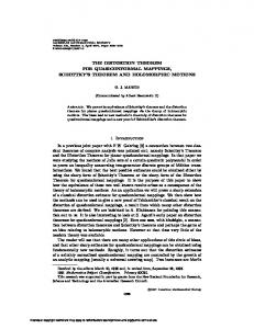
When a ≥ 1/(n−1), f satisfies the Lusin condition (N −1 ) (cf. [10]) and it follows 1,p that u◦f = uˆ ◦f almost everywhere and consequently that also u◦f ∈ Wloc (Ω1 ). ¤ 5. Construction of examples The following general construction of examples of mappings of finite distortion was introduced in [8] (see also [7]). Here we give only the brief overview of the construction, for details see [8, Section 5]. 5.1. Canonical transformation. If c ∈ Rn , a, b > 0, we use the notation Q(c, a, b) := [c1 − a, c1 + a] × · · · × [cn−1 − a, cn−1 + a] × [cn − b, cn + b] for the interval with center at c and halfedges a in the first n − 1 coordinates and b in the last coordinate. If Q = Q(c, a, b), the affine mapping ϕQ (y) = (c1 + ay1 , . . . , cn−1 + ayn−1 , cn + byn ) is called the canonical parametrization of the interval Q. Let P , P 0 be concentric intervals, P = Q(c, a, b), P 0 = Q(c, a0 , b0 ), where 0 < a < a0 and 0 < b < b0 . We set ϕP,P 0 (t, y) = (1 − t)ϕP (y) + tϕP 0 (y),

t ∈ [0, 1], y ∈ ∂Q0 .

This mapping is called the canonical parametrization of the rectangular annulus P 0 \ P ◦ , where P ◦ is the interior of P. Now, we consider two rectangular annuli, P 0 \ P ◦ , and P˜ 0 \ P˜ ◦ , where P = Q(c, a, b), P 0 = Q(c, a0 , b0 ), P˜ = Q(˜ c, a ˜, ˜b) and P˜ 0 = Q(˜ c, a ˜0 , ˜b0 ), The mapping h = ϕP˜ ,P˜ 0 ◦ (ϕP,P 0 )−1 is called the canonical transformation of P 0 \ P ◦ onto P˜ 0 \ P˜ ◦ . @ B ¡P0 @ ¡

A P A ¡ @ ¡ B @

h-

@ @ ¡ ¡

P˜

¡ ˜0 ¡ P @ @

Figure 1. The canonical transformation of P 0 \ P ◦ onto P˜ 0 \ P˜ ◦ for n = 2.

72

Stanislav Hencl and Pekka Koskela

We will need an estimate of the derivate of h on P 0 \ P ◦ . For t ∈ [0, 1] fixed we denote a00 = (1 − t)a + ta0 , b00 = (1 − t)b + tb0 , a ˜00 = (1 − t)˜ a + t˜ a0 , ˜b00 = (1 − t)˜b + t˜b0 . It is possible to compute the derivative of ϕP,P 0 (t, y) in one of the sides {yi = ±1}. The image of the side has the shape of a pyramidal frustum. We must distinguish two cases, according to the position of the first variable. Case A. We will represent the possibilities ϕP,P 0 (t, 1, z2 , . . . , zn ), ϕP,P 0 (t, −1, z2 , . . . , zn ), ... ϕP,P 0 (t, z1 , . . . zn−2 , 1, zn ), ϕP,P 0 (t, z1 , . . . zn−2 , −1, zn ) by ϕ(t, z) = ϕP,P 0 (t, 1, z),

z = (z2 , . . . , zn ).

Then it can be computed (see [8, Section 5] for details) that  a ˜0 −˜ a 0, 0, . . . , 0 −a , a ¡ ¢ 0  a ˜ −˜ a a ˜00 a ˜00 , 0, . . . ,  ¡ a0 −a − a00 ¢z2 , a00 00  a ˜00 a ˜0 −˜ a (5.1) Dh(ϕ(t, z)) =  0, aa˜00 , . . . , 0 −a − a00 z3 , a  ...  ¡ ˜b0 −˜b ˜b00 b0 −b ¢ − b00 a0 −a zn , 0, 0, . . . , a0 −a

 0 0   0.  

˜b00 b00

Case B. A representative is ³ ´ ϕ(t, z) = (ϕP,P 0 )n (t, z, 1), (ϕP,P 0 )1 (t, z, 1), . . . , (ϕP,P 0 )n−1 (t, z, 1) , z = (z1 , . . . , zn−1 ). The purpose of the permutation of coordinates is that this leads to a triangular matrix which is easier to handle. Then   ˜b0 −˜b , 0, 0, . . . , 0 0 ¢ 00 00 0  ¡ a˜0 −˜a b a˜−b  z1 , aa˜00 , 0, . . . , 0   ¡ b0 −b − a00 ab0 −a −b  a˜0 −˜a a˜00 a0 −a ¢  00 (5.2) Dh(ϕ(t, z)) =  b0 −b − a00 b0 −b z2 , 0, aa˜00 , . . . , 0  .     ¡ a˜0 −˜a a˜.00 . a. 0 −a ¢ a ˜00 − a00 b0 −b zn−1 , 0, 0, . . . , a00 b0 −b 5.2. Construction of a mapping. By V we denote the set of 2n vertices of the cube [−1, 1]n =: Q0 . The sets Vk = V × . . . × V, k ∈ N, will serve as the sets of indices for our construction. If w ∈ Vk and v ∈ V, then the concatenation of w and v is denoted by w∧ v. The following two results are proven in [8].

Mappings of finite distortion: composition operator

73

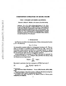
Lemma 5.1. Let n ≥ 2. Suppose that we are given two sequences of positive real numbers {ak }k∈N0 , {bk }k∈N0 , (5.3)

a0 = b0 = 1;

(5.4)

ak < ak−1 , bk < bk−1 , for k ∈ N.

Then there exist unique systems {Qv }v∈Sk∈N Vk , {Q0v }v∈Sk∈N Vk of intervals (5.5)

Qv = Q(cv , 2−k ak , 2−k bk ),

Q0v = Q(cv , 2−k ak−1 , 2−k bk−1 )

such that (5.6) (5.7)

Q0v , v ∈ Vk , are nonoverlaping for fixed k ∈ N, [ Qw = Q0w∧ v for each w ∈ Vk , k ∈ N, v∈V

(5.8) (5.9)

1 cv = v, 2 cw ∧ v = cw +

v ∈ V, n−1 X

2−k ak vi ei + 2−k bk vn en ,

i=1

w ∈ Vk , k ∈ N, v = (v1 , . . . , vn ) ∈ V.

Figure 2. Intervals Qv and Q0v for v ∈ V1 and v ∈ V2 for n = 2.

Theorem 5.2. Let n ≥ 2. Suppose that we are given four sequences of positive real numbers {ak }k∈N0 , {bk }k∈N0 , {˜ ak }k∈N0 , {˜bk }k∈N0 , (5.10) a0 = b0 = a ˜0 = ˜b0 = 1; (5.11)

ak < ak−1 , bk < bk−1 , a ˜k < a ˜k−1 , ˜bk < ˜bk−1 , for k ∈ N.

Let the systems {Qv }v∈Sk∈N Vk , {Q0v }v∈Sk∈N Vk of intervals be as in Lemma 5.1, and ˜ v }v∈S Vk , {Q ˜ 0v }v∈S Vk of intervals be associated with the similarly systems {Q k∈N k∈N sequences {˜ ak } and {˜bk }. Then there exists a unique sequence {f k } of bilipschitz homeomorphisms of Q0 onto itself such that ˜ v canonically, ˜ 0v \ Q (a) f k maps each Q0v \ Qv , v ∈ Vm , m = 1, . . . , k, onto Q k k ˜ (b) f maps each Qv , v ∈ V , onto Qv affinely. Moreover, (5.12)

|f k − f k+1 | . 2−k ,

|(f k )−1 − (f k+1 )−1 | . 2−k .

74

Stanislav Hencl and Pekka Koskela

The sequence f k converges uniformly to a homeomorphism f of Q0 onto Q0 . 5.3. Completion of the proofs of theorems 1.1 and 1.2. Construction for Theorem 1.1. It is a well-known fact that for every ε > 0 there 1,n+ε is a quasiconformal mapping f such that f ∈ / Wloc . Therefore we can assume that p < n. Choose δ > 0 such that n n−1 (5.13) δ < − 1 and δ(n − 1 + p + ε) < ε . p p Set

1 n−1 + δ, β = and γ = δ. p p With the help of (5.13) it is not difficult to verify that α=1−

(n − 1)α + β + p(γ − β) = (n − 1 + p)δ > 0 (n − 1)α + β + (p + ε)(γ − β) = (n − 1 + p + ε)δ − ε

(5.14)

(n − 1)α + β + Use Theorem 5.2 for 1 ak = , (k + 1)α

n−1 0. n−p n−p

bk =

1 , (k + 1)β

a ˜k =

1 (k + 1)γ

and ˜bk =

1 (k + 1)γ

to obtain the sequence {f k } and a limit mapping mapping f . For fixed t ∈ [0, 1] we denote a00k = (1 − t)ak + tak−1 , a ˜00k = (1 − t)˜ ak + t˜ ak−1 , Since

1 kω

−

1 (k+1)ω

∼

1 kω+1

b00k = (1 − t)bk + tbk−1 , ˜b00 = (1 − t)˜bk + t˜bk−1 . k

for every ω > 0, it is easy to check that

a ˜k−1 − a ˜k a ˜00k ∼ 00 ∼ k α−γ , ak−1 − ak ak ˜b00 ˜bk−1 − ˜bk ∼ k00 ∼ k α−γ , ak−1 − ak ak b00k bk−1 − bk ∼ 00 ∼ k α−β . ak−1 − ak ak

˜bk−1 − ˜bk bk−1 − bk

˜b00 ∼ k00 ∼ k β−γ , bk

a ˜00 a ˜k−1 − a ˜k ∼ 00k ∼ k β−γ , bk−1 − bk bk

From (5.13) we obtain that α < β and therefore it is not difficult to deduce from (5.1) and (5.2) that |Df k (x)| = |Df (x)| ∼ k β−γ (5.15)

K(x) =

and

k n(β−γ) |Df (x)|n ∼ (n−1)(α−γ)+(β−γ) = k (n−1)(β−α) Jf (x) k

Mappings of finite distortion: composition operator

75

˜ 0v \ Q ˜ v , v ∈ Vk . It is also not difficult to find out from the for almost every x ∈ Q construction that 1 ˜0 \ Q ˜v) ∼ (5.16) Ln (Q for every v ∈ Vk . v kn (n−1)α+β+1 2 k Let k < m. From (5.15), (5.16) and (5.14) we obtain Z Z ¡ ¢ k m p |Df − Df | dx . |Df k |p + |Df m |p dx Q0

. .

XZ v∈Vk m X

k p

{f k 6=f m } m X

|Df | dx + Qv

2kn

j=k

¡

j

¢ β−γ p

XZ

j=k+1 v∈Vj

2kn j (n−1)α+β+1

p

|Df | dx + Q0v \Qv

X Z v∈Vm

|Df m |p dx Qv

. k −(n−1+p)δ → 0.

It follows that the sequence {f k } converges to f in W 1,p (Q0 , Rn ) and, in particular, f ∈ W 1,p (Q0 , Rn ). From (5.14) and (5.15) we also have Z X k (p+ε)(β−γ) = ∞ and |Df |p+ε ∼ k 1+(n−1)α+β Q0 k∈N ¡ ¢ p Z X k (n−1)(β−α) n−p p < ∞. K n−p ∼ 1+(n−1)α+β k Q0 k∈N 1,p+ε By considering the functions ui (x) = xi , we see that Tf (W 1,n (Q0 )) 6⊂ Wloc (Q0 ). ¤

Construction for Theorem 1.2. Since s(q − p) − p(q − n) > 0 (i.e. a > 0) we can clearly find η > 0 small enough such that 1 η < qs + np − qp − (qp + nsp − np − qs) and n ¢− 1 (5.17) ¡ (n − 1)η + ε −ns + η + ηp < 0. Set

1 (qp + nsp − np − qs) + η, β = qs + np − qp, n−1 γ = q(s − p) + η and δ = (q − n)(s − p) + η.

α=

1 It is easy to check that β, γ and δ are positive. From a ≥ n−1 we obtain that also α is positive and (5.17) implies β > α. With the help of the definition of a and (5.17) it is not difficult to verify that

(n − 1)α + β + s(γ − β) = (n − 1)η + sη > 0 (5.18)

(n − 1)α + β + a(n − 1)(α − β) = (n − 1)η + a(n − 1)η > 0 nγ + q(δ − γ) = nη > 0

¡ ¢ (n − 1)α + β + (p + ε)(δ − β) = (n − 1)η + ε −ns + η + ηp < 0.

76

Stanislav Hencl and Pekka Koskela

Use Theorem 5.2 for the sequences 1 1 1 , bk = , a ˜k = ak = α β (k + 1) (k + 1) (k + 1)γ

and ˜bk =

1 (k + 1)γ

to obtain the sequence {f k } and a limit mapping mapping f . Analogously to the proof of the second part of Theorem 1.1 we obtain that f ∈ W 1,s and thanks to β > α and (5.18) we have Z X k s(β−γ) |Df |s ∼ < ∞ and 1+(n−1)α+β k Q0 k∈N ¡ ¢ Z X k n(β−γ)−(n−1)(α−γ)−(β−γ) a a K ∼ < ∞. 1+(n−1)α+β k Q0 k∈N Analogously, we can use Theorem 5.2 for the sequences 1 1 1 1 ˜˜b = ˜bk = ˜˜k = a ˜k = , , a and k (k + 1)γ (k + 1)γ (k + 1)δ (k + 1)δ to obtain a limit mapping g such that Z X k q(γ−δ) < ∞. |Dg|q ∼ 1+nγ k Q0 k∈N From [8, Remark 5.6] we know that the mapping h = g ◦ f can be obtained as a limit mapping from Theorem 5.2 applied to the sequences 1 1 1 1 ˜˜k = ak = , bk = , a and ˜˜bk = . α β δ (k + 1) (k + 1) (k + 1) (k + 1)δ Therefore (5.18) yields Z |Dh|p+ε ∼ Q0

X k (p+ε)(β−δ) = ∞. 1+(n−1)α+β k k∈N

To obtain a real-valued function u as indicated in the second part of Theorem 1.2, simply consider the coordinate functions of g. ¤ 6. Integrability of the distortion of f2 ◦ f1 In this section we give conditions which quarantee nice integrability of the distortion of f2 ◦ f1 . The following example shows that even if f1 and f2 and their distortions are very nice it does not follow that the distortion of their composition is nice. Example 6.1. Let n ≥ 2 and p ≥ 1. There exist homeomorphisms f1 , f2 : B(0, 1) → B(0, 1) of finite distortion such that f1 and f2 are Lipschitz, exp(K1p ) ∈ L1 (B(0, 1)) and K2 ∈ Lp (B(0, 1)), but K ∈ / Lδloc (B(0, 1)) for any δ > 0, where K denotes the distortion of the mapping f = f2 ◦ f1 .

Mappings of finite distortion: composition operator

77

Proof. Set

³ 1 x e ´ 1+ 2(n−1)p f1 (x) = e exp − log for x ∈ B(0, 1) \ {0}, kxk kxk ¡ 1¢ x f2 (x) = e exp −kxk− p for x ∈ B(0, 1) \ {0} kxk

and f1 (0) = f2 (0) = 0. From Lemma 2.1 we easily obtain that f2 is Lipschitz and that Z Z 1 p K2 (x) dx ∼ dx < ∞. n−1 B(0,1) B(0,1) kxk Analogously we obtain that f1 is Lipschitz and Z Z ³ e ´ p dx < ∞. exp(K1 (x)) dx ∼ exp C log1/2 kxk B(0,1) B(0,1) Since for every x 6= 0 we have ³ ¡1 1 e ¢´ x f (x) = e exp −e−1/p exp log1+ 2(n−1)p kxk p kxk one can use Lemma 2.1 to obtain that ¡n − 1 1 1 e ¢ e log1+ 2(n−1)p log 2p K(x) ∼ exp p kxk kxk and it is easy to check that K δ is not integrable for any δ > 0.

¤

Lemma 6.2. Let n ≥ 2, p > n − 1 and let Ω ⊂ Rn be a domain. Suppose that 1,1 f ∈ Wloc (Ω, Rn ) is a homeomorphism of finite distortion such that |Df | ∈ Ln−1,1 (Ω) loc p−n+1 p −1 1 −1 n p (e + |Df |) ∈ Lloc (f (Ω)). and K ∈ Lloc (Ω). Then |Df | log Proof. Fix a compact set E ⊂ Ω. The fact that, under our assumptions, we 1,n have f −1 ∈ Wloc (f (Ω), Rn ) and moreover that f is mapping of finite distortion follows from [8, Theorem 1.2 and Theorem 4.1]. Therefore, analogously to [8, Proof of Theorem 4.1], we obtain Z p−n+1 |Df −1 (y)|n log p (e + |Df −1 (y)|) dy f (E) (6.1) Z p−n+1 ¡ K(x) ¢ ≤ K(x)n−1 log p e + dx. |Df (x)| E Set S = {x ∈ E :

K(x) |Df (x)|

≤ exp(K p (x))}. For every x ∈ E \ S we have ¡ K p (x) ≤ C(p) log e +

¢ 1 |Df (x)|

and therefore we can split the integral in (6.1) into two parts and prove that it is no greater than Z Z ¡ ¢ ¡ ¢ 1 n−1 p−n+1 K(x) C(p) + K (x) dx + C(p) log e + dx. |Df (x)| E E

78

Stanislav Hencl and Pekka Koskela

The finiteness of the first integral follows from K ∈ Lp (E). Analogously to [7, Theorem 6.1], one can prove that log(1 + |J1f | ) ∈ L1loc (Ω) for every n ≥ 2, which implies that the second integral is also finite. ¤ It follows from the Example 6.1 that if we want to prove the integrability of some power of the distortion of f2 ◦ f1 , we must require some stronger condition than the integrability of some power of the distortion of f2 . Theorem 6.3. Let n ≥ 2, Ω ⊂ Rn be a domain, p > n − 1 and r > 0 and set pr(p−n+1) 1,1 1,n q = r(p−n+1)+p(p+1) . Suppose that f1 ∈ Wloc (Ω, Rn ) and f2 ∈ Wloc (f1 (Ω), Rn ) are homeomorphisms with finite distortion such that |Df1 | ∈ Ln−1,1 (Ω), K1 ∈ Lp (Ω) ¡ r¢ and exp 2K2 ∈ L1loc (f1 (Ω)). Then f = f2 ◦ f1 is a mapping of finite distortion and its distortion satisfies K ∈ Lqloc (Ω). 1,1 Proof. From Theorem 1.1 we know that f ∈ Wloc (Ω, Rn ). We claim that for almost every x ∈ Ω we have

(6.2)

Df (x) = Df2 (f1 (x))Df1 (x) and Jf (x) = Jf2 (f1 (x))Jf1 (x).

From [3] we know that we can find a Borel partition of f1 (Ω), {Ak }, such that |A0 | = 0 and f2 is Lipschitz on Ak , k > 0. We know that f1 is differentiable almost everywhere (see [14]) and that f2 restricted to Ak is differentiable almost everywhere. Since f1 satisfies the Lusin (N −1 ) condition (see [10, Theorem 1.2]) it is not difficult to deduce that (6.2) holds almost everywhere on f1−1 (Ak ) for every k > 0. The Lusin (N −1 ) condition also gives us |f1−1 (A0 )| = 0 and therefore (6.2) holds almost everywhere. Since f1 and f2 are mappings of finite distortion and f2 satisfies the Lusin (N −1 ) condition, we can deduce from (6.2) that f is also a mapping of finite distortion. Let A ⊂⊂ Ω be a fixed Borel set such that f1 is differentiable at A (recall that this happens almost everywhere in Ω [14]) and that |Df (x)| > 0 for every x ∈ A. Set (6.3)

s=

p2 r(p − n + 1) + p(p + 1)

and check that clearly 0 < s < 1. The definition of distortion, (6.2) and the Hölder’s inequality give us Z

Z

q

|Df2 (f1 (x))|nq Jf1 (x)s |Df1 (x)|n(q+s) dx Jf2 (f1 (x))q |Df1 (x)|ns Jf1 (x)q+s A ³Z ´s ³Z ´1−s q+s q Jf1 (x) 1−s s ≤ K2 (f1 (x)) dx K (x) dx . 1 |Df1 (x)|n A A

K (x) dx ≤ A

q+s Clearly 1−s = p, which implies that the second integral is finite and therefore it is enough to prove the finiteness of the first integral. By (2.1), Df1 (f1−1 (y))Df1−1 (y) =

Mappings of finite distortion: composition operator

79

I and (2.2) for α = p−n+1 we have p Z Z q q Jf1 (x) −1 n s s K2 (f1 (x)) dx ≤ K 2 (y)|Df1 (y)| dy n |Df (x)| 1 A f1 (A) Z qp ¢ ¡ s(p−n+1) ≤ C (y) exp 2K2 (6.4) f1 (A) Z p−n+1 +C |Df1−1 (y)|n log p (e + |Df1−1 (y)|) dy. f1 (A)

The boundedness of the first integral follows from (6.3) and our assumptions and the boundedness of the second follows from Lemma 6.2. ¤ References [1] Astala, K., T. Iwaniec, P. Koskela, and G. Martin: Mappings of BMO-bounded distortion. - Math. Ann. 317, 2000, 703–726. [2] David, G.: Solutions de l’equation de Beltrami avec kµk∞ = 1. - Ann. Acad. Sci. Fenn. Ser. A I Math. 13:1, 1988, 25–70. [3] Federer, H.: Geometric measure theory. - Die Grundlehren der mathematischen Wissenschaften, Band 153, Springer-Verlag, New York, 1969 (second edition 1996). [4] Gehring, F. W., and J. Väisälä: Hausdorff dimension and quasiconformal mappings. - J. London Math. Soc. 6, 1973, 504–512. [5] Gutlyanski˘ı, V., O. Martio, T. Sugawa, and M. Vuorinen: On the degenerate Beltrami equation. - Trans. Amer. Math. Soc. 133:5, 2005, 1451–1458. [6] Hedberg, L. I.: On certain convolution inequalities. - Proc. Amer. Math. Soc. 36, 1972, 505–512. [7] Hencl, S., and P. Koskela: Regularity of the inverse of a planar Sobolev homeomorphism. - Arch. Ration. Mech. Anal. 180, 2006, 75–95. [8] Hencl, S., P. Koskela, and J. Malý: Regularity of the inverse of a Sobolev homeomorphism in space. - Proc. Roy. Soc. Edinburgh Sect. A 136:6, 2006, 1267–1285. [9] Kauhanen, J., P. Koskela, and J. Malý: Mappings of finite distortion: condition N. Michigan Math. J. 49, 2001, 169–181. [10] Koskela, P., and J. Malý: Mappings of finite distortion: the zero set of the Jacobian. - J. Eur. Math. Soc. 5:2, 2003, 95–105. [11] Lehto, O., and K. I. Virtanen: Quasiconformal mappings in the plane. - Springer-Verlag, 1973. [12] Malý, J., P. Swanson, and W. P. Ziemer: The co-area formula for Sobolev mappings. Trans. Amer. Math. Soc. 355:2, 2002, 477–492. [13] Martio, O., V. Ryazanov, U. Srebro, and E. Yakubov: On Q-homeomorphisms. - Ann. Acad. Sci. Fenn. Math. 30:1, 2005, 49–69. [14] Onninen, J.: Differentiability of monotone Sobolev functions. - Real Anal. Exchange 26:2, 2000, 761–772.

80

Stanislav Hencl and Pekka Koskela

[15] Rickman, S.: Quasiregular mappings. - Ergeb. Math. Grenzgeb. (3) 26, Springer-Verlag, Berlin, 1993. [16] Ryazanov, V., U. Srebro, and E. Yakubov: BMO-quasiconformal mappings. - J. Anal. Math. 83, 2001, 1–20. [17] Stein, E. M., and G. Weiss: Introduction to Fourier analysis on Euclidean spaces. - Princeton Univ. Press, 1971. [18] Ukhlov, A. D.: On mappings generating the embeddings of Sobolev spaces. - Siberian Math. J. 34:1, 1993, 165–171. [19] Väisälä, J.: Lectures on n-dimensional quasiconformal mappings. - Springer, 1971. [20] Ziemer, W. P.: Change of variables for absolutely continuous functions. - Duke Math. J. 36:1, 1969, 171–178. [21] Ziemer, W. P.: Weakly differentiable functions. - Grad. Texts in Math. 120, Springer-Verlag, 1989.

Received 24 February 2006