Aug 27, 2012 - comply with user-defined business rules and requirements. Cur- ..... Hive and Pig and show that ETLMR-based code is shorter and very.
MapReduce-based Dimensional ETL Made Easy Xiufeng Liu, Christian Thomsen, Torben Bach Pedersen Dept. of Computer Science, Aalborg University, Denmark {xiliu, chr, tbp}@cs.aau.dk
ABSTRACT
SCDs, etc. This results in low ETL programmer productivity. To implement a parallel dimensional ETL program on MapReduce is thus still very costly and time-consuming due to the inherent complexities of ETL-specific activities when processing dimensional DW schemas with SCDs etc. In this demonstration, we present the MapReduce-based framework ETLMR [2] (the code is freely available from etlmr.cs. aau.dk). ETLMR offers high-level ETL-specific constructs on fact tables and dimensions (including SCDs) in both star schemas and snowflake schemas. A user can implement parallel ETL programs by using these constructs without knowing the details of the parallel execution of the ETL processes. This makes MapReducebased ETL very easy. It reduces tedious programming work such that the user only has to make a configuration file with few lines of code to declare dimension and fact objects and the necessary transformation functions. ETLMR achieves this by using and extending pygrametl [4], a Python-based framework for easy ETL programming. Figure 1 shows parallel ETL using ETLMR. The ETL flow consists of two sequential phases: dimension processing and fact processing. Data is read from the sources, i.e., files on a distributed file system (DFS), transformed, and processed into dimension values and facts by parallel ETLMR instances which consolidate the data in the DW. To make a parallel ETL program, only few lines of code declaring target tables and transformation functions are needed.
This paper demonstrates ETLMR, a novel dimensional Extract– Transform–Load (ETL) programming framework that uses MapReduce to achieve scalability. ETLMR has built-in native support of data warehouse (DW) specific constructs such as star schemas, snowflake schemas, and slowly changing dimensions (SCDs). This makes it possible to build MapReduce-based dimensional ETL flows very easily. The ETL process can be configured with only few lines of code. We will demonstrate the concrete steps in using ETLMR to load data into a (partly snowflaked) DW schema. This includes configuration of data sources and targets, dimension processing schemes, fact processing, and deployment. In addition, we also present the scalability on large data sets.
1. INTRODUCTION In data warehousing, ETL flows are responsible for collecting data from different data sources, transformation, and cleansing to comply with user-defined business rules and requirements. Current ETL technologies are demanded to process many gigabytes of data each day. The vast amount of data makes ETL extremely time-consuming. The use of parallelization technologies is the key to achieve better ETL scalability and performance. In recent years, the “cloud computing” technology MapReduce [1] has been widely used for parallel computing in data-intensive areas due to its good scalability. We see that MapReduce can be a good foundation for ETL parallelization. ETL processing exhibits the composable property such that the processing of dimensions or facts can be split into smaller computations and the partial results from these computations can be merged to constitute the final results in a DW. Further, the MapReduce programming paradigm is very powerful and flexible. MapReduce makes it easier to write a distributed computing program by providing interprocess communication, fault-tolerance, load balancing, and task scheduling. It is often said that while parallel DBMSs are good for querying of large data sets, MapReducebased systems are good for ETL tasks and that a MapReduce-based ETL system thus can live upstream from the DBMS [3]. However, MapReduce is a general framework and lacks support for highlevel ETL-specific constructs such as star and snowflake schemas,
Figure 1: Parallel ETL using ETLMR In the demonstration, we will focus on a complete scenario where we process data for a partly snowflaked schema which also has an SCD. We demonstrate the configuration of data sources and targets, three dimension processing schemes, and fact processing as well as deployment and scalability. For a full description of the research challenges in making ETLMR, we refer to [2].
Permission to make digital or hard copies of all or part of this work for personal or classroom use is granted without fee provided that copies are not made or distributed for profit or commercial advantage and that copies bear this notice and the full citation on the first page. To copy otherwise, to republish, to post on servers or to redistribute to lists, requires prior specific permission and/or a fee. Articles from this volume were invited to present their results at The 38th International Conference on Very Large Data Bases, August 27th - 31st 2012, Istanbul, Turkey. Proceedings of the VLDB Endowment, Vol. 5, No. 12 Copyright 2012 VLDB Endowment 2150-8097/12/08... $ 10.00.
2. SOURCES AND TARGETS Throughout the demonstration, we use a running example inspired by a project which tests web pages with respect to accessibility (i.e., the usability for disabled people) and conformance to certain standards. Each test is applied to all pages. For each
1882
(sometimes referred to as the “business key”). Besides, optional parameters can be given, such as a default value for the dimension key when a dimension value is not found in a lookup, e.g., defaultid=-1 in the declaration of testdim. For an instance of SlowlyChangingDimension, additional SCD related parameters – such as the columns for the version number and the timestamps – are given. Note how easy it is to declare and use a snowflaked SCD in ETLMR. This is very complex with traditional tools. Other settings of the dimension tables for different processing schemes are discussed later.
page, the test outputs the number of errors detected, and the results are written to a number of tab-separated files which form the data sources. The data is split into approximately equal-sized files and uploaded to the DFS (this is also where the results of previous MapReduce jobs are written if other MapReduce jobs must process the data before ETLMR). The files are located by URLs. # Define the sources in the main program paralleletl.py: fileurls = [’dfs://localhost/TestResults0.csv’, ’dfs://localhost/TestResults1.csv’, ...]
Lines from the input files are read into Python dictionaries for manipulation in ETLMR. Here, we call them rows and they map attribute names to values. An example of a row is
3. DIMENSION PROCESSING SCHEMES
row={’url’:’www.dom0.tl0/p0.htm’, ’size’:’15998’, ’serverversion’:’MyServer/1.0’, ’downloaddate’ :’2011-01-31’,’lastmoddate’:’2011-01-01’, ’test’ :’Test001’, ’errors’:’7’}
ETLMR has several dimension processing schemes. We will demonstrate how to configure and choose the schemes.
3.1
Figure 2 shows the partly snowflaked target schema (ETLMR supports star and snowflake schemas, and their combinations). The schema comprises testdim, datedim, five snowflaked page dimension tables, and the fact table testresultsfact. pagedim is an SCD. The declarations of the dimension tables are seen in the following (we show the declaration of the fact table in Section 4).
One Dimension One Task
We first consider an intuitive approach to process dimensions in parallel, namely “one dimension, one task” (ODOT) where there is one (and only one) map/reduce task for each dimension table. We first define the corresponding attributes of the data source for each dimension table (the srcfields) and transformations (the rowhandlers). The user implements transformations as normal Python functions and can thus do advanced cleansing and transformations. The transformations are applied to each processed row. For space reasons, we do not show definitions of our transformations but only refer to their self-explanatory names (“UDF ...”).
Figure 2: The running example # Declared in the configuration file, config.py from odottables import * # Declare the dimensions: testdim=CachedDimension(name=’test’,key=’testid’,defaultid\ =-1,attributes=[’testname’], lookupatts=[’testname’]) datedim = CachedDimension(name=’date’,key=’dateid’, attributes=[’date’,’day’,’month’, ’year’,’week’], lookupatts=[’date’]) # Declare the dimension tables of the normalized pagedim. pagedim = SlowlyChangingDimension(name=’page’, key=’pageid’, lookupatts=[’url’], attributes=[’url’, ’size’,’validfrom’,’validto’,’version’,’domainid’, ’serverversionid’], versionatt=’version’, srcdateatt=’lastmoddate’, fromatt=’validfrom’, toatt=’validto’) topdomaindim=CachedDimension(name=’topdomaindim’, key=’topdomainid’,attributes=[’topdomain’], lookupatts=[’topdomain’]) domaindim = CachedDimension(name=’domaindim’, key=’domainid’,attributes=[’domain’,’topdomainid’], lookupatts=[’domain’]) serverdim = CachedDimension(name=’serverdim’,key=\ ’serverid’,attributes=[’server’], lookupatts=[’server’]) serverversiondim=CachedDimension(name=’serverversiondim’, key=’serverversionid’,attributes=[’serverversion’, ’serverid’], lookupatts=[’serverversion’], refdims=[serverdim]) # Define the references in the snowflaked dimension: pagesf=SnowflakedDimension( (pagedim, (serverversiondim, domaindim)), (serverversiondim,serverdim),(domaindim, topdomaindim))
Different parameters are given when declaring a dimension table instance (here we use CachedDimension instances which cache parts of the data in memory), including the dimension table name, the key column, and lists of attributes and lookup attributes
1883
# Defined in config.py dims={ pagedim:{’srcfields’:(’url’,’serverversion’,’domain’, ’size’, ’lastmoddate’), ’rowhandlers’:(UDF_extractdomain,UDF_extractserverver)}, domaindim:{’srcfields’:(’url’,), ’rowhandlers’:(UDF_extractdomain,)}, topdomaindim:{’srcfields’:(’uri’,), ’rowhandlers’:(UDF_extracttopdomain,)}, serverversiondim:{’srcfields’:(’serverversion’,), ’rowhandlers’:(UDF_extractserverver,)}, serverdim:{’srcfields’:(’serverversion’,), ’rowhandlers’:(UDF_extractserver,)}, datedim:{’srcfields’:(’downloaddate’,), ’rowhandlers’:(UDF_explodedate,)}, testdim:{’srcfields’:(’test’,), ’rowhandlers’:()} }
As there are references between the tables of the snowflaked (normalized) dimension, the processing order matters and is specified in the following. It is illustrated in Figure 3. order=[(’topdomaindim’, ’serverdim’), (’domaindim’, ’serverversiondim’), (’pagedim’, ’datedim’, ’testdim’)]
Figure 3: Process snowflake schema With this order, the dimensions are processed from the leaves towards the root (the dimension table referenced by the fact table is the root and a dimension table without a foreign key to another dimension tables is a leaf). The dimension tables with dependencies (from foreign key references) are processed in sequential jobs, e.g., Job1 depends on Job0, and Job2 depends on Job1. Each job processes independent dimension tables by parallel tasks. Therefore, Job0 first processes topdomaindim and serverdim, then
Job1 processes domaindim and serverversiondim, and finally Job2 processes pagedim, datedim, and testdim. When processing, ETLMR does data projection in the mappers to select the necessary values for each dimension table. This results in key/value pairs of the form (dimension table name, tuple of values) that are given to the reducers. ETLMR partitions the map outputs based on the table names such that the values for one dimension table are processed by a single reducer (see Figure 4). For example, the reducer for pagedim receives among others the values {’url’:’www.dom0.tl0/p0.htm’,’serverversion’: ’Xyz/1.0’,’size’:’12’,’lastmoddate’:’2011-01-01’}. In the reducers, ETLMR automatically applies UDFs for transformations (if any) to each row. The row is then automatically ensured to be in the dimension table, i.e., ETLMR inserts the dimension value if it does not already exist in the dimension table, and otherwise updates it as needed. For a type-2 SCD (where versioning of rows is applied), ETLMR also adds a new version and updates the valid timestamps of the old version as needed. The programmer thus only has to program the transformations to apply and ETLMR takes care of the rest.
Figure 4: ODOT
3.2
Figure 6: Before post-fixing
Figure 7: After post-fixing
table and improper values in the SCD attributes, validfrom, validto, and version. The post-fixing program first fixes the topdomaindim such that rows with the same value for the lookup attribute are merged into one row with a single ID. Thus, the two rows with topdom = tl2 are merged into one row. The references to topdomaindim from domaindim are also updated to reference the correct (fixed) rows. In the same way, pagedim is updated to merge the two rows representing www.dom2.tl2. Finally, pagedim is updated. Here, the post-fixing also has to fix the values for the SCD attributes.
Figure 5: ODAT
One Dimension All Tasks
3.3
We now consider another approach to process dimensions (see Figure 5), namely “One dimension, all tasks” (ODAT). This approach makes use of all the reducers to process the map outputs, i.e., one dimension is processed by all tasks unlike ODOT where only a single task is utilized for a dimension. Thus ODAT can use more nodes and has better scalability. ETLMR has a separate Python module implementing this approach, and only a single line, from odattables import *, is needed to use it. As the ODAT dimension and fact classes have the same interfaces as the ODOT classes, nothing is changed in the declarations in Section 2, except that the processing order is not needed any more. With ODAT, the map output is partitioned in a round-robin fashion such that all reducers receive an almost equal-sized map output containing key/values pairs for all dimension tables (see Figure 5). A reducer processes map output for all dimension tables. Therefore, a number of issues need to be considered, including the uniqueness of dimension keys, concurrency problems when different tasks are operating on the same dimension values to update the timestamps of SCD dimensions, and duplicated values of the same dimension. To remedy this, ETLMR automatically employs an extra step called post-fixing to fix the problematic data when the dimension processing job has finished. Figures 6 and 7 illustrate post-fixing. The details about the post-fixing steps can be found in [2]. An embedded DBMS is used for “bookkeeping” for postfixing. This DBMS can maximally handle ∼140 terabytes of data. Post-fixing Consider two map/reduce tasks, task 1 and task 2, which process the snowflaked dimension page. Each task uses a private ID generator. The root dimension, pagedim, is a type-2 SCD. Both task 1 and task 2 process rows with the lookup attribute value url=’www.dom2.tl2/p0.htm’. Figure 6 depicts the resulting data in the dimension tables. White rows were processed by task 1 and grey rows were processed by task 2. Each row is labelled with the taskid of the task that processed it. The problems include duplicated IDs in each dimension
Offline Dimensions
ETLMR also has a module for processing dimensions which are stored on the nodes. We say such dimensions are offline as opposed to the previously described approaches where the dimensions reside in the DW database and are online. The interface of offline dimensions is similar to that of online dimensions except that there is an additional parameter, shelvedpath, to denote the local path for saving the dimension data. The following code snippet exemplifies a declaration: from offdimtables import * datedim = CachedDimension( name=’date’, key=’dateid’, attributes=[’date’,’day’,’month’,’year’,’week’], lookupatts=[’date’], shelvedpath=’/path/to/datedim’ )
When offline dimensions are used, the map/reduce tasks do not interact with the DW by means of database connections and as the data is stored locally in each node, the network communication cost is greatly reduced. The dimension data is expected to reside in the nodes, and is not loaded into the DW until this is explicitly requested.
3.4
How to Choose
The ODOT scheme is preferable for small-sized dimensions when high scalability is not required. On the contrary, the ODAT scheme is preferable for dimension tables with big data volumes as the data can processed by all tasks which gives better scalability. When immediate data availability is not required, the offline dimension scheme can be chosen for better performance.
4. FACT PROCESSING We now demonstrate how to configure the fact processing. For our example, the fact table is declared as below:
1884
Table 1: The time of dimension processing
# In config.py # Declare the fact table (here we support bulk loading): testresultsfact = BulkFactTable(name=’testresultsfact’, keyrefs=[’pageid’,’testid’,’dateid’],measures=[’errors’], bulkloader=UDF_pgcopy, bulksize=5000000)
no. of tasks Time (min)
4 260.95
8 135.65
12 91.39
16 70.73
20 55.22
in processing the big dimension. The speedup is nearly linear as the partitioning costs become more dominating when each map/reduce task gets less data and run for a shorter time. Further, the costs from the MapReduce framework (e.g., for communication) increase when more tasks are added. We also consider another 80 GB data set which has small-sized dimensions (19,460 rows in the page dimension) to study the scalability. Figure 8 shows ETLMR has a nearly linear speedup in the increasing number of tasks. When we use a fixed number of tasks (such that the MapReduce costs don’t increase) and vary the size of the test data, the processing time grows linearly in the data size (see Figure 9).
Speedup, T1 /Tn
It is possible to declare several fact tables if needed, and they can be processed in parallel. The declaration of a fact table includes the name of the fact table and the column names of the dimensionreferencing keys and measures. Here, the BulkFactTable class is used to enable bulk loading of facts. As the bulk loader varies from DBMS to DBMS, the user has to declare which function to call to perform the actual bulk loading. After the declaration, ETLMR must be configured to use the instance. This involves specifying the dimension objects from which ETLMR looks up dimension keys and specifying the transformations (“rowhandlers”) which ETLMR should apply to the facts. When ETLMR processes the fact data, the data files are assigned to the map/reduce tasks in a round-robin fashion. Each task automatically does its work by applying the user-defined transformations to the rows from the data files, looking up dimension keys, and inserting the rows into a buffer. When the buffer is full, its data is loaded into the DW by means of the bulk loader. This is again very easy for the user who just has to program transformations.
24 22 20 18 16 14 12 10 8 6 4 2 0
300 Compared with 1 task
Processing time (min.)
# Set the referenced dimensions and the # transformations to apply to facts: facts = {testresultsfact: {’refdims’:(pagedim, datedim, testdim), ’rowhandlers’:(UDF_convertStrToInt,)}}
0
5. DEPLOYMENT
4 tasks 8 tasks 12 tasks
16 tasks 20 tasks
200 150 100 50 0 20
4 8 12 16 20 The number of tasks, n
Figure 8: Speedup with increasing tasks, 80GB
250
40 60 Data size (GB)
80
Figure 9: Processing time when scaling up data size
More studies of the scalability can be found in [2] which also considers the use of ETLMR compared to doing ETL operations by means of the MapReduce tools Hive and Pig. As ETLMR is a specialized ETL tool, it is much simpler to create an ETL solution with ETLMR. Further, [2] compares the performance of ETLMR to the leading open source ETL tool PDI which also supports MapReduce. In the comparison, ETLMR is significantly faster.
ETLMR uses the Python-based Disco (discoproject.org) as its MapReduce platform. The system uses a master/worker architecture with one master and many workers (or nodes). Each worker has a number of map/reduce tasks which run the ETLMR parts in parallel. The master is responsible for scheduling the tasks, distributing partitioned data, tracking status, and monitoring the status of workers. If a worker crashes, the MapReduce framework automatically assigns the node’s task to another node and thus provides us with restart and checkpointing capabilities. To deploy ETLMR, a configuration module is placed on the master. This configuration defines dimension and fact tables. The distributed ETL program is then started by the following code which defines which node is the master, where the input is located, the name of the configuation module, and the numbers of mappers and reducers.
7. DEMONSTRATION
# Start the ETLMR main program, paralleletl.py: ETLMR.start(master=’masternode’,inputs=fileurls,required_\ modules=[(’config’,’config.py’)],nr_maps=20,nr_reduces=20)
We note that the number of mappers and reducers can easily be changed in this program by only updating the nr maps and nr reduces arguments. This makes it very easy for the ETL developer to scale up/scale down ETL programs.
In the demonstration, we will show how to implement a MapReduce-based dimensional ETL program using ETLMR. We will use the running example of this paper – a (partly) snowflaked schema with an SCD – as our demonstration case and show how to build a complete ETL program in few lines by using the constructs shown in Sections 2–5. We will thus show the configuration of data sources, targets, and transformations. Further, we will show how to choose between ETLMR’s different processing schemes, how the schemes differ, and how post-fixing works for the ODAT scheme. Finally, we will compare ETLMR to the MapReduce-based tools Hive and Pig and show that ETLMR-based code is shorter and very intuitive. The audience will thus experience the programming efficiency in creating highly parallel ETL-programs with ETLMR.
8. REFERENCES
6. SCALABILITY
[1] J. Dean and S. Ghemawat, “MapReduce: Simplified Data Processing on Large Clusters”. In Proc. of OSDI, pp. 137–150, 2004. [2] X. Liu, C. Thomsen and T. B. Pedersen, “ETLMR: A Highly Scalable ETL Framework Based on MapReduce”. In Proc. of DaWaK, pp. 96–111, 2011. [3] M. Stonebraker et al., “MapReduce and Parallel DBMSs: friends or foes?”. CACM, 53(1):64–71, 2010. [4] C. Thomsen and T. B. Pedersen, “pygrametl: A Powerful Programming Framework for Extract-Transform-Load Programmers”. In Proc. of DOLAP, pp. 49–56, 2009.
We now present the scalability of ETLMR. Details about the used cluster are available in [2]. Table 1 shows the time of dimension processing when we use the ODAT and offline dimension processing scheme (the fastest). We use an 80 GB fixed-size data set for the running example represented in a star schema (with 13,918,502 rows in the page dimension). We scale the number of map/reduce tasks from 4 to 20. As the data is equally split and processed by all tasks, ETLMR achieves a nearly linear speedup
1885