Market foreclosure and exclusivity contracts when ... - CiteSeerX

Market foreclosure and exclusivity contracts when consumers have switching costs* Tommaso M. Valletti** London School of Economics Politecnico di Torino and Centre for Economic Policy Research This version: July 1999 Comments are welcome Abstract In the presence of switching costs, firms are often interested in expanding current market shares to exploit their customer base in the future. However, if the product is sold by retailers, manufacturers may face the problem of extracting too much surplus from the retailer. If this happens, then the latter has not an incentive to build a subscriber base. This paper would like to draw a line between two unrelated streams in the literature, respectively on switching costs and vertical restraints. An upstream-downstream duopoly model is presented to analyse the mutual incentive for firms to enter into particular trading relationships when consumers are repeat-purchasers. When switching costs are high, then integrated structures are predicted (or exclusive dealership in case vertical integration is banned). On the other hand, when lock in effects are not too relevant, mixed structures with independent firms are particularly likely to emerge in growing industries (independent firms can be made of latecomers not entering in the initial stages of competition). Keywords: switching costs, vertical restraints, integration, foreclosure, exclusivity

*

This is a substantially revised version of a previous paper circulated with the title "Switching costs in vertically related markets". I am grateful to Pedro Pita Barros, David Salant, John Sutton and seminar participants at LSE, Lisbon, Madrid, Stockholm, EARIE 1997 and ESEM 1997 for useful discussions and comments. ** Address for correspondence: Department of Economics, LSE, Houghton Street, London WC2A 2AE, UK. E-mail: [email protected]

1.

Introduction

Consumer switching costs make changing suppliers expensive and tend to lock consumers into the firms they were previously patronising. If those who buy from a firm now have a desire to buy from the same firm next period, then it is natural that increasing market share is in the firm's interest. When entry is allowed, incumbents may also strategically expand output and attract consumers, making entry more difficult and exerting monopolistic power on those that are locked in. In a stylised two-period model of switching costs, a firm is usually willing to serve a larger set of customers in the first period than in traditional models because this enlarges its 'captive' segment of the market in the following period. This theory of heightened competition for market shares in the initial phase justifies strategies like giving cheap introductory offers to new customers, even if such behaviour involves some sacrifice of short-run profit. Switching costs lead to rents, but in turn these rents induce greater competition in the early stages of the market's development. Thus firms face a trade-off between future profits and present losses caused by the aggressive first-period behaviour. The net effect is often ambiguous and switching costs can actually make firms worse off (Klemperer, 1987).1 The literature on switching costs has found important implications for many questions of industrial economics (see Klemperer, 1995, for a survey of recent work). However, all models assume that the product is sold by the manufacturer himself. This is a good first approximation from a theoretical standpoint, and in many cases it is also reflected in reality. Banks - with high transaction costs in closing an account with one firm and opening another with a competitor - are a good example. In other cases, especially for many consumer purchases, it is possible to draw a clear distinction between manufacturers' brands and retailers' services associated with its characteristics or location and it becomes more questionable whether it is satisfactory to model manufacturing and retailing operations carried by the same firm. Products with high 'brand loyalty' can be sold in supermarkets, or alternatively the producer may decide to retail the good directly or using exclusive dealers. Computers and software compatible with them, are products that involve substantial 'learning' costs: What is the best strategy to sell the combined product? Cars, it is said, are also associated with strong brand loyalty ('psychological' costs) and, in virtually all cases, car manufacturers decide to sell using a single retailer in a given territory or similar forms of franchise systems. Even airlines with 'frequent-flyer' 1

Switching costs can also explain why prices can be higher with identical firms than with differentiated ones. If firms differentiate their products, some consumers may decide to switch firm despite they incur in some costs. On the other hand, if firms offer functionally identical products, then product characteristics cannot be a reason to patronise the other firm. In this sense, switching costs represent an artificial way of product differentiation rather than a real one (Klemperer, 1995).

1

programmes - perhaps the most cited example of a product involving switching costs may indeed sell their tickets using travel agents that do not necessarily coincide with the airline carrier. The main business cases that motivate this paper can be found in the telecommunications industry: network operators can sell services to the final users or recur to service providers: this is true for Internet services, value-added services, mobile telecoms, etc., all situations including consumer switching costs (additional software or hardware needed, change of number, etc.). The following table, borrowed from Shapiro and Varian (1999) shows how, at a more general level, switching costs and lock-in effects are ubiquitous in information systems. Type of lock-in Contractual commitments Durable purchase Brand-specific training

Switching costs Compensatory or liquidated damages Replacement of equipment; tends to decline as the durable ages Learning a new system, both direct cost and lost productivity; tends to rise over time Information and databases Converting data to new format; tends to rise over time as collection grows Specialized suppliers Funding of new supplier; may rise over time if capabilities are hard to find Search costs Combined buyer and seller search costs; includes learning about quality of alternatives Loyalty programs Any lost benefits from incumbent supplier, plus possible need to rebuild cumulative use Table 1: Types of lock-in and associated switching costs (source: Shapiro and Varian, 1999, p. 117) Once the distinction between manufacturers and retailers is introduced, it is not clear whether the manufacturer can easily delegate to the retailer the task of acquiring market shares. Vertical arrangements take a variety of forms, and they have been studied by a very rich literature on vertical integration, vertical restraints and market foreclosure (surveys can be found in Katz, 1989, Waterson, 1993, Irmen, 1998, and Rey and Tirole, 1999). The literature has focused on several issues, including the elimination of successive mark-ups, or the attempt to raise rivals' costs. Among the strategic motives for the existence of vertical separation, some authors have considered the case that separate firms can induce more friendly behaviour from rivals. In other situations, a supplier may appropriate a large share of the downstream industry profit via exclusivity contracts, price discrimination, or vertical integration. However, no reference is made to the fact that market power may arise from the existence of consumer switching costs. In such a case, a model of an upstream/downstream industry would have to include additional features

2

such as a time dimension and a mechanism to allocate future rents among the verticallyrelated firms. This paper would like to draw a line between these two streams in the literature by exploring the implication of switching costs on the firm's internal organisation and on its supply relationships. It is well known that the vertical integration of a downstream monopolist and an upstream monopolist is profitable, since it eliminates double marginalisation. The situation is more complicated in an oligopoly context. In this paper I consider a framework where two upstream firms can supply two downstream firms and firms compete at both stages of production, after having made their decisions about integration. At first, I consider simple but 'natural' contracts, starting with vertical integration and complete independence. I address the question of the contractual choice by considering a game in which pairs of firms decide which contract to sign based on anticipated profits that would occur in subsequent stages. This of course requires the solution of situations where integrated and non-integrated pairs coexist. The contract games that I study do not assume that integrated firms do not trade with non-integrated firms, rather I analyse if foreclosure may arise in equilibrium. I show that the presence of switching costs has a strong influence on market foreclosure. Since customers are eventually locked in with a retailer, by foreclosing a retailer, an upstream firm may renounce to part of the rent extractable from the captured customer in later stages of the game. At the same time, foreclosure in the initial phases may limit expensive battles for market shares. I will show that the incentive to invest in market share can be so high that an independent retailer is completely preempted in the initial phase of the game, while it recurs to an independent manufacturer in later stages. In the opening paragraph, I mentioned the basic trade-off faced in a given period by an integrated firm. If it invests in market share by charging a low price, it attracts customers that will be profitable repeat-purchasers; on the other hand, the firm can harvest profits by charging high prices to existing customers, but it also runs down the stock of market share. When independent retailers sell the product, new factors enter the picture. Manufacturers may face the paradoxical problem of extracting too much surplus from the retailer. If this happens, then the latter is not interested in building a subscriber base, resulting in foregone future profits. In this case, it is likely that firms would look for a suitable contractual solution. For instance, the problem could be reduced if retailers have the freedom to recur to alternative sources of input supply. This ensures a reservation payoff to the retailer related to what he could get if he supplied the competing manufacturer's product to his customers. Such a reservation payoff depends on the contract chosen by the rival pair: if the rival manufacturer has a complete exclusivity deal, then it cannot supply any other retailer. This is the second theme that

3

emerges in this paper: I study alternative exclusivity contracts to understand when partial competition from the other manufacturer can give credible incentives to a retailer to invest in market share when long-term contracts are not available. Alternatively, vertical integration is a candidate to emerge, so that the problem is completely internalised. On the other hand, if today's battle for market shares is too costly, then a retailer that does not 'invest' too much, may be good overall since it does not dissipate current profits. However, it is not clear at first sight whether independent pairs of firms are able to coordinate on the most profitable contractual choices and I provide a framework suitable for analysing the equilibrium contracts and their properties. The remainder is organised as follows. Section 2 presents a simple upstreamdownstream model to analyse the mutual incentive for firms to enter into particular trading relationships in the presence of switching costs. The model is solved in section 3, where the focus is on foreclosure and pre-emption. Section 4 amends the basic model to study the case of exclusive dealerships. Section 5 concludes and discusses an application to the mobile communications industry and possible extensions.

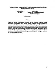
2. The model Costs and vertical structure. The market comprises two upstream manufacturers (I will also refer to them as 'network operators') indexed by h, k = A, B and two downstream retailers ('service providers'), indexed by i, j = 1, 2. In absence of switching costs, products are homogeneous and can be produced and sold by any pair once a link is established. The thin line in the figure below represents potential links, but it will be determined endogenously which potential links are established by contractual configurations. One unit of the upstream good is needed to produce one unit of the final good. Production exhibits constant return to scale. For the sake of simplicity, marginal costs are normalised to zero.

A

B

upstream manufacturers

1

2

downstream retailers

consumers

4

Demand. There are two periods of time. Downstream firms (or divisions) 1 and 2 get respectively n1 and n2 customers at t = 1 in the following manner. Firms decide how many customers to supply. When firm i connects ni customers, then the resulting price is p = a - (n1 + n2).2 At t = 2, there is consumption according to a linear demand function. Individual demand of each customer is: x = b - p. Positive parameters a and b define the relative importance of the markets in the two periods. Some customers are completely locked in after the initial purchase (they have infinite switching costs) and some of them are free to change supplier in the second period. Let 0 ≤ µ ≤ 1 denote the fraction of customers of the latter type. Notice that the same analytical structure can capture a situation in which some customers die between periods and are replaced by a size n3 of uncommitted ones while surviving customers are locked in. Under this interpretation µ represents the exit rate ('churn' rate in the telecoms industry). In particular, the two interpretations coincide in the steady-state case that I will consider in the remainder with n3 = µ(n1 + n2). Time structure. The game starts with a contract decision, followed by market competition in each period t = 1, 2. Contract decision. Upstream firm h and downstream firm i, together, make a contract decision. Their strategy set is {F, VI} where F = freedom, VI = vertical integration. In order to ensure that all four firms are active in the market, I will assume that each upstream firm can integrate at most with one downstream firm. Each pair simultaneously decides which contract to sign. This set presents us with three basic contractual configurations for the following stages (see also figure 1): (F, F), (VI, VI), (F, VI). These are long-term contracts that specify the input supply relationship for both periods. On the other hand, payments are determined only for the current period. Market competition. In each period, an input price has to be specified as well as intermediate and final outputs. All firms are Cournot competitors. Upstream producers/ divisions decide on the quantities of the intermediate good to supply. In doing so they face the derived demand anticipated from the downstream decisions of downstream firms/divisions. In the downstream stage, firms compete in the quantity produced of the

2

This can be rationalised by considering myopic consumers who buy at most one unit of either good (they connect to a network). Each consumer's utility is z - p if a unit is bought at a price p, where z is uniformly distributed on a support with upper limit a.

5

final good, taking as given the price of the intermediate good used as an input. The sequential Cournot specification is somewhat arbitrary, although frequently encountered in the literature, while one might want to have a more general bargaining process. I believe however that this is an attractive and tractable way of focusing on the double marginalisation problem that is typical of vertical structures under oligopoly. In section 4, I will then consider more sophisticated contracts.

A

B

A xB1 > 0?

2

1

A+ 1

B+2

B+2

1 (VI, VI)

(F, VI)

(F, F)

Figure 1: Basic contractual configurations In order to clarify the differences in terms of the substages of the production stage and of the determination of the input price, I repeat the main features of the various contractual configurations signed by firm i and firm h (see also the table below, where xh and qi are the quantities supplied upstream and downstream): • When a pair is VI, production decisions are made simultaneously. The upstream division supplies its downstream division at a zero transfer price and may also eventually supply other retailers (there are no commitment problems as in Hart and Tirole, 1990). When integrated and unintegrated firms coexist, I restrict the trade of the VI firm to nonnegative sales of input (Gaudet and Long, 1996, consider the case of an integrated firm that may make net purchases of the input from unintegrated producers in order to raise rivals' costs via higher input prices). • When one retailer is free, its input price is determined in the open market (market clearing). Contractual relationship VI F

Input price

Upstream decision

Downstream decision

max (π i + π h )

transfer = marg. cost market clearing

max π h xh

6

x h ≥q i , q i

max π i qi

The model is solved backwards. In section 3, I consider the equilibrium outcomes of the market competition game under various contractual configurations, first at t = 2, then at t = 1. The results will then be used to solve for the contract game, obtaining the subgame perfect equilibrium of the whole game.

3.

Solution

3.1

Market competition

(VI, VI) •t=2 Denote by 1 and 2 the integrated pairs (A + 1) and (B + 2). At t = 2 firms can either exploit their existing base or deliver a total quantity qi to the new market. The profit of an integrated firm (manufacturer + retailer) is: b2 (1 − µ )ni / 4 if q i = 0 q + qj q + qj πi =  (b − i )[q i + i (1− µ )n i ] otherwise max qi n n 3

3

Defining K = b/(2 + µ), equilibrium quantity, price and profit of firm 1 are the following (expressions for firm 2 are symmetric):

(1)

q 1 = µ(µn1 + n 2 )K   p = b / (2 + µ ) = K  π = (n + µn )K 2 1

1

2

It is easy to show that it never happens that no quantity is sold to the new market, asking the monopoly price to captive customers. The firm is always better off by selling to the newly opened market even if this leads to a lower price. The 'expansion' effect dominates and this feature will be true under all configurations studied in this paper. The previous expressions also tell that the price is higher than the Cournot price. Looking at extreme cases, it becomes the monopoly price when µ = 0, i.e. when everybody is locked in - equivalently no new customer enters - so that monopoly power is fully exercised. On the other hand when µ = 1 we get the Cournot solution (all old customers are lost, so there simply remains quantity competition over the newly opened market). These results are exactly along Klemperer's lines (Klemperer, 1987), although they are derived using a different model.

7

•t=1 The subgame perfect equilibrium of the market game is found by maximising each firm's total profit from the two periods: V i (n 1 , n 2 ) = n i [a − (n 1 + n 2 )] + δπ i (n 1,n 2 ) where δ is the discount factor (common to both manufacturers and retailers once the distinction is introduced) and πi is the equilibrium second-period profit given by eq. (1). The equilibrium is:

(2)

 ni = (a + δ K 2 ) / 3 = (a + W ) / 3   pt =1 = (a − 2W) / 3, pt = 2 = K = b / (2 + µ) V (VI, VI) = (a + W )[a + W(1+ 3µ )] / 9  i+h

It is instructive to compare the expressions with the standard Cournot outcome in each period, which is the reference point in the absence of switching costs (µ = 1) and when firms are myopic (δ = 0). Prices are lower in the first period because firms compete for market share that is valuable later. This effect depends on W = δK 2 and it becomes more important as b and δ increase and as µ decreases, i.e. as the second-period profits become more relevant per se (high b), they are not discounted much (high δ), or derive from customers being locked-in (low µ). (F, F) •t=2 Each downstream firm is free to buy from any upstream firm. Denote by w the input price faced by both retailers. Retailers maximise their profits with respect to own quantities, taking such input price as given. The retailers' first-order conditions determine the output rates q i = (b − w)µ(µn i + n j ) / (2 + µ) . Demand for the final good has to be equal to demand for the intermediate good, and after substitution the inverse demand function for upstream firms is: w(x A ,x B ) = b −

(2 + µ ) (x A + x B ) (n 1 + n2 )(1 + µ )

Upstream firms maximise their profits with respect to their supply of inputs, given the previous demand: max π h = w(x A ,x B )x h . The solution turns out to be: xh

8

(3)

w = b / 3  p = K(4 + µ ) / 3  π = (1 + µ)(2 + µ)(n1 + n 2 )K 2 / 9  A 2  π1 = (n1 + µn 2 )4K / 9

Expressions show standard effects deriving from double marginalisation. Prices under freedom are higher than under vertical integration. Remember that integrated firms are closer to the monopoly outcome the more customers are locked-in (low µ). This suggests that freedom in period 2 has adverse effects if switching costs are important, but there may be an interest to have separate firms with successive mark-ups if customers are uncommitted, so that separation allows to avoid costly competition in the final market. •t=1 Retailers i = 1, 2 attract the number of customer that maximise their profit over the two periods, taking the input price w in the first period as given: V i (n1 ,n 2 ) = ni [a − (n1 + n 2 ) − w] + δπ i (n1, n2 ) obtaining the following equilibrium Cournot level of output for retailer i: n i = (a − w) + 4W / 27. Market clearing for the intermediate good gives the inverse demand for inputs: w(x A ,x B ) = a + 4W / 9 − 3(x A + x B ) / 2 which is used to maximise the manufacturers' profits (h = A, B): V h (x A ,x B ) = w(x A ,x B )x h + δπ h (n1 (w(x A ,x B )), n2 (w(x A , x B ))) . Calculations give:

(4)

x h = ni = 2[9a + W(6 + 3µ + µ 2 )] / 81 w = [9a − 2W µ (3 + µ )] / 27  2  p = [45a − 4W(6 + 3µ + µ )] / 81 V i (F, F) = 4[9a + W (6 + 3µ + µ 2 )][9a + W (6 + 21µ + µ 2 )] / 6561  2 2 V h (F, F) = 2[9a + W(6 + 3µ + µ )][9a + 4W (3 + 3µ + µ )] / 2187

9

A preliminary comparison of (2) and (4) shows that under vertical integration, price in the first period is lower than under freedom. This is due to two effects: double mark-ups, and the reduced weight put by retailers on future profits from their customer base. Independent firms 'invest' less in market share, and I will check later if joint profits of independent firms can be greater than the profit of an integrated pair when period-1 profits dominate. (F, VI) •t=2 Imagine firms (B + 2) are integrated (in the following the integrated firm will be interchangeably denoted by B or 2, according to whether decisions are taken by the retailing or manufacturing division). The other two firms are not bound by any contract. In principle the two divisions of the integrated firm can still supply the other retailer or be supplied by the other manufacturer. If firm A wants to sell to the retailing division, then the wholesale price has to be equal or less than the internal transfer price. For any w > 0, then A can only hope to sell through retailer 1. It remains to be seen whether the manufacturing division of the integrated firm decides to participate in the intermediate good market by supplying retailer 1. This is considered in the next lemma (the proof is in the Appendix). Lemma 1. If n 12 (2 − 3µ − 3µ 2 ) − µn 1n 2 (7 + µ ) − 4n2 2 < 0, then the integrated firm forecloses the independent retailer. If n 12 (2 − 3µ − 3µ 2 ) − µn 1n 2 (7 + µ ) − 4n2 2 > 0 then the integrated firm sells also via the other retailer. A sufficient condition to have an equilibrium with foreclosure is to have sufficiently low switching costs: µ ≥ (−3 + 33) / 6 ≅ 0.457 . If switching costs are high (µ < 0.457), the integrated firm would then prefer to sell to the independent retailer only if its market share is sufficiently small compared to the rival: µ(7 + µ) + (1 − µ) 32 + 16µ + µ 2 n1 / n2 ≥ . The last expression is increasing in µ, then 4 − 6µ − 6µ 2 we have found a lower bound at µ = 0 that has to be satisfied in order to have equilibrium without foreclosure: n 1 / n 2 > 2 . A symmetric solution (equal market shares) will always exhibit foreclosure (see figure 2). To summarize, Corollary 1. Foreclosure always arises when given market shares are relatively similar and when switching costs are not too important. Conversely, foreclosure does not arise if given market shares are asymmetric and switching costs are important.

10

nj /ni no foreclosure

foreclosure 21/2

µ 0

0.457

1

Figure 2: Foreclosure of independent retailer j by integrated firm i at t = 2 This finding is a generalisation of some results obtained in the literature on vertical mergers and market foreclosure (Salinger, 1988; Ordover et al., 1990): in the absence of switching costs (µ = 1) a VI firm always finds foreclosure a profit-maximising strategy. Suppose, on the other hand, that a VI firm sells a certain amount on the open market. If it pulls these intermediate goods off the market and uses them to produce additional units of the final product, total final output and therefore price are unchanged. But the firm earns a greater profit per unit by selling the output at the final good level than it would by selling the inputs to the product at the intermediate level. This is true so long as switching costs are not too important. When previous customers are locked in with a retailer, then foreclosure may not be optimal anymore since the upstream manufacturer loses access to such customers that can be contacted only via the independent retailer. In particular, when the independent retailer has many customers that patronised him before and are likely to continue to buy from him, then the integrated firm participates in the intermediate goods open market in order to obtain a share of the profits that could not be secured by its retailing division. The complete foreclosure which is imposed exogenously by Salinger (1988) when integrated and non integrated firms coexist, turns out not to be an innocuous assumption when switching costs are relevant.3 I consider next what happens when market shares are endogenized.

3 Schrader and Martin (1998) have shown that the results of Salinger (1988) also depend on the assumption of Cournot reaction to input sales and Bertrand reaction to input purchases. With symmetric Cournot beliefs at the intermediate good level, an integrated firm would accept incrementally higher input costs because this would drive up the costs of non-integrated final good producers.

11

•t=1 Let us analyse now the market competition phase at t = 1. In the Appendix I demonstrate the following lemma. Lemma 2. An equilibrium without foreclosure at t = 2 cannot emerge. When the inequality given by eq. (5) is satisfied, then the independent retailer completely shuts down in the first period and the equilibrium is given by eq. (6). (5)

(6)

a / W < (8 + 8µ + µ 2 ) / 16  n1 = 0, n2 = a / 2 + W (4 + µ 2 ) / 32  p = a / 2 − W(4 + µ 2 ) / 32  2 2 V B+ 2 (F, VI) = [16a + W (4 + µ) ] / 1024 V 1 (F, VI) = µW[16a + W (4 + µ )2 ] / 128  2 V A (F, VI) = µ(2 + µ)W[16a + W (4 + µ) ] / 256

When the first-period profits are small compared to the second period, the integrated pair has a very strong incentive to invest in market share. When the inequality expressed by eq. (5) is satisfied, the incentive is so strong that the independent retailer prefers not to get any customer in the first period. As a result, also the independent manufacturer remains idle at first, and the independent pair just waits for the following period when it can supply those consumers without switching costs. I study next whether this asymmetric equilibrium emerges in the whole game or the independent retailer and manufacturer want to avoid the first period pre-emption by integrating.

3.2

Contract game

In section 3.1, I derived equilibrium profits for manufacturers and retailers under various contractual configurations. These equilibrium outcomes are recalled in the table below and are used to solve the contract game. Each contracting pair selects the strategy that maximises joint profits, taking as given the strategy of the other contracting pair. The matrix is symmetric and the dashed numbers refer to equations in the text where the firms' identities are reversed.

V A + V1 VI F

V B + V2

VI

F

(2), (2) (6), (6)

(6'), (6') (4), (4)

12

Calculations show that when the rival pair is made of independent firms, then integration is always profitable: V A +1 (VI, F) > V A (F, F) + V1 (F, F). On the other hand the best reply to an integrated rival depends on the following inequality:

(7)

V A +1 (VI, VI) > V A (F, VI) + V 1 (F, VI) ⇔ 16aW (32 + 12 µ − 9µ 2 ) +256a 2 + W 2 (256 + 192µ − 432µ 2 − 108µ 3 − 9µ 4 ) > 0

Solving inequality (7), one obtains that it is satisfied when a/W > max[0, h(µ)] where h(µ) = (9µ 2 − 12µ − 32 + 3µ 144 + 24µ + 13µ 2 ) / 32 Since h has to be positive, a necessary condition to have asymmetric equilibria is that µ should be high enough (in particular the RHS is positive when µ > 0.89).

W/a 1/h

VI, VI

F, VI

µ 0

1 Figure 3: Equilibrium contractual configurations

The equilibria of the game are summarised in figure 3. The lowest dotted line represents condition (5), the points above it have a negative FOC for the unintegrated firm in the first period. In summary, pre-emption and foreclosure can emerge in equilibrium. In that case, losses are made in period 1 by the pre-empting integrated firm (i.e. customers are subsidised). The non-integrated pair prefers to be idle in the first period for two reasons: first period profits are not particularly big and µ is high: it is left to the integrated firm to make the first period harvest of customers since they will not be locked in the future. If, on the other hand, switching costs are relevant, the best response

13

to an integrated pair is to integrate as well. It should also be noted that firms are never caught in a prisoner's dilemma when a symmetric equilibrium emerges: calculations show that joints profits for couple (i + h) under (F, F) are lower than under (VI, VI) when condition (5) is satisfied.4 The findings of this section are summarised in the following proposition. Proposition 1. A symmetric equilibrium emerges with integrated pairs when profits in the second period are not too big and/or switching costs are relevant. Otherwise one pair integrates and the other remains free. In the latter case there is complete pre-emption in the first period and foreclosure in the second period. Off the equilibrium path, at t = 2 foreclosure of an independent dealer by an integrated firm would not arise if its market share in the final market is small and switching costs are high, so that participation in the intermediate market is needed to have access to the customers captured by the independent retailer. However, foreclosure always arises in equilibrium once future profits are taken into account so that market shares are endogenised.

4.

Bargaining and exclusivity deals

4.1

Preliminaries

In this part I extend the basic game to take into account the possibility that a nonintegrated pair engages in exclusivity deals. I also want to focus more explicitly on the incentives to attract customers that a service provider might have in different vertical structures. For this purpose, I allow for more sophisticated contracts that eliminate double mark-ups problems. In particular, when a contract is signed, side-payments between agreeing firms may be involved (side-payments can also be interpreted as negotiated franchise fees). This assumption appears plausible in the telecommunications industry for many factors (pervasive use of cross subsidies, selective discounts, advertising and technical support, loans at preferential rates). Exclusivity contracts can also arise in practice from an extensive use of non-linear wholesale schedules and bonus schemes. I do not attempt to model quantity discounts explicitly because this would

4

This result can be also contrasted with static models that have considered the foreclosure problem and the incentives to integrate. With a symmetric number of upstream and downstream firms, Gaudet and Van Long (1996) have shown that there always exists an equilibrium where all firms are vertically integrated. In particular such equilibrium is unique when the number of upstream firms in sufficiently small (less or equal than 4). Using numerical results, they also conjecture that vertical integration is a dominant strategy when complete foreclosure is imposed exogenously. Moreover, they show that firms would face a prisoner's dilemma. Here, even in the simple 2 x 2 case, the coexistence of integrated and non-integrated firm can arise as an equilibrium outcome.

14

impose considerable burden to the picture (see Kühn, 1997, for a full analysis of nonlinear pricing in vertically related markets). When a pair (i + h) signs a contract, the decision on how many customers to supply is left entirely to the downstream firm. The pair bargains over the terms of payments that are made of two parts, a wholesale price and a fixed transfer. This means that in determining the contract incentives, only joint profits have to be examined (this modelling feature has been used, among others, by Chang, 1992, for homogeneous goods, and Dobson and Waterson, 1996, for differentiated goods). I will show that the transfer does not affect the analysis at t = 2 so that a pair always obtains the same joint surplus in equilibrium in the second period as an integrated firm. However, the value of the transfer does alter the incentive to attract customers in the first period. The value of the transfer is calculated by examining the outside options that the negotiating firms could obtain in case the deal collapses. Such options depend both on the contract chosen by the negotiating pair and on the contract of the competing pair. The game should now run as follows. In the first stage one upstream firm contacts only one downstream firm. On top of the previous contractual choices (VI and F), the pair can also choose among different types of exclusivity: • total exclusivity (TE): the dealing pair can neither supply nor buy from other firms; • downward exclusivity (DE) or exclusive distribution: the retailer is tied to the manufacturer, while the latter can eventually supply other downstream firms; • upward exclusivity (UE) or exclusive purchasing: the manufacturer solely supplies a retailer that can eventually find inputs somewhere else. Remark. Contracts have to be decided in the first period and cannot be changed in the second period. In principle, 4 links (think of a 'pipe') can be established between upstream and downstream pairs. A contract represents a credible commitment to keep a link open (even if there is no exchange, i.e. there is no flow in the 'pipe') or shut it down. This notion has an interesting analogy with the idea of compatibility. Freedom corresponds to perfectly compatible inputs, while total exclusivity corresponds to the decision to keep products incompatible. The analogy is exact if compatibility cannot be decided unilaterally (i.e. the 'pipe' has to be open at both ends to carry some flow).

4.2 Market competition at t = 2 under bargaining: determining the rents Imagine that a generic pair (i + h) has signed a deal and denote by wi the input price faced by retailer i. Without loss of generality, say the rival retailer also faces a wholesale

15

price wj that can be zero in case the rival pair is integrated. Retailers (or retailing divisions) maximise their profits taking such input prices as given. The retailers' firstorder conditions determine the following output rates: (8)

qi =

µn i + n j bµ(n 1 + n 2 ) − µ(n i w j + n j w i ) − (w i − w j )(2n i + µn j ) n1 + n2 2+µ

Wholesale prices and transfers are determined using Nash bargaining. Let also denote by si the share of total surplus created by a pair and accruing to a generic firm i. Denoting respectively by π i (x ) and π h (x) the outside option of the retailer and of the manufacturer, given a generic combination of contracts x chosen by the pair and by the rival pair, it easy to show that the bargaining firms choose the wholesale price wi* that maximises joint surplus, given output rates determined by eq. (8): max [π h (w i ) + π i (w i )] , wi

and they agree on a transfer such that profits in the end are the following: π i = s i [π h (w i *) + π i (w i *)] = π i (x ) + [π h (w i *) + π i (w i *) − π i (x ) − π h (x )] / 2 π h = sh [π h (w i *) + π i (w i *)] = π h (x ) + [π h (w i *) + π i (w i *) − π i (x ) − π h (x )] / 2 In words, each firm, given the rivals' contractual choice, gets its outside option plus half of the additional surplus created by agreeing on a contract.5 It is useful to start the analysis with the following: Lemma 3. No matter what the rival contact is, the optimal input price for the bargaining pair is wi* = 0. The proof is not reported here, but it simply comes from the fact that the FOC for joint profits is decreasing in wholesale price wi for all non-negative wholesale prices set by the rival pair. The option to increase final price and soften market competition using a positive wholesale price is not used. This is contrary to the findings of Bonanno and Vickers (1988) that study the case of differentiated goods when producers and

5

I am using the Nash axiomatic solution to a bargaining problem. This is also the solution in a model of strategic bargaining with offers and counteroffers, as the time between alternative offers gets to zero, and the outside option is interpreted as the payoff that one party obtains while the parties temporarily disagree (i.e. the "Split-the-difference-rule" of Nash bargaining is also obtained with strategic bargaining with inside options; see Muthoo, 1999).

16

retailers compete in prices. Their result derives from the fact that the variables in their game are strategic complements, while my setting involves Cournot firms (quantities are strategic substitutes). There is always an incentive for a contracting pair to eliminate double marginalisation, setting the input price equal to marginal cost.6 Joint profits are: (9)

π h + π i = min{(n i + µn j )[

b(n1 + n 2 ) + w j (µn i + n j ) 2 b2 ] ,(n i + µn j ) } (2 + µ )(n1 + n 2 ) 4

Joint profit is increasing in the input price of the rival pair (wj): as wj increases, the rival retailer produces less and less until it shuts down and the pair (i + h) monopolises the remaining part of the market, earning the amount corresponding to the second element in the bracket. The latter amount is also collected if the rival retailer is unable to strike a deal with its manufacturer. In all situations I consider, a pair is either integrated or engaged in some sort of deal, hence eq. (9) simplifies to: (10)

π h + π i = {(ni + µn j )K 2 ,(n i + µn j )b2 / 4}

where the second element is relevant only in the case of disagreement between the rival pair. Since in equilibrium agreements are reached, in the second period the total available surplus does not depend on the contractual choice. However, the interplay between initial contracts chosen by the contracting pair and by the rival determines the outside option and the division of surplus. The outside options for a contracting pair (thus excluding a VI pair) are derived from the following possibilities: Rival: Contracting pair: F Manufacturer Retailer TE Manufacturer Retailer DE Manufacturer Retailer UE Manufacturer Retailer

VI

F

TE

DE

UE

Yes (0) Yes

Yes (0) Yes

No No

No Yes

Yes (0) No

No No

No No

No No

No No

No No

Yes (0) No

Yes (0) No

No No

No No

Yes (0) No

No Yes

No Yes

No No

No Yes

No No

Table 2: Outside options at t = 2 6

In principle, a negative wholesale price would induce the exclusive retailer to sell even more than under vertical integration, hence committing the retailer to an aggressive behaviour that is beneficial to the contracting pair. I do not allow for such negative prices. On the general problem of commitment problems in vertical chains, see Irmen (1998).

17

In the table, the entry 'Yes' means that the party has an alternative source of either supply or distribution in case of disagreement. The value zero in the brackets is put when such an alternative is only virtual and the party involved cannot hope to make any money from that alternative partner. It can be seen that the manufacturer, in case of disagreement, cannot hope to sell to the alternative retailer/retailing division and it would always get zero.7 It can also be immediately realised that a retailer is better placed than its contracting manufacturer when signing a deal. When both have a zero outside option, they would split equally the "pie" given by eq. (10), otherwise the retailer can get a higher share. The exact value depends on the disagreement payoffs that are studied in the Appendix where I prove the following: Proposition 2. When a contracting pair (i + h) bargains at t = 2, they always obtain a total surplus of K 2 (n i + µn j ). If any pair is TE, then the surplus is divided equally. This is also true if the contracting pair is DE or if the rival is UE. In the other cases, retailer i gets the payoff shown in Table 3 while manufacturer h gets the remaining part of surplus. Rival: VI F Firms (i + h): F {n i[1+ (1− µ )(2 + µ ) 2 / 8] 4[n i (16 + 4µ 2 + µ 3 ) + π i (n i , n j ) + µn j }K 2 / 2 µn j (20 + µ )] / [256 − µ 2 (4 + µ ) 2 ] UE π i (n i , n j )

{n i[1+ (1− µ )(2 + µ ) 2 / 8] + µn j }K 2 / 2

DE K 2 / 4[3(n i + µ n j ) − µ (n j + µn i )(1 + µ / 4) / 2]

K 2 / 4[3(n i + µ n j ) −

K 2 / 4[3(n i + µ n j ) −

µ (n j + µn i )(1+ µ / 4) / 2]

µ (n j + µn i )(1+ µ / 4) / 2]

Table 3: Retailer's profit at t = 2 To summarise, I have found that at t = 2, for given market shares, joint profits are always the same, independently of the contract chosen. For our purposes, we should not be concerned with the entire expression of the profit accruing to retailer i, but rather only the part that gives incentives to such a retailer to attract customers in the first period. When the analysis turns to t = 1, in fact, I can simplify the second-period profit accruing to the retailer to the expression π i = s i n iK 2 where si is the marginal incentive to attract customers, normalised by K2. From Proposition 2 it is immediate to obtain:

7

Disagreement payoffs are calculated taking as given the rival agreed contract. The rival retailer/ retailing division is already being supplied at zero variable cost, hence the manufacturer in disagreement will never be able to obtain strictly positive rents. On the other hand, it is the rival retailer that can exploit the possibility of being supplied by another manufacturer and extract more rent from its own supplier.

18

Corollary 2. The retailer's marginal incentives to build market share in the first period vary according to the contract chosen. They are lowest if any pair is TE, the contacting pair is DE or the rival pair is UE. Incentives increase if the rival pair is VI, increase even more if the rival is DE, and even further if the rival is F. Finally, they are highest if a pair is integrated. Table 4 reports the value for marginal incentives where x is any contract chosen from the set x = {F, TE, DE, UE}. Incentives decrease going from the left to the right in the table. Incentives (weakly) increase with the magnitude of switching costs. Contract

VI F|F

Incentive si

1

F|DE UE|DE UE|F 2

3 − µ2 (1 + µ4 )(1 + µ8 ) 4−

2

µ 4

(1 + µ4 ) 2

∈ [ 117 , 34 ]

3 4

2

− µ8 −

F|VI UE|VI 3

µ 32

∈[ 1932 , 34 ]

1 2

+

(1− µ ) (2+ µ )2 16

TE|x DE|x x|TE x|UE 1 3 ∈[ 2 , 4 ] 1/2

Table 4: Marginal incentives to attract customers Figure 4 is a graphic representation of Corollary 2. It is clear that VI implies that the full profit at t = 2 is taken into consideration by the retailing division, while in all other cases the weight is smaller since the retailer does not appropriate the entire surplus. It should be noted that freedom of both pairs, despite giving good incentives, does not give the full profit to the retailer. Freedom ensures that the retailer retains a fair share, but some surplus has to be left to the manufacturer as well: the retailer, even in disagreement, has to be supplied by an alternative source. Incentives are still quite high (but lower than VI or (F, F)) if the retailer can be supplied by an alternative source that is not in a strong bargaining position in case of disagreement: this is why incentives are higher, for instance if a pair is UE and the rival is DE or F, as opposed to a rival that is VI. Incentives are lowest when total exclusive dealership results either by contractual choice (TE) or de facto because of the rivals' choice: in these cases the retailer cannot sell in case of disagreement. It can also be seen that, when incentives depend on switching costs, they are increasing in the magnitude of switching costs: the retailer is in a stronger bargaining situation because it has a base of captive customers. When µ = 0 all customers are locked in, there is no competition between retailers, and it does not make any difference to bargain the outside option with an independent manufacturer or with the manufacturing division of an integrated rival, and this is why incentives are the same (3/4) independently of the contracts chosen, as long as the "pipe" is open at both ends. Finally, notice that if the rival is VI, incentives get to their minimum level (1/2) when µ = 1: goods are homogeneous and the retailer would get nothing from its outside option with an integrated pair that has no interest to supply a rival in disagreement.

19

si VI

1

F|F

3/4 F|DE, UE|DE, UE|F

F|VI, UE|VI TE|x, DE|x, x|TE, x|UE

1/2 0

µ 1

Figure 4: Marginal incentives

4.3

Market competition, t = 1

I turn now to study market competition in the first period. The subgame perfect equilibrium of the market game is found by maximising each pair's total profit from the two periods. Using the simplification discussed above, the problem is equivalent to retailers and/or retailing divisions maximising the following expression: V i (n1 ,n 2 ) = ni [a − (n1 + n 2 ) − w i ]+ δs i ni K

2

where wi is the non-negative wholesale price (when relevant) and si is firm i's marginal incentive to build market share. The decision on how many customers to attract is taken by retailers (or the retailing division of an integrated firm), and the equilibrium is: (11)

n i = [a − 2w i + w j + δ (2s i − s j )K 2 ] / 3

The incentive to attract customers is greater when period-2 profits are high (individual demand is high, customers are locked-in and future profits are not discounted heavily). The incentive increases with respect to the own marginal incentive and decreases with respect to the rival's. It is highest when the firm is VI (si = 1), and the rival pair has some deal resulting in complete exclusivity (sj = 1/2). The quantity in

20

equilibrium depends also on intermediate prices that, in principle, may take different values according to the vertical structure chosen in the first period. Imagine now a pair has signed some sort of deal. Given the Cournot level of output for retailer i represented by eq. (11), the manufacturer sets supply equal to final demand of his retailer. Finally, the wholesale price is determined by joint profit maximisation of the contracting pair: max Vih (w 1 ,w 2 ) = n i (w 1 ,w 2 )[a − n1 (w1 ,w 2 ) − n 2 (w 1 ,w 2 )] + δ[n i (w 1 ,w 2 ) + µn j (w 1,w 2 )]K wi

The FOC for the contracting pair (i + h) simplifies to: (12)

δK 2 (−6 + 3µ + 4s i + s j ) − (a + 4w i + w j ). If the previous expression is negative for all wi > 0 and all si and sj, then the

wholesale price is set to zero, otherwise the wholesale price would be positive. This feature distinguishes VI from other contracts, on top of the different marginal incentives to get market share. In period 2, all the contractual arrangements are always equivalent, but in period 1, trading relationships other than VI give in principle an option to soften market competition. However, the option is not exercised when it is in the interest of a contracting pair to eliminate double mark-ups, despite this potentially results in more vigorous competition in the final market.

4.4

Contract game when VI is not allowed

Imagine firms can write exclusive deals but are not allowed to be vertically integrated. The set of contracts available is then x = {F, DE, UE, TE}. This can derive from antitrust reasons and it corresponds, for instance, to the decision taken in the mobile sector in the UK where from 1985 until 1993 the regulator required network operators to be structurally separated from their service providers. The analysis of the FOC given by eq. (12) tells that, for pair (i + h): sign[FOC] = − sign[ ∂ (V i (x, x) + V h (x, x)) / ∂si ] , i.e. when there is an interior solution for the wholesale price, then joint profits are independent of the incentives to get market share. This is because it can be shown that higher incentives correspond to higher wholesale prices, and the two effects offset each

21

2

other. On the other hand, when there is a corner solution (zero wholesale price), profits are increasing in own marginal incentives. In the Appendix I show the following: Proposition 3. When VI is not permitted, contracting pairs never exercise the option to set positive wholesale prices, unless both pairs are free and switching costs are not relevant (µ > 0.894). Multiple equilibria arise in the contract game. Complete exclusivity, either contractual or de facto, is always an equilibrium, and it is the unique outcome when switching costs are relevant (µ < 0.378). When switching costs are less relevant and second-period profits are relatively more important than first-period profits, then complete independence is also an equilibrium configuration and it Pareto-dominates complete or partial exclusivity. Remember that, when VI is not permitted, the incentive si can depend also on the contract chosen by the other pair (j + k). Conversely, the pair (i + h) can eventually influence sj. However, if a rival pair has decided to engage in a TE deal, incentives for a contracting pair are always set at 1/2, independent of the type of contract signed: hence total exclusivity for both pairs is always an equilibrium contractual configuration. Other equilibria can also appear, according to the relevance of switching costs and they are summarised in figure 5a. When switching costs are relevant, on top of (TE, TE), other exclusionary equilibria arise such as (UE, UE) or (UE, TE): in terms of outcome all these equilibria correspond to de facto total exclusivity: I call complete exclusivity (CE) the equilibrium outcome produced by contracts that result in total exclusivity either de facto or by explicit contractual choice. Complete independence can arise in equilibrium: this is an area where there is a 'double coincidence of wants': a pair benefits both from higher own incentives and from the rival's high incentives. In the figure, these outcomes are denoted by F (freedom). I should emphasise that complete independence does not arise as an artefact of softened competition via positive wholesale prices: this happens only in the upper-right corner of figure 5a, elsewhere (F, F) arises only for incentive reasons. Also notice how some range of parameters allow for interesting asymmetric equilibria denoted by PE (partial exclusivity), where one pair does not restrict the supply ability of the upstream firm and the other pair does not restrict the downstream firm's option to recur to an alternative supplier.8 In figure 5a, it is also reported an additional exercise: complete exclusivity always arises in equilibrium, however firms are caught in a prisoner's dilemma in the sense that they could be both better off by signing (F, F)

8

Equilibria of this kind are given for instance by (UE, DE) or (UE, F). Recalling the analogy between exclusionary contracts and compatibility, CE corresponds to complete incompatibility, PE to partial compatibility and F to full compatibility.

22

contracts. This is always the case for all combinations of parameters above the lowest dotted line in the figure. In regions B and D where multiple equilibria arise, this result can be used to select (F, F) as the surviving equilibrium since it Pareto-dominates the other equilibrium configurations. Similarly, it can also be shown that in region C partial exclusivity Pareto-dominates CE.9

4.5

Equilibrium contractual configurations when VI is permitted

In the previous section I showed how exclusivity with very low-powered incentives always arises in equilibrium. When switching costs are relevant it is actually the unique equilibrium of the game. The previous result also implies that when future profits are sufficiently important, the equilibrium is very inefficient, in the sense that both firms would be better off if they could agree on higher-powered incentive contracts. The highest possible incentives arise when firms are allowed to integrate. Indeed, I show in the Appendix how the possibility to integrate eliminates almost all the outcomes that generate complete exclusivity: Proposition 4. Vertical integration for both pairs is the unique equilibrium for very high and for intermediate values of switching costs (a sufficient condition is µ < 0.544). Complete independence emerges as a possible equilibrium configuration as lock-in effects become less relevant. Complete exclusivity (TE, TE) can survive only when switching costs are negligible and future profits are relatively more important than current profits; however such equilibrium is always Pareto dominated by (F, F). Figure 5b summarises the equilibria that can arise according to the magnitude of switching costs and to the relative importance of profits in the two periods. VI emerges as the unique equilibrium in the regions labelled as A1 and A2 (in the latter VI is a dominant strategy). For intermediate values of switching costs there are still asymmetric equilibria corresponding to partial exclusivity outcomes, with one pair less constrained than the rival (see the Appendix for the full characterisation of the equilibria). Finally, if switching costs are not too big, then integration can also resolve the prisoner's dilemma highlighted in the previous section. In the figure, all points above the lowest dotted line yield higher profits under (VI, VI) than under (F, F). Conversely, when switching costs

9

In the Appendix, I also consider the case of contracts that can be changed at t = 2. There are some slight changes in the bargaining game (in the sense that the outside option would then depend only on the contract chosen by the rival). The equilibria in the second period would be almost equivalent to those drawn in figure 5a, when Pareto-dominated equilibria are eliminated in case of multiple equilibria.

23

are very important and W/a very small, the prisoner's dilemma is even exacerbated by the ability to integrate compared to the case when VI is not allowed. W/a

W/a Region C: CE, PE

Reg. B: PE

Reg. E: PE, F

(w > 0)

Reg. H: CE, F

Region D: CE, PE, F

Reg: G: PE, F Reg. D: PE, F Reg. F: F

Region B: CE, F

Region A: CE

Reg. A2: VI

µ 0

1

Reg. A1: VI 0

Figure 5: Equilibrium contractual configurations (left: VI not allowed; right: VI allowed). CE = complete exclusivity; PE = partial exclusivity; VI = vertical integration; F = complete independence. See the Appendix for further details. In regions B, D and E there are asymmetric equilibria that involve partial exclusivity: one pair is integrated and the other pair signs an UE deal, meaning that the retailer can be potentially supplied by the manufacturing division of the integrated rival. I have used a definition of vertical integration that automatically allows a VI firm to potentially supply a rival retailer. This definition may seem too restrictive, in the sense that an integrated firm may want to decide whether or not to keep links open with a rival pair. If the latter notion is used, then there are two kinds of vertical integration that should be analysed. One is vertical integration that allows for potential supply to rivals (I call this VIF - vertical integration + freedom - and it corresponds to VI used until now). The other kind of vertical integration closes all links to rivals (denote this by VIE vertical integration + exclusivity).10 Once this distinction is introduced, the analysis presents some changes that do not affect qualitatively the results obtained in this section. All the previous results carry over for VIF. On the other hand, for VIE, in the bargaining phase at t = 2 the rival pair would always have a marginal incentive set at 1/2 unless it is integrated as well. In the contract game, the action space for a pair is now richer. By 10

Notice that, since the rival upstream firm always gets zero in disagreement, the only relevant link is between the manufacturing division of the integrated firm and the rival retailer. The other link is irrelevant to our analysis.

24

µ

Reg: C: VI, F

1

conducting the same analysis (see the Appendix), it is easy to show that the same kind of equilibria would arise. In terms of figure 5b, the only difference is that VI would become a dominant strategy also in region A1. In region D and E where partial exclusivity involves one integrated pair, such a pair would be of a VIF type, exactly as before.

4.

Discussion and concluding remarks

This paper presented an upstream-downstream duopoly model to analyse the mutual incentive for firms to enter into particular trading relationships in a market with consumer switching costs. I have shown how the presence of switching costs points towards integration as a way of investing sufficiently in a base of repeat purchasers. However, I have also found regions where integrated and non-integrated firms may coexist. In the latter case, non-integrated firms can be idle in the first period and sell to the customers only in the second period (Proposition 1). Hence there can be a wave of entry in the second period which occurs only when the market is growing and switching costs are not too important. This not due to any uncertainty or first-mover advantage, rather entry does not occur at first because otherwise it would expand too much the subscriber base: it is better to leave it to the integrated rival to make the initial costly investment, and then benefit in part from the harvest in later stages since customers will be either newcomers or they will not be seriously locked in. When firms can recur to more sophisticated contracts, I have proposed a model where all the action comes from the different incentive to build market shares that is associated with various contractual arrangements. If vertical integration is banned for anti-trust reasons, then firms would engage in very extreme forms of exclusive dealerships (Proposition 3). However, these contracts disappear when integration is allowed. On the other hand, when future profits are more relevant than present ones, and lock in effects are mild, independent manufacturers and retailers are an equilibrium outcome that survives even if integration is an option. I have neglected all welfare implications since the aim of the paper was to provide some insights into what determines the private profitability of particular contractual solutions in the presence of switching costs. The empirical predictions of the paper are clear. If we can partition industries into two groups according to the relevance of switching costs, those with high switching costs and those with low switching costs, we would expect integrated structures in the former case and mixed structures in the latter. Mixed structures with independent firms would be particularly likely in growing industries, where independents may be made of latecomers not entering in the initial stages of competition.

25

A potentially interesting application can be found in the UK mobile telecommunications industry. For our purposes, the industry is relevant for two reasons. Firstly, switching costs are important and there is a practice to subsidise terminals in order to secure customers that will produce cash-flow in the future. Secondly, a regulatory decision was initially made to have vertical separation between network operations and service provision. A later switch in the regulatory regime allowed for integration (see Valletti and Cave, 1998, for a general discussion). Prices of handsets have declined steadily over the past fifteen years. According to various surveys reported by the newsletter FinTech-Mobile Communications, hand portables costed to the subscriber an average of £2000 in 1986, £900 in 1988, £300 in 1990. Now mobile phones in different versions are sold in the range £0-100. Technological progress is a reason for this and it is documented that manufacturers have lowered equipment prices, but there must be also a different motive in operation when portable phones are given away below cost or even for free. Discounts are usually offered by service providers, but they are induced by network operators' contracts. Specific bonuses (premium on signing up new customers) give incentives to service providers, or to their associated dealers, to attract new customers offering big discounts on the price of handset and on the subscription fee. Network operators, in turn, recoup the bonus from higher rental and usage charges. The persistence of the pattern of discounts suggests that handset prices are used to create a market and prices of airtime to exploit it. Such strategic behaviour can arise if consumers incur costs when they switch suppliers. In cellular telecommunications, the customer must be typically connected to one operator for at least 12 months. In addition, if she breaches a contract, she has often to pay a release fee. If she switches operator, she obviously has to repay the connection fee. The phone itself may not work if used on a different network (hardware lock).11 Further switching costs relevant to mobile users are the subscriber number (stationery costs). The importance of switching costs is reflected in the churn rate (percentage of the subscriber base that disconnects in a given period). There are huge seasonal fluctuations in churn rates and it is not easy to distinguish exit from migration, but a reasonable figure is between 20% and 30% in a year. In launching cellular telephony in the early 1980s, the UK Government decided to license two network operators - Cellnet and Vodafone, but to prevent the networks from producing or selling communications apparatus, and retailing air time directly to the public. As a result, a substantial service provider industry came into being. After an initial

11

Digital phones were introduced in 1993 and they were not compatible with analogue ones. At present, digital phones are compatible with any operator, but they contain proprietary software information. The user can switch operator only after buying such software lock.

26

phase with truly independent providers, contracts between operators and service providers emerged to tie-in the latter to a single operator. This is in accordance to Proposition 3 in this paper, since switching costs were particularly high in that period. When PCN networks - Mercury One-2-One and Orange - started operations in 1993, a decision was made to allow them to sell to customers through direct sales organisations, for which only separate accounts, rather than separate companies were required. Subsequently, the licences of Cellnet and Vodafone were amended to permit them to operate in the same way. All operators could then choose between being integrated and selling through independent service providers. PCN operators sold their services in ways which wholly bypassed service providers. Incumbents first continued to sell using the same retailing structure as before, then, after a transition phase, they changed their policy and decided to set up special service operators to sell directly to the consumer market. Hence we have two facts in line with the prediction of the model. At the time an institutional change occurred, incumbents with similar market shares continued to sell through their existing system of service providers, including independent ones. This can be compared with the predictions of the model: at t = 2, for given market shares, it is optimal to sell a rival product if the latter has a substantial market share (this was the case for incumbents) while this would not be true if the market share is small (as in the case of new entrants, who could then only sell in house). Once market shares are endogenized, then the model predicts integration in the presence of relevant switching costs, which is in line with what happened after the initial transition phase. This is also what the model predicts in its variation with more sophisticated contracts. In recent times, the diffusion of mobile phones and the much higher level of competition at the network level are changing the nature of the market. Competition in the industry has hotted up, with a range of new tariffs differentiated in complex ways. In particular, pre-paid cards have become very popular. Switching costs are decreasing in their importance: for instance number portability is available from January 1999, pre-paid tariffs do not require the subscriber to be connected for at least 12 months, analogue networks are being phased out so technological lock-ins are less relevant. All of these changes have generated a profile for the sector quite different from the situation even two years ago. In particular, household buyers are increasingly acquiring handsets through independent high-street retailers and multiple outlets, that represent new entrants at the retailing level. This finding is again consistent with the predictions of the model: in a growing market with mild switching costs, we would expect the coexistence of integrated incumbents and independent entrants. It is interesting to note that the regulator is now considering the possibility of additional entry upstream, after having received applications for the so called "indirect access" to incumbents that would give service providers and

27

their customers the chance to select, an a call by call basis, which operator carry their calls for them. In the mobile telecommunications industry, it is the service provider that bills the customer. The operator has no means of direct access to its users (lack of customer details, less control over credit checking, difficulty of establishing a standard level of customer services). This is consistent with the model proposed: once a customer is connected to a network, she is locked in with the retailer, as if the retailer 'owned' the customer. In the model, this proved to be an important feature to determine the share of the profits accruing to retailers, using their ability to recur to open market operations. An interesting question that is left for future research is related to the differences arising once customers are 'owned' by manufacturers rather than retailers.

References Bonanno, Giacomo and John Vickers, 1988, "Vertical Separation," Journal of Industrial Economics 36(3): 257-65 Chang, Myong-Hun, 1992, "Exclusive Dealing Contracts in a Successive Duopoly with Side Payments," Southern Economic Journal 59:180-93 Dobson, Paul W. and Michael Waterson, 1996, "Exclusive Trading Contracts in Successive Differentiated Duopolies," Southern Economic Journal 63(2): 361-77 Gaudet, Gérard and Ngo Van Long, 1996, "Vertical Integration, Foreclosure, and Profits in the Presence of Double Marginalization," Journal of Economics & Management Strategy 5(3): 409-32 Hart, Oliver and Jean Tirole, 1990, "Vertical Integration and Market Foreclosure," Brookings Papers on Economic Activity, Microeconomics: 205-76 Irmen, Andreas, 1998, "Precommitment in Vertical Chains," Journal of Economic Surveys 12(4): 333-359 Katz, Michael L., 1989, "Vertical Contractual Relations," in R. Schmalensee and R.D. Willig (eds.), Handbook of Industrial Organization, vol. 1: 655-721, North-Holland, Amsterdam Klemperer, Paul, 1987, "Markets with Consumer Switching Costs," Quarterly Journal of Economics 102: 375-94 Klemperer, Paul, 1995, "Competition when Consumers have Switching Costs: An Overview with Applications to Industrial Organization, Macroeconomics, and International Trade," Review of Economic Studies 62(4): 515-39 Kühn, Kai-Uwe, 1997, "Nonlinear Pricing in Vertically Related Duopolies," RAND Journal of Economics 28(1): 37-62 Muthoo, Abhinay, 1999, Bargaining Theory with Applications, Cambridge University Press, Cambridge Ordover J.A., G. Saloner and S.C. Salop, 1990, "Equilibrium Vertical Foreclosure," American Economic Review 86: 127-42 Rey, Patrick and Jean Tirole, 1999, "A Primer on Foreclosure," Handbook of Industrial Organization, Vol. 3, North-Holland, Amsterdam (forthcoming) Salinger, Michael A., 1988, "Vertical Mergers and Market Foreclosure," Quarterly Journal of Economics 77: 345-56

28

Schrader, Alexander and Stephen Martin, 1998, "Vertical Market Participation," Review of Industrial Organization, 13: 321-31 Shapiro, Carl and Hal Varian, 1999, Information Rules: A Strategic Guide to the Network Economy, Harvard Business School Press, Boston (MA) Valletti, Tommaso M. and Martin Cave, 1996, "Competition in UK Mobile Communications," Telecommunications Policy 22(2): 109-31 Waterson, Michael, 1993, "Vertical Integration and Vertical Restraints," Oxford Review of Economic Policy 9(2): 41-56

Appendix Proof of Lemma 1. The algebra of market competition at t = 2 in the (F, VI) case gives: µn 1 + n2 bµ (n1 + n 2 ) − 2w(n1 + µn 2 ) 2+µ n1 + n2 µ n + n1 bµ(n1 + n 2 ) + w(µn1 + 2n 2 − µn 2 ) q2 = 2 n1 + n 2 2+ µ

q1 =

Denoting by xB1 and xA1 the quantities supplied to the independent retailer respectively by the manufacturing division of the integrated firm and by the upstream operator A, then the equilibrium condition in the intermediate market gives w(x A1 ,x B1 ) = (n 1 + n2 )[b(n1 + µn 2 ) − (2 + µ)(x A 1 + x B 1 )] .The analysis of the FOCs of manufacturers (n1 + µn 2 )[2n 2 + n1 (1+ µ)] shows that two cases may arise according to the importance of switching costs. • If n 12 (2 − 3µ − 3µ 2 ) − µn 1n 2 (7 + µ ) − 4n2 2 < 0 , then the integrated firm forecloses the independent retailer (xB1 = 0) and the equilibrium is: b(n1 + n 2 ) 2[2n 2 + n1 (1 + µ)] K n1 (3 + 2µ) + n 2 (4 + µ) p= 2 2n2 + n1 (1+ µ) K 2 (µn 1 + n 2 )[(3 + 2µ )n 1 + (4 + µ )n 2 ]2  πB + π 2 =  4[2n 2 + n 1 (1+ µ )]2  K 2 (n 1 + n 2 )(µ n 2 + n1 )(2 + µ) π =  A 4[2n 2 + n 1 (1 + µ )]  2  π1 = (µn 2 + n 1 )K / 4 

w=

(A1)

2

2

2

• If n 1 (2 − 3µ − 3µ ) − µn 1n 2 (7 + µ ) − 4n2 > 0 then the integrated firm sells also via the other retailer and the equilibrium is: w = b (n 1 + n 2 )[n 1 (2 + 3µ) + n 2 (4 + µ )] / D D = n 12 (6 + 7µ + 3µ 2 ) + n 1 n 2 (16 + 15µ + µ 2 ) + n 22 (12 + 4µ) p = b(n 1 + n 2 )[n 1 (4 + 3µ ) + n 2 (6 + µ )] / D

29

(A2)

 π B + π 2 = [n14 (4 + 32µ + 49µ 2 + 33µ 3 + 9µ 4 ) + 2n13 n 2 (20 + 86µ + 102µ 2 + 43µ 3 +  3µ 4 ) + n1 2 n 2 2 (120 + 336µ + 259µ 2 + 46µ 3 + µ 4 ) + 2n1 n2 3(76 + 128µ +  45µ 2 + 5µ 3 ) + n 2 4 (72 + 44µ + 10µ 2 + µ 3 )]b 2 (n1 + n 2 ) / [D 2 (2 + µ)]   π A = b 2 (n + n )[n (2 + 3µ ) + n (4 + µ )]2 [n (1 + µ) + 2n ](n + µ n ) / [D 2 (2 + µ )] 1 2 1 2 1 2 1 2  2 4 2  π1 = 4b (n1 + n2 ) (n1 + µn 2 ) / D

Proof of Lemma 2. Imagine there is foreclosure at t = 2. Using expressions (A1) it is possible to analyse the market competition phase at t = 1. The independent retailer faces a wholesale price w while the retailing division of the integrated firm does not; their FOCs are respectively: (A3) (A4)

a − 2n1 − n 2 − w + A (x) ≤ 0, n1[a − 2n 1 − n 2 − w + A (x )] = 0 a − n1 − 2n 2 + B(x) = 0 A (x) = W / 4 B(x ) =

W[4 + µ + (3 + 2µ )x][8 + 2 µ + (6 + 11µ + 3µ 2 )x + (3 + µ + 4 µ 2 + 2 µ 3 )x 2 ] 4(2 + x + µx) 3

where x = n1 / n2 . Assume first that there is an interior solution (i.e. n 1 > 0 in (A3)). Solving the system of FOCs gives: (A5)

n 1 / n 2 = [a + 2A (x ) − B(x ) − 2w] / [a + 2B(x) − A (x ) + w]

B(x) is increasing in x, hence the RHS reaches a maximum when x = 0. Since B(0) = 2 W (4 + µ) / 16 ≥ W > A (x ), it is thus demonstrated that n 1 ≤ n 2 , confirming the foreclosure assumption at t = 2 (recall figure 2 or Corollary 1). A fortiori foreclosure at t = 2 happens when n1 = 0: in particular, when a / W < (8 + 8µ + µ 2 ) / 16 , then (A3) always holds with the inequality sign for any w, hence the independent retailer shuts down in the first period and the equilibrium is given by eq. (6) in the main text.12 When a / W > (8 + 8µ + µ 2 ) / 16 , there would not be a corner solution any more. In this case it is not possible to obtain a closed form solution, and the equilibrium has to be found numerically. However, I can show, by contradiction, that an equilibrium without foreclosure cannot exist. Imagine, on the contrary, that such equilibrium exists at t = 2, so that eq. (A2) are relevant. Market competition at t = 1 gives the same FOCs as eq. (A3) and (A4) where A(x) and B(x) would take different expressions (omitted here for the sake of brevity), and an interior solution would be the same form as eq. (A5). Since it can be shown that also in this case A(x) < B(x) for every x, it would turn out that the integrated firm has always at least as many customers as the independent retailer, violating the region of validity of eq. (A2). Hence the region without foreclosure at t = 2 cannot emerge in equilibrium once market shares are endogenous.

12

It can also be easily checked that a corner solution with n2 = 0 can never arise. In fact, by solving eq. (A3) with respect to n1 and substituting the result into eq. (A4), would always give a positive FOC for the integrated firm, hence providing an incentive to supply some customers.

30

Proof of Proposition 2. Let us concentrate on pair (A + 1). They have to agree how to share a total "pie" worth (n 1 + µn2 )K 2 , taking as given the rival agreement. The latter agreement always involves a zero wholesale price - see Lemma 3 - and a generic share sB accruing to the manufacturer. Also denote by s1 the share of retailer 1. From table 2 in the main text, it is immediate to see that when the outside options are zero both for A and 1, then the "pie" is shared equally and s1 = 1/2. • Imagine the rival pair is VI. The only interesting cases arise if retailer 1 has signed either a F or a UE contract. In case of disagreement, retailer 1 can contract with the manufacturing division of (B + 2). If they agree, then the whole market is monopolised. If they disagree, 1 would get zero, while (B + 2) would still exert monopoly power over (n 2 + µ n1 ) customers. As a result, the independent retailer brings its customer base of captive customers and it gets half of the profit extracted from them: π 1(x| VI) = n1 (1 − µ)b 2 / 8, where x = {F, UE}. • Imagine the rival pair has a DE deal and (A + 1) have signed either a UE or a F deal. If (A + 1) disagree, then 1 can contract with B: they agree on a zero input price and on a share s* for B. The following table indicates the agreement and disagreement payoffs of the negotiation: Party 1 B

Agreement payoff (1 − s*)(n1 + µn 2 )K 2 2 [s * (n1 + µn 2 ) + s B (n 2 + µn 1)]K

Disagreement payoff 0 2 s B (n 2 + µn1 )b / 4

Since b = K(2 + µ), the extra surplus generated by an agreement can be rewritten as: (A6)

Z = [n1 + µn 2 − µs B (n 2 + µ n1 )(1 + µ / 4)]K 2 .

The rivals (B + 2) have a DE deal, hence they would always both get zero if disagree, implying that sB = 1/2, and giving the following value for the outside option of 1: 2 π 1(x| DE) = Z / 2 = [n1 + µn 2 − µ (n 2 + µn1 )(1 + µ / 4) / 2]K / 2 , where x = {F, UE}. • Imagine the rival pair is F. In case of disagreement between A and 1, the contracting game between B and 1 would give the same agreement and disagreement payoffs as in the previous case. If (A + 1) start from a UE deal, then the outside options for (B + 2) are zero, giving: π 1 (UE| F) = [n1 + µn 2 − µ (n2 + µn1 )(1 + µ / 4) / 2]K 2 / 2 . If, on the other hand, (A + 1) have a F deal, the disagreement payoff of (B + 2) change. In fact, 2 could be in principle supplied by A. By definition of an outside option, one can write for retailer 1: (A7)

K 2 (n1 + µn 2 ) + Z / 2 = s 1K 2 (n1 + µn 2 ) 2

where Z is given by eq. (A6) and it depends on sB = 1 - s2. Since the situation is symmetric, it is possible to write an equation corresponding to eq. (A7) also for retailer 2. Solving the resulting 2 x 2 system in s1 and s2, one finds directly the share of the equilibrium "pie" accruing to retailer i when both pairs have signed F contracts:

31

4[ni (16 + 4µ 2 + µ 3 ) + µn j(20 + µ )] s i (F| F) = ; i, j = 1,2; i ≠ j. [256 − µ 2 (4 + µ) 2 ](n i + µn j ) Given the previous results, one can calculate the division of surplus between a contracting pair (i + h) that is reported in Table 3 in the main text. Proof of Proposition 3. Consider the expression of the FOC for contracting pair (i + h) given by eq. (12) in the main text. Suppose first the wholesale price for retailer i is positive. For this to happen it has to be: (A8)

a / W < 3µ + 4s i + s j − 6 2

where W = δK . The RHS of eq. (A8) is increasing in both marginal incentives. After replacing the values reported in Table 4 (see Corollary 2), all combinations with mild incentives would give a negative RHS in eq. (A8), violating the initial assumption on positive wholesale prices. There is one exception: under (F, F) both incentives are strictly higher than under any other alternative, and, after substitution, the inequality given by eq. (A8) may not be violated if µ > .894. As a result, the expressions for joint profits can be simplified as follows: (A9) (A10)

V i (F, F) + V h (F, F) = [2a + W (2 − µ )][a + W (1 + 7µ)] / 25 if µ > .894, V i (x, x ) + V h (x, x) = {a2 + aW(3 + 3µ + s i − 2s j ) + W 2 [−2s i 2 + s i (6 − 3µ − s j ) − s j (3 − 6µ − s j )]} / 9 otherwise.

In the latter case, the derivative of joint profits w.r.t. si is always positive, while the derivative w.r.t. sj has an ambiguous sign: (A11) ∂(V i (x, x) + Vh (x, x)) / ∂s i = W[a + W(6 − 3µ − 4s i − s j )] > 0 (A12) ∂(V i (x, x) + Vh (x, x)) / ∂s j = W[−2a + W (−3 + 6µ − s i + 2s j )] Incentives are given by Corollary 2, but they are briefly recalled here for convenience, where 1 > a > b > c > 1/2 for 0 < µ < 1 (I also report the incentives under VI, for later use): (B + 2) (A + 1) VI F TE DE UE Table A1

VI

F

TE

DE

UE

1, 1 c, 1 1/2, 1 1/2, 1 c, 1

1, c a, a 1/2, 1/2 1/2, b b, 1/2

1, 1/2 1/2, 1/2 1/2, 1/2 1/2, 1/2 1/2, 1/2

1, 1/2 b, 1/2 1/2, 1/2 1/2, 1/2 b, 1/2

1, c 1/2, b 1/2, 1/2 1/2, b 1/2, 1/2

By simple inspection of the previous matrix, it can be seen that: • If a pair is TE, incentives for a rival pair are unaffected by the contractual choice. Hence (TE, TE) is always an equilibrium.

32

• If the rival pair is UE, then a contracting pair has its own marginal incentive fixed at 1/2, but it can still influence the rival's incentive. From (A12) it can be seen that the expression is always negative when µ is sufficiently small. In such a case the best response is to give minimal incentives to the rival. This can happen with upward exclusivity. Hence de facto complete exclusivity (deriving from (UE, UE)) is an equilibrium for sufficiently small µ (calculations show that a sufficient condition is µ < .378). • If the rival pair is DE, then the optimal response is always to set maximal own incentives, either with a F or a UE contract. Because of the previous result de facto complete exclusivity (UE, DE) is an equilibrium only if switching costs are not too big. • If the rival pair is F, then a contractual choice has a double effect: on the one hand, there is a tendency to have strong own incentives, pointing towards F as well. On the other hand, a pair can also influence the rival's incentive. When (A12) is positive (small switching costs and high future profits), then the two effects reinforce each other and (F, F) is an equilibrium. When (A12) is negative, the second effect can prevail on the first one (this is well the case when the future is not very important - compare (A11) and (A12) as W goes to zero), ruling out independent pairs as an equilibrium. Calculations show that, if the rival pair is F, TE and DE are dominated respectively by F and UE. The comparison between the latter actions tells that UE is the best response when switching costs are high and the future is not too important (a sufficient condition is µ < .409). By using (A9) or (A10) for joint profits and the corresponding values of incentives, one can obtain the equilibrium contractual configurations drawn figure 5a in the main text. Using table A1, I call complete exclusivity (CE) any combination that gives the lowest incentives for firms (1/2, 1/2); freedom (F) when incentives are highest (a, a); and partial exclusivity (PE) the intermediate situation (b, 1/2) when incentives are low for one pair and mild for the other. The equilibria drawn in figure 5a are summarised as follows: • In region A: CE = {(TE, TE), (UE, UE), (TE, UE), (UE, TE)}; • In region B: CE = {(TE, TE), (UE, UE), (TE, UE), (UE, TE)}; F = {(F, F)}; • In region C: CE = {(TE, TE)}; PE = {(UE, F), (F, UE), (DE, UE), (UE, DE)}; • In region D: CE = {(TE, TE)}; PE = {(UE, DE), (DE, UE)}; F = {(F, F)}. Finally, profits under independence are greater than under complete exclusivity when: V A (F, F) + V1 (F, F) > V A (CE, CE) + V1(CE, CE) ⇔ −128 − 768µ − 32µ 2 + 40 µ 3 + 24µ 4 + 3µ 5 a < Z1 = −256 + 16µ 2 + 8µ 3 + µ 4 W The latter inequality is always satisfied in regions B, C and D, while in region A it defines the set of points where a prisoner's dilemma arises. To recapitulate, when multiple equilibria arise, in region B: F Pareto-dominates CE; in region C: PE Pareto-dominates CE; in region D: F Pareto-dominates both CE and PE. Proof of Proposition 4. Imagine that pair (B + 2) is integrated (i.e. w2 = 0, s2 = 1). The pair (A + 1) has alternative options other than VI. After substituting the value for marginal incentives in eq. (A8), the RHS would always be negative. As a result, if a pair integrates then the other pair always set a zero wholesale price, and the expression for profits are given by eq. (A10). After substitution of the relevant incentives (see also the table in the previous proof), I can prove that:

33

• If the rival pair is VI, then VI is the best reply if a / W > (−12 + 24µ − 3µ 2 − µ 3 ) / 8 , which is always satisfied for µ < .544, otherwise the best reply is either F or UE. • If the rival pair is free, F is the best response for low switching costs (a necessary condition is µ > .573) and low values of a/W. UE is the best reply for very high switching costs. For intermediate values of the parameters, then VI is the best response. • If the rival is TE, then VI is the best reply if a / W > (6µ − 5) / 2 , otherwise any other contract does better than VI. • If the rival is DE, then VI is the best reply if a / W > (−32 + 48µ − 4µ 2 − µ 3 ) / 16 , which is always satisfied for µ < .717, otherwise the best reply is either F or UE. • If the rival is UE, then VI is always better than low-powered contracts, and it is also better than F or DE for high switching costs (a sufficient condition is µ < .726), otherwise the best reply is either F or DE. I do not report all the expressions, for the sake of brevity, but the analysis leads to the equilibria drawn in figure 5b: • In region A1 and A2: VI = {(VI, VI)} (in region A2 VI is a dominant strategy); • In region B: PE = {(VI, UE), (UE, VI)}; • In region C: VI = {(VI, VI)}; F = {(F, F)}; • In region D and E: PE = {(VI, UE), (UE, VI)}; F = {(F, F)}; • In region F: F = {(F, F)}; • In region G: PE = {(UE, DE), (DE, UE)}; F = {(F, F)}; • In region H: CE = {(TE, TE)}; F = {(F, F)}. The comparison of profits under integration, independence and exclusivity gives: a 128 − 768µ − 48µ 2 + 32µ 3 + 23µ 4 + 3µ 5 < Z2 = W −256 + 16µ 2 + 8µ 3 + µ 4 V A +1 (VI, VI) > V A (CE, CE) + V 1 (CE, CE) ⇔ a / W < 3µ

V A +1 (VI, VI) > V A (F, F) + V1 (F, F) ⇔

Since Z2 < 3µ < Z1, I can thus conclude: • In regions A1 and A2 where (VI, VI) is the unique equilibrium, when a/W > 3µ the prisoner's dilemma remains and it is worsened by the ability to integrate; when Z2 < a/W < 3µ the prisoner's dilemma remains but it is softened compared to CE; when Z2 > a/W the prisoner's dilemma is eliminated. • In region C where (VI, VI) and (F, F) coexist, (VI, VI) Pareto-dominates (F, F). • In regions D and E, no Pareto-ranking is possible. • In region G, (F, F) Pareto-dominates PE. • In region H, (F, F) Pareto-dominates (CE, CE). Finally, imagine vertical integration can be of two types, VIF and VIE, as discussed in the main text. The previous equilibria would remain almost unchanged. This can be seen by noting that table A1 for marginal incentives would modify into the following: (B + 2) (A + 1) VIE VIF

VIE

VIF

F

TE

DE

UE

1, 1 1, 1

1, 1 1, 1

1, 1/2 1, c

1, 1/2 1, 1/2

1, 1/2 1, 1/2

1, 1/2 1, c

34

It can be immediately noticed that if the rival is VI, TE or DE nothing changes. The additional comparison that has to be conducted is whether, once integrated, it is better to give incentives "c" or "1/2" to a rival: V A +1 (VIF, "c") > V A +1 (VIE, "1 / 2") ⇔ a / W < (−44 + 96µ − 3µ 2 − µ 3 ) / 16 The previous inequality is always satisfied in regions B, C, D, E, F, G. In regions D and E the PE outcomes would involve a VIF firm. The only thing that changes is that in region A1 the best response to a F rival pair is now VIE and not UE. Hence in the whole region A, vertical integration becomes a dominant strategy (VIE for very high switching costs, then VIE and VIF are equivalent). Contracts can be changed at t = 2. In the analysis conducted in section 4, a contract signed in the first period represents a credible commitment. In this part I would like to address the problem when contracts are re-negotiable at t = 2. The basic model, where a decision -once and for ever- is made in the first stage of the whole game is now changed. Firms, in each period, make a contractual choice followed by market competition. I run the analysis only for the case when VI is banned, but it can also be easily extended allowing VI. In the bargaining game, the outside option depends now only on the rival's choice (since the choice of a contracting pair in disagreement would not be a credible commitment). The marginal incentives now change to the following: (B + 2) (A + 1) x

VI

F

TE, UE

DE

c

a

1/2

b

A pair can now influence only the rival's incentives. Recalling (A12) when µ is small, the best reply is to give minimal incentives to the rival (via TE or UE). On the other hand if (A12) is positive, then the best reply is always to allow complete freedom. In terms of figure 5a, CE outcomes would result in region A (TE is a dominant strategy), while F outcomes would be the only equilibria in region B (F is a dominant strategy). In an intermediate region roughly corresponding to C and D, there would be only PE outcomes (one pair is free, and the other has equivalently either TE or UE). Notice that these equilibria are in terms of dealing relationships at t = 2.

35