slice-parallel video decoders on multicore systems with Dynamic. Voltage Frequency Scaling (DVFS) enabled processors. We rigorously formulate the problem ...
MARKOV DECISION PROCESS BASED ENERGY-EFFICIENT SCHEDULING FOR SLICE-PARALLEL VIDEO DECODING ‡
Nicholas Mastronarde*, Karim Kanoun†, David Atienza†, and Mihaela van der Schaar *
‡
Department of EE, University at Buffalo, † Institute of EE, EPFL, Department of EE, UCLA
ABSTRACT We consider the problem of energy-efficient scheduling for slice-parallel video decoders on multicore systems with Dynamic Voltage Frequency Scaling (DVFS) enabled processors. We rigorously formulate the problem as a Markov decision process (MDP), which simultaneously considers the on-line scheduling and per-core DVFS capabilities; the power consumption of the processor cores and caches; and the loss tolerant and dynamic nature of the video decoder. The objective is to minimize longterm power consumption subject to a minimum Quality of Service (QoS) constraint related to the decoder’s throughput. We evaluate the proposed scheduling algorithm using traces generated from a cycle-accurate multiprocessor ARM simulator. Index Terms— Slice-parallel video decoding, multicore scheduling, multicore power management, dynamic voltage scaling, Markov decision process.
1.
INTRODUCTION
Despite improvements in mobile device technology, energyefficient multicore scheduling for video decoding remains a challenging problem for several reasons. First, video decoding applications have intense and time-varying workloads, which have worst-case execution times that are significantly larger than the average case. Second, they have sophisticated dependency structures due to predictive coding. These dependency structures, which can be modeled as directed acyclic graphs (DAGs), not only result in different frames having different priorities, but also make it difficult to balance loads across the cores, which is important for energy efficiency [1]. Finally, they often have stringent delay constraints, but are considered soft real-time applications. In other words, video frames should meet their deadlines, but when they do not, the application quality (e.g. decoded video frame rate) is reduced. During the last decade, many energy-efficient multicore scheduling algorithms that exploit Dynamic Voltage Frequency Scaling (DVFS [7]) and/or Dynamic Power Management (DPM [12]) have been proposed, e.g. [2][3][4][6][8]. The Largest Task First with Dynamic Power Management (LTF-DPM) algorithm in [3] assumes that frame decoding deadlines are equally spaced in time, and therefore does not support video group of pictures (GOP) structures with B frames; moreover, LTF-DPM will typically have looser deadline constraints than our proposed algorithm because it assigns groups of frames a common “weak” deadline. The Stochastic Scheduling2D algorithm [6] considers a periodic DAG application model that requires a “source” and “sink” node in each period, making the algorithm incompatible with GOP structures where the last B frame in a GOP depends on the I frame in the next GOP (e.g. an IBPB GOP). The Variation Aware Time Budgeting (Var-TB) algorithm in [8] uses a functional partitioning algorithm for parallelizing the video decoder (e.g. pipelining decoder sub-functions such as inverse DCT and motion compensation on different cores). Functional partitioning is known to be suboptimal [13] and parallelization
approaches based on data partitioning (e.g. mapping different frames, slices, or macroblocks to different processors) are superior [13]. The so-called SpringS algorithm in [4] uses a task-level software pipelining algorithm called RDAG [5] to transform a periodic dependent task graph (expressed as a DAG) into a set of tasks that can be pipelined on parallel processors. However, if this technique is applied to video decoding applications, it will require retiming delays proportional to the GOP size, which may be large. There is no solution that simultaneously considers per-core DVFS capabilities; dynamic processor assignment; and losstolerant tasks with different complexity distributions, DAG dependency structures, and stringent, but soft real-time, constraints. The contributions of this paper are as follows: • We rigorously formulate the multi-core scheduling problem using a Markov decision process (MDP) that considers the abovementioned properties. The MDP enables the system to optimally tradeoff long-term power and performance. • The MDP solution requires complexity that exponentially increases with both the number of processors and the number of frames in a short look-ahead window. To mitigate this complexity, we propose a novel two-level scheduler. The firstlevel determines scheduling and DVFS policies for each frame using frame-level MDPs, which account for the coupling between the optimal policies of parent and children frames. The secondlevel decides the final frame- and frequency-to-processor mappings, ensuring that certain system constraints are satisfied. • We validate the proposed algorithm in Matlab using video decoder trace statistics generated from an H.264/AVC decoder that we implemented on a cycle-accurate multiprocessor ARM (MPARM) simulator [11]. The remainder of the paper is organized as follows. We introduce the system and application models in Section 2 and formulate the on-line multi-core scheduling problem as an MDP. In Section 3, we propose a lower complexity solution by approximating the original MDP problem with a two-level scheduler. In Section 4, we present our experimental results. We conclude in Section 5.
2.
PROBLEM FORMULATION
We consider the problem of energy-efficient slice-parallel video decoding in a time slotted multicore system, where time is divided into slots of (equal) duration ∆t seconds indexed by t ∈ � . We assume that there are M processors, which we index by j ∈ {1, … , M } . In Section 2.1, we describe seven important video data attributes. In Section 2.2, we propose a sophisticated Markovian traffic/workload model that accounts for the video data attributes introduced in Section 2.1. In Sections 2.3, 2.4, and 2.5 we describe the scheduling and frequency actions, the evolution of the video traffic/workload, and the power and Quality of Service (QoS) metrics used in our optimization. In subsection 2.6, we formulate the multicore scheduling problem as an MDP.
2.1. Video data attributes We model the encoded video bitstream as a sequence of compressed data units. We assume that a data unit corresponds to one video slice, which is a subset of a video frame that can be decoded independently of other slices within the same frame [9]. We assume that the video is encoded using a fixed, periodic, GOP structure that contains K frames and lasts a period of T time slots of duration ∆t . The set of frames within GOP g ∈ � is denoted by V g � {v1g , v 2g , … , vKg } and the set of all frames is denoted by V �
∪g ∈� V g . Each frame
vkg is characterized by
seven attributes: 1. Type: Frame vkg is an I, P, or B frame. We denote the operator extracting the frame type by type(vkg ) . g 2. Number of slices: Frame vkg is composed of l vk ∈ {1, …, l max } g slices, where l vk is assumed to be fixed for all frames and is determined by the encoder [9]. 3. Decoding complexity: Slices belonging to frame vkg have g g decoding complexity w vk cycles. We assume that w vk is an i.i.d. random variable conditioned on the frame type. g 4. Arrival time: t vk denotes the earliest time slot vkg can be decoded (i.e., its arrival time at the scheduler). g 5. Display deadline: d vk ,disp denotes the final time slot in which vkg must be decoded so it can be displayed. g g 6. Decoding deadline: d vk ,dec ≤ d vk ,disp denotes the final time slot in which vkg must be decoded so that frames that depend on it can be decoded before their display deadline. 7. Dependency: The frames must be decoded in decoding order, which is dictated by the dependencies introduced by predictive coding (e.g., motion-compensation). In general, the dependencies among frames can be described by a DAG, denoted by DAG � V , E , with the nodes in V representing frames and the edges in E representing the ′ dependencies among frames. We use the notation vkg′ ≺ vkg to ′ indicate that frame vkg depends on frame v kg ′ (i.e., there exists ′ a path directed from v kg ′ to vkg ) and therefore vkg cannot be ′ g′ decoded until v k ′ is decoded. We write (vkg′ , vkg ) ∈ E if there g′ is a directed arc emanating from frame v k ′ and terminating at ′ frame vkg , indicating that v kg ′ is an immediate parent of vkg .
v1g
2.2. Markovian traffic model We define a traffic state Tt = (Ct , xt , rt ) to represent the video data that can potentially be decoded in time slot t . This traffic state comprises the frame working set Ct ⊂ V , the buffer state xt , and the dependency state rt . In time slot t , we assume that the set of frames whose deadlines are within the scheduling time window (STW)
[ t, t
+ Wt
all Ct =
] can be decoded. We define the frame working set as
the
frames
{v ∈ V | d
v 4g
v ,disp
within
the
STW,
i.e.
∈ {t, t + 1, …, t + Wt }} . Because the
GOP structure is fixed and periodic, Ct is periodic with some period T . A frame’s arrival time t v (respectively, display deadline d v,disp ) is the first (respectively, last) time slot in which it appears in the frame working set, and a frame’s decoding deadline d v,dec is the minimum display deadline of its children. Note that the distinction between display and decoding deadlines is important because, even if a frame’s decoding deadline is missed, which renders its children undecodable, it is still possible to decode the frame itself before its display deadline. Fig. 1 illustrates the STW concept for a simple IBPB GOP structure. We define the buffer state xt = (x tv | v ∈ Ct ) , where xtv denotes the number of slices of frame v awaiting decoding at time t . Finally, the dependency state rt � (rtv | v ∈ Ct ) defines whether or not each frame in the frame working set is decodable in time slot t . In particular, rtv is a binary variable that takes value 1 if all of frame v ’s dependencies are satisfied, i.e. if x u ,t = 0 for all u ≺ v , and takes value 0 otherwise.
2.3. Scheduling actions and frequencies jv Let yt ∈ Y = {0,1} denote the number of slices belonging to frame v that are scheduled on processor j at time t . For notational convenience, we define ytj = (ytjv | v ∈ Ct ) . There are three important constraints on the scheduling actions ytjv for all j ∈ {1, …, M } and v ∈ Ct :
v 3g +1
v1g +1
v 3g
v2g
These attributes determine which slices can be decoded, how long they will take to decode, when they need to be decoded. In the next subsection, we propose a Markovian traffic model that captures the above attributes, enabling us to rigorously formulate the multicore scheduling problem as an MDP.
v 2g +1
v1g +2
v 4g +1
t, t + Wt
Fig. 1. Illustrative DAG dependencies for an IBPB GOP structure that contains K = 4 frames and lasts a period of T = 4 time slots of duration ∆t = 1 / 30 seconds.
• Buffer constraint:
M
∑ j =1 ytjv
≤ x tv . In words, the total
number of scheduled slices belonging to frame v cannot exceed the number of slices in its buffer in time slot t . • Processor constraint:
∑ v ∈C ytjv
≤ 1 . In words, no more
t
than one slice can be scheduled on processor j in time slot t . • Dependency constraint: If
rtv
= 0 , then
∑
M
y jv j =1 t
= 0 . In
words, all of the v th frame’s dependencies must be satisfied before slices belonging to it are scheduled to be decoded. We assume that each processor can operate at a different
We also consider the expected power consumed by the instruction, data, and L2 cache using a function σ( ft j , ytjv , type(v )) (watts). Thus, the total expected power consumed by processor j (and the associated accesses to the various caches) at time t can be written as P (C , f j , y tj ) = ρ( ft j ) + t t
∑ v ∈ Cσ ( ft j , ytjv , type(v ) )
(watts). (2)
t
We consider the following QoS metric in each time slot t :
(
) ∑z
Q ft j , ytjv , type(v ) =
jv jv t ≤yt
pz (ztjv | ft j , ytjv )ztjv ,,
(3)
delay. Let ft = ( ft1 , ft2 , … , ftM ) ∈ F M denote the frequency
which is simply the expected number of slices belonging to frame v that will be decoded on processor j in time slot t . We will refer to (3) as the slice decoding rate. In the remainder of the paper, we will omit the dependence of (2) and (3) on type(v ) .
vector, where ft j ∈ F is the speed of the j th processor in time
2.6. Markov decision process formulation
frequency in each time slot to tradeoff processing energy and
slot t and F is the set of available operating frequencies.
2.4. State evolution and system dynamics To fully characterize the video traffic, we need to understand how the traffic state Tt = (Ct , xt , rt ) evolves over time. The transition of the frame working set from Ct to Ct + 1 is independent of the scheduling action; in fact, it is deterministic and periodic for a fixed GOP structure, and therefore the sequence {Ct | t ∈ �} can be modeled as a deterministic Markov chain. The transition of the buffer state from x tv to x tv+ 1 depends on the scheduling actions and processor frequencies. Let z tjv = z tjv ( ft j , ytjv ) denote the number of slices belonging to frame v that finish decoding on processor j at time t given frequency ft j . Note that ztjv ≤ ytjv . Let pz (z tjv | ft j , ytjv ) denote the probability that z tjv slices are decoded on processor j in time slot t given the frequency ft j and scheduling action ytjv . Before we can write the buffer recursion governing the transition from x tv to x tv+ 1 , we need to define a partition of the frame working set Ct + 1 . The partition divides Ct + 1 into two sets: a set of frames that persist from time t to t + 1 because they have display deadlines d v , disp > t , i.e., Ct ∩ Ct +1 ; and, a set of newly arrived frames with arrival times t v = t + 1 , i.e., Ct +1 \ Ct � Ct +1 − Ct ∩ Ct +1 . Based on this partition, x tv+ 1 can be determined from x tv as follows M x v − ∑ j =1 z tjv , t l v ,
x tv+1 =
if v ∈ Ct ∩ Ct +1
(1)
if v ∈ Ct +1 \ Ct .
The sequence {x tv | t ∈ �} can be modeled as a controlled Markov chain. The transition of the dependency state from rtv to rtv+1 follows intuitively from the definition of dependency: frame v can be decoded in time slot t + 1 (i.e., rtv+1 = 1 ) if and only if all of its parents are completely decoded at the end of time slot t . It follows that the sequence {rtv | t ∈ �} can be modeled as a controlled Markov chain.
2.5. Power cost and slice decoding rate The power-frequency function ρ( ft j ) maps the j th processor's speed ft j to its expected power consumption (watts).
In this subsection, we formulate the problem of energy-efficient slice-parallel video decoding on M processors. In each time slot t , the objective is to determine the scheduling action ytjv , for all j ∈ {1, 2, …, M } and v ∈ Ct , and the frequency vector ft , in order to minimize the long-term power consumption subject to a long-term slice decoding rate constraint. The total discounted [12] average power consumption and slice decoding rate can be expressed as
∞
M
P = E ∑ ∑ γ t P(C , f j , ytj ) , and t t
t =0 j =1 ∞ M Q = E ∑∑ ∑ γ tQ( ft j , ytjv ) , t =0 j =1 v ∈Ct
(4)
(5)
respectively, where γ ∈ [0,1) is the discount factor, and the expectation is over the sequence of traffic states {Tt | t ∈ �} . Stated more formally, the optimization objective and constraints are as follows:
min f , [y jv ] t
t
jv ,
∀t ∈ �
P subject to Q ≥ η
(6)
where η is the slice decoding rate constraint. Note that the buffer, processor, and dependency constraints defined in Section 2.3 must hold in every time slot; however, we will omit them from our exposition in the remainder of the paper. Equation (6) can be formulated as an unconstrained MDP by introducing a Lagrange multiplier λ ∈ � + associated with the slice decoding rate constraint. For a fixed λ , in each time slot t , the unconstrained problem’s objective is to determine the frequency vector ft and scheduling actions [ytjv ]jv , for all processors j ∈ {1, …, M } and all frames v ∈ Ct , that minimize the discounted average Lagrangian cost: i.e.,
Lλ = min f , t
3.
[ytjv ]jv , ∀t ∈ �
{ P + λ (Q − η )} .
(7)
LOW COMPLEXITY SOLUTION
Solving (6) and (7) is a computationally intractable problem because their complexity increases exponentially with the number of frames in the frame working sets and with the number of processors M . The reason for the exponential growth in the state space (respectively, action space) is that the optimization
simultaneously considers the states (respectively, scheduling actions and processor frequencies) of multiple frames on all of the processor cores. However, the only reason these need to be optimized jointly is the processor constraint, which ensures that only one slice is assigned to each processor in each time slot. Motivated by this weak coupling among tasks, we propose a twolevel scheduler to approximately solve (6) and (7): The first-level scheduler determines the optimal scheduling actions and processor frequencies for each frame under the (false) assumption that each frame has exclusive access to the M processors. Given the results of the first-level scheduler, the second-level scheduler determines the final slice- and frequency-to-processor mappings by resolving conflicts in the first-level scheduling decisions.
3.1. First-level scheduler The v
first-level v
scheduler
computes
a
value
function
v
V (C, x , r ) for every frame in a GOP, which provides a measure of the expected long-term Lagrangian cost under the optimized scheduling policy. Note that this value function only
depends on the frame working set, the frame’s buffer state x v , and the frame’s dependency state r v and is independent of the buffer and dependency states of the other frames in the working set. Importantly, the frame working set indicates the remaining lifetime of a frame and describes the connections to its parents and children; hence, it has a significant impact on the optimal scheduling and DVFS decisions for the frame. To account for the dependencies among frames, we define the v th frame’s value function V v (C, x v , r v ) so that it includes the values of its children. In this way, frames with many children (e.g. I frames) can account for how their scheduling and frequency decisions will impact the future performance of their children. We describe the first-level scheduler in more detail in the remainder of this section.
3.1.1. Frame-level value iteration The first-level scheduler performs the frame-level value
iteration algorithm illustrated in Table 1 to compute the optimal g value functions {V v,∗ : v ∈ V } . Unlike the conventional value iteration algorithm [10], the proposed algorithm has multiple coupled value functions that need to be updated because the value of a frame depends on the values of its children. Due to this coupling, the form of the value function update (lines 5-9 in Table 1) differs from the conventional value iteration algorithm. If it is not possible to make any decisions for a frame in the current traffic state, then we set the frame’s value to 0 in that state. Hence, if a frame is not in the frame working set (i.e.
v ∉ C ), does not have its dependencies satisfied (i.e. r v = 0 ),
or is already fully decoded (i.e. v ∈ C and x v = 0 ), then we set the frame’s value to 0 (line 8 in Table 1). If the frame is in the frame working set, still has undecoded slices, and has its dependencies satisfied (i.e. v ∈ C , x v > 0 , and r v = 1 ), then the value function update comprises four distinct terms: the power consumed by each processor in the current state; the expected slice decoding rate on each processor in the current state; the expected future value of frame v ; and the sum of the expected future values of the v th frame’s children. Note that the expected future value of frame v is 0 if v ∉ C ′ ; and, the expected future values of the child frames are 0 if r u ′ is not 1 (i.e., if the parent has not been decoded). In other words, the parent frame’s value function is coupled with the children’s value functions only if the parent frame gets fully decoded.
3.1.2. Decomposing frame-level value iteration The frame-level value iterations allow us to eliminate the exponential growth of the state space with respect to the number of frames in the frame working set, but we still have to address the fact that the optimization in (8) (Line 6 of Table 1) requires a search over an exponential number of scheduling and frequency actions. In this subsection, we discuss how to decompose the monolithic update defined in (8) into M stages (hereafter, sub-
Table 1. Frame-level value iteration algorithm performed by the first-level scheduler. g
1.
v v v Initialize: V0, λ (C, x , r ) = 0 for all v ∈ V, C , x v ∈ {0, …, l v } , and r
2. 3.
Repeat
4.
v
∈ {0,1}
∆←0 g
For each v ∈ V, C , x v ∈ {0, …, l v } , and r
v
∈ {0,1}
If v ∈ C , x v > 0 , and r v = 1 (frame v is in the frame working set, has undecoded slices, and has its dependencies satisfied)
5.
Vnv+1,λ (C, x v , r v ) = 6. f
M ρ( f jv ) + σ(f jv , y jv ) − λQ(f jv , y jv ) ∑ j =1 min M ,y γ ∑ ∏ pz (z jv | f jv , y jv ) Vnv,λ ( C ′, x v − z1:M ,v , r v ′ ) + ∑ 1 z ≤y j =1 u ∈C ′:v ≺u, r
1:M ,v
1:M ,v
1:M ,v
7.
1:M ,v
Else
Vnv+1,λ (C, x v , r v ) = 0
8. 9 10.
End
End
11.
∆ ← max{∆, | Vn +1, λ (C, x , r ) − Vn ,λ (C , x , r ) |} and n ← n + 1
v
v
v
12.
Until ∆ < ε (a small positive number)
13.
g Output: {V v , ∗ : v ∈ V }
v
v
v
u
Vnu,λ (C ′, l u ′, r u ′) ′=1
(8)
value iterations), each corresponding to a local scheduling problem on a single processor. These M sub-value iterations can be performed iteratively, using the output of the j th processor’s sub-value iteration as the input to the ( j − 1) st processor’s subvalue iteration. Importantly, decomposing the monolithic update into M sub-value iterations significantly reduces the computational complexity of the update. Due to space limitations, we refer the interested reader to [14] for a derivation of the subvalue iterations. Sub-value iteration at processor M :
(
VnM,λ−1,v C, x v , r v
)=
ρ( f Mv ) + σ( f Mv , y Mv ) − λQ( f Mv , y Mv ) + (9) V v ( C ′, x v − z Mv , r v ′ ) + n , λ min Mv Mv f , y γ E Mv Mv Mv ∑ u Vnu,λ (C ′, l u ′, r u ′) z |f ,y u ∈C ′:v ≺u , r ′ =1 The M th processor’s sub-value iteration estimates the value of being in traffic state T
v
v
v
= (C , x , r ) under the assumption that
only processor M exists in the current time slot, while all processors exist thereafter. This value is calculated as the sum of (i) the immediate cost incurred by processor M for processing slices belonging to frame v , (ii) the expected discounted future value of frame v , and (iii) the expected discounted future value of frame v ’s children. The output of the M th processor’s subvalue iteration is used as input to the (M − 1) st processor’s subvalue iteration. Sub-value iteration at processors j ∈ {2, …, M − 1} :
Vnj,−λ 1,v
( C, x
v
,r
v
)=
ρ( f jv ) + σ( f jv , y jv ) − λQ( f jv , y jv ) + . min v jv v j ,v f , y Ez |f ,y Vn ,λ ( C, x − z , r ) jv
(10)
jv
jv
jv
jv
The j th processor’s sub-value iteration estimates the value of being in traffic state T v = (C , x v , r v ) under the assumption that only processors j , … , M exist in the current time slot, while all processors exist thereafter. This value is calculated as the sum of the immediate cost incurred by processor j and an expectation over the value calculated by the ( j + 1) st processor’s sub-value iteration. The output of the j th processor’s sub-value iteration is used as input to the ( j − 1) st processor’s sub-value iteration. Sub-value iteration at processor 1:
Vnv+1,λ (C, x v , r v ) =
ρ(f 1v ) + σ( f 1v , y 1v ) − λQ( f 1v , y 1v ) + . min v 1v v 1,v f 1v , y 1v Ez 1v |f 1v ,y1v Vn,λ (C, x − z , r )
(11)
The output of the first processor’s sub-value iteration includes (i) the immediate power costs incurred by all processors, (ii) the slice decoding rate of all processors, (iii) the expected discounted future value of frame v , and (iv) the expected future discounted value of frame v ’s children. Vnv+1,λ is used as input to the M th processor’s sub-value iteration during iteration n + 1 . Performing the M sub-value iterations for frame v in a single traffic state T v = (C , x v , r v ) only requires a search over the (scalar) scheduling actions y jv ∈ {0,1} and frequencies
f jv ∈ F for each processor j ∈ {1, …, M } . Therefore, using the proposed decomposition significantly reduces the optimization complexity. Finally, at run-time, we determine the approximately optimal actions ( f jv,∗ , y jv,∗ ) to take in each state T v = (C , x v , r v ) by taking the arguments that minimize the right-hand sides of (9), (10), and (11). For complete details on the action selection procedure, we refer the interested reader to [14].
3.2. Second-level scheduler Given the optimal actions calculated by the first-level scheduler, it is likely that slices belonging to different frames in the frame working set will want to be scheduled on the same processor in the same time slot, thereby violating the processor constraint in (6). To avoid this problem, the second-level scheduler determines the final slice- and frequency-to-processor mappings using an Earliest Deadline First (EDF) policy. Specifically, frame v j ,∗ gets scheduled on processor j frequency f
jv , ∗
if v
j ,∗
at
has the minimum decoding deadline
d v,dec of all of the frames scheduled on processor j (with ties broken randomly). Finally, if a slice finishes decoding before the first-level scheduler’s time quantum is up, then the second-level scheduler will start decoding another slice during the “slack” time, which is the time between the beginning of the next time quantum and the time that the originally scheduled slice finished decoding.
4.
EXPERIMENTS
To validate our optimized multi-core scheduling approach in Matlab, we use accurate profiling/statistics generated from an H.264/AVC decoder executed on a sophisticated cycle-accurate and bus signal-accurate MPARM simulator [11]. We implemented the two-level scheduling algorithm proposed in Section 3 in Matlab. This algorithm, together with slice-level data traces recorded from MPARM, allowed us to determine scheduling and DVFS policies for the Silent and Foreman sequences (CIF resolution, 30 frames per second, 8 slices per frame) with an IBPB GOP structure. The relevant parameters used in our experiments are given in Table 2. In Fig. 2, we compare our proposed algorithm to the Optimum Minimum-Energy Multicore Scheduling algorithm (OPT-MEMS [2]), and to a modification of our algorithm where we require all processors to operate at the same frequency (i.e., coordinated DVFS). We note that OPT-MEMS supports both DPM and coordinated DVFS; however, we only compare against the DVFS part to achieve a fair comparison. (Although DPM can be integrated into our proposed solution, we omitted it here to simplify the exposition.) OPT-MEMs uses a frame’s worst-case execution complexity and its deadline to determine a DVFS schedule that multiplexes between two frequencies in time in order to execute exactly the worst-case number of cycles before the task’s deadline. There are four important limitations of OPT-MEMS. First, OPT-MEMS does not consider characteristics and requirements of future tasks (e.g. deadlines, complexities, dependencies) when deciding the DVFS schedule for the current task. Second, OPT-MEMS does not provide a scheduling technique to allocate tasks to processor cores; instead, it assumes that each task is perfectly divisible among an arbitrary number of cores. This corresponds to the case of perfect load balancing, which can only be achieved in practice if the number of slices per frame is exactly the number of cores, and each slice has exactly the same decoding complexity. Third,
Table 2. Simulation parameters. Parameter No. slave cores ( M ) Frequency set ( F ) Sequence Resolution GOP Structure Frame rate Time slot duration No. frame working sets No. slices per frame Lagrange multiplier ( λ )
Value(s) 1, 2, 4, 8 {125, 166, 250, 500} MHz Foreman (220 frames), Silent (300 frames) CIF (352 x 288) ‘IBPB’ 30 frames per second 1/90 s 12 8 400
OPT-MEMS does not provide a mechanism for scheduling slices belonging to different frames at the same time. This leads to some inefficiency because fully parallelized decoding (which accounts for frame dependencies) is not possible. Forth, OPT-MEMS uses coordinated DVFS. This leads to inefficiency in practice because tasks are not the same size and therefore cannot be perfectly load balanced with a single frequency for all cores. As illustrated in Fig. 2(a) and Fig. 2(b), for M = 1 or 2 processors, all algorithms achieve approximately the same frame rates and power consumptions for a given sequence. This is because, even at the highest operating frequency, there are not enough resources to decode all frames. For M = 4 or 8 processors, Fig. 2(a) and Fig. 2(b) show that all algorithms achieve the full frame rate (or very close to the full frame rate); however, Fig. 2(c) and Fig. 2(d) show that the proposed algorithm achieves lower overall power consumption. For M = 4 cores, the proposed algorithm reduces power by approximately 24% for Foreman and 36% for Silent, relative to OPT-MEMS. The improvements are more modest for M = 8 cores because each core runs at a much lower operating frequency than with M = 4 cores, so there is less opportunity to reduce power consumption.
5.
CONCLUSION
We propose a Markov decision process based on-line scheduling algorithm for slice-parallel video decoders on multicore systems. To mitigate the complexity of solving the optimal on-line scheduling and DVFS policy, we proposed a novel two-level scheduler. The first-level scheduler determines scheduling and DVFS policies independently for each frame and the second-level decides the final frame-to-processor and frequency-to-processor mappings at run-time. We validate the proposed algorithm in Matlab using accurate video decoder trace statistics generated from an H.264/AVC decoder that we implemented on a cycle-accurate MPARM simulator.
6.
Fig. 2. Experimental comparisons (a,b) Avg. decoded frame rates for Foreman and Silent, respectively. (c,d) Avg. total power consumption for Foreman and Silent, respectively.
[5] [6]
[7]
[8]
[9]
[10] [11]
REFERENCES
[1] H. Aydin and Q. Yang, “Energy-Aware Partitioning for Multiprocessor Real-Time Systems,” Proc. of the 17th International Symposium on Parallel and Distributed Processing (IPDPS '03), Apr. 2003. [2] W. Y. Lee, Y. W. Ko, H. Lee, and H. Kim, “Energy-efficient scheduling of a real-time task on DVFS-enabled multicores,” Proc. of the 2009 Intl. Conf. on Hybrid Information Technology (ICHIT '09), pp. 273-277, 2009. [3] Y.-H. Wei, C.-Y. Yang, T.-W. Kuo, S.-H. Hung, and Y.-H. Chu, “Energy-efficient real-time scheduling of multimedia tasks on multi-core processors,” Proc. of the 2010 ACM Symp. on Applied Computing (SAC '10), pp. 258-262, 2010. [4] H. Liu, Z. Shao, M. Wang, and P. Chen, “Overhead-Aware System-Level Joint Energy and Performance Optimization
[12]
[13]
[14]
for Streaming Applications on Multiprocessor Systems-onChip,” Proc. of the 2008 Euromicro Conference on RealTime Systems (ECRTS '08), pp. 92-101, July 2008. C. E. Leiserson and J. B. Saxe, “Retiming synchronous circuitry,” Algorithmica, vol. 6, no. 1-6, pp 5–35, 1991. R. Xu, “Energy-aware scheduling for streaming applications,” Ph.D. Dissertation: http://preview.tinyurl.com/c6uul4m P. Pillai and K. G. Shin, “Real-time dynamic voltage scaling for low-power embedded operating systems,” SIGOPS Oper. Syst. Rev., vol. 35, no. 5, pp. 89-102, Oct. 2001. J. Cong and K. Gururaj, “Energy efficient multiprocessor task scheduling under input-dependent variation,” Proc. of the Conference on Design, Automation and Test in Europe (DATE '09), pp. 411-416, 2009. M. Roitzsch, "Slice-balancing H.264 video encoding for improved scalability of multicore decoding," Proc.of the 7th ACM & IEEE International Conference on Embedded Software, pp. 269-278, 2007. R. S. Sutton and A. G. Barto, “Reinforcement learning: an introduction,” Cambridge, MA:MIT press, 1998. L. Benini, D. Bertozzi, A. Bogliolo, F. Menichelli, and M. Olivieri, “MPARM: Exploring the Multi-Processor SoC Design Space with SystemC,” J. VLSI Signal Process. Syst., vol. 41, no. 2, pp. 169-182, Sept. 2005. L. Benini, A. Bogliolo, G. A. Paleologo, G. De Micheli, “Policy optimization for dynamic power management,” IEEE Trans. on Computer-Aided Design of Integrated Circuits and Systems, vol. 18, no. 6, June 1999. E. B. van der Tol, E. G. Jaspers, R. H. Gelderblom, “Mapping of H.264 decoding on a multiprocessor architecture,” Proc. of the SPIE (May 2003), pp. 707-718. N. Mastronarde, K. Kanoun, D. Atienza, P. Frossard, and M. van der Schaar, “Markov decision process based energyefficient on-line scheduling for slice-parallel video decoders on multicore systems,” IEEE Trans. on Multimedia, vol. 15, no. 2, pp. 268-278, Feb. 2013.