Markovian sequential decision-making in non-stationary ... - Hal

Markovian sequential decision-making in non-stationary environments: application to argumentative debates Emmanuel Hadoux

To cite this version: Emmanuel Hadoux. Markovian sequential decision-making in non-stationary environments: application to argumentative debates. Artificial Intelligence [cs.AI]. UPMC, Sorbonne Universites CNRS, 2015. English.

HAL Id: tel-01259918 https://hal.archives-ouvertes.fr/tel-01259918 Submitted on 21 Jan 2016

HAL is a multi-disciplinary open access archive for the deposit and dissemination of scientific research documents, whether they are published or not. The documents may come from teaching and research institutions in France or abroad, or from public or private research centers.

L’archive ouverte pluridisciplinaire HAL, est destinée au dépôt et à la diffusion de documents scientifiques de niveau recherche, publiés ou non, émanant des établissements d’enseignement et de recherche fran¸cais ou étrangers, des laboratoires publics ou privés.

THÈSE DE DOCTORAT DE l’UNIVERSITÉ PIERRE ET MARIE CURIE Spécialité Informatique École doctorale Informatique, Télécommunications et Électronique (Paris)

Présentée par

Emmanuel Hadoux Pour obtenir le grade de DOCTEUR de l’UNIVERSITÉ PIERRE ET MARIE CURIE

Sujet de la thèse :

Markovian sequential decision-making in non-stationary environments: application to argumentative debates

soutenue le 26 Novembre 2015 devant le jury composé de : M. M. Mme. M. M. M. Mme. M.

Yann Chevaleyre Pierre Marquis Leila Amgoud Olivier Buffet Patrice Perny Nicolas Maudet Aurélie Beynier Paul Weng

M.

Anthony Hunter

Invité :

Rapporteur Rapporteur Examinatrice Examinateur Examinateur Directeur de thèse Encadrante de thèse Encadrant de thèse

CONTENTS 1 introduction

13

I

non-stationary environments and markov decision models 2 markov models for sequential decision-making 1 Foreword . . . . . . . . . . . . . . . . . . . . . . . . . . . . . . . . . . 1.1 Markov Chains . . . . . . . . . . . . . . . . . . . . . . . . . . . 1.2 Hidden Markov Models . . . . . . . . . . . . . . . . . . . . . . 1.3 Hidden Semi-Markov Models . . . . . . . . . . . . . . . . . . . 2 Sequential decision-making under uncertainty . . . . . . . . . . . . . . 2.1 Markov Decision Processes . . . . . . . . . . . . . . . . . . . . 2.2 Partially Observable Markov Decision Processes . . . . . . . . . 2.3 Mixed-Observability Markov Decision Processes . . . . . . . . . 3 Partially Observable Monte-Carlo Planning . . . . . . . . . . . . . . . 4 Non-stationary environments . . . . . . . . . . . . . . . . . . . . . . . 4.1 Regret minimization . . . . . . . . . . . . . . . . . . . . . . . . 4.2 Hidden-Mode Markov Decision Processes . . . . . . . . . . . . 5 Conclusion . . . . . . . . . . . . . . . . . . . . . . . . . . . . . . . . . 3 sequential decision-making in non-stationary environments 1 Hidden Semi-Markov-Mode MDP . . . . . . . . . . . . . . . . . . . . 1.1 Definition . . . . . . . . . . . . . . . . . . . . . . . . . . . . . . 1.2 Discussion . . . . . . . . . . . . . . . . . . . . . . . . . . . . . 2 Solving an HS3MDP . . . . . . . . . . . . . . . . . . . . . . . . . . . 2.1 Adaptation to the structure . . . . . . . . . . . . . . . . . . . . 2.2 Exact representation of the belief state . . . . . . . . . . . . . . 3 Experimental results . . . . . . . . . . . . . . . . . . . . . . . . . . . . 3.1 Traffic light . . . . . . . . . . . . . . . . . . . . . . . . . . . . . 3.2 Sailboat . . . . . . . . . . . . . . . . . . . . . . . . . . . . . . . 3.3 Elevators . . . . . . . . . . . . . . . . . . . . . . . . . . . . . . 3.4 Randomly generated environments . . . . . . . . . . . . . . . . 4 Conclusion and discussion . . . . . . . . . . . . . . . . . . . . . . . . . 4 learning non-stationary environments 1 Learning multiple contexts . . . . . . . . . . . . . . . . . . . . . . . . 2 Detecting an environmental change . . . . . . . . . . . . . . . . . . . 2.1 Detecting a change in transition distributions . . . . . . . . . . 2.2 Detecting a change in reward distributions . . . . . . . . . . . . 2.3 Joint detection . . . . . . . . . . . . . . . . . . . . . . . . . . . 2.4 Detecting changes with multiples models . . . . . . . . . . . . . 2.5 Detecting changes in practice . . . . . . . . . . . . . . . . . . .

17 19 20 20 22 23 23 24 26 28 29 32 32 33 35 37 38 38 39 40 41 41 42 42 44 45 46 47 51 51 52 52 53 53 54 54

3

Contents

Reinforcement Learning with Context Detection . . . . Experimental results . . . . . . . . . . . . . . . . . . . . 4.1 Ball catching . . . . . . . . . . . . . . . . . . . . 4.2 Traffic . . . . . . . . . . . . . . . . . . . . . . . . 5 Conclusion and discussion . . . . . . . . . . . . . . . . . 5 conclusion and discussion on non-stationary making problems 3 4

II 6

7

8

9

4

. . . . . . . . . . . . . . . . . . . . . . . . . . . . . . . . . . . decision-

strategic behaviour in probabilistic argumentation problems argumentation problems 1 Formal argumentation framework . . . . . . . . . . . . . . . . . . . 1.1 Definitions . . . . . . . . . . . . . . . . . . . . . . . . . . . . 1.2 Labeling of arguments . . . . . . . . . . . . . . . . . . . . . . 1.3 Numerical value of an argument . . . . . . . . . . . . . . . . 2 Strategical debate problems . . . . . . . . . . . . . . . . . . . . . . . 2.1 Probabilistic argumentation framework . . . . . . . . . . . . probabilistic argumentation debates optimization 1 Probabilistic modeling of a dialogue . . . . . . . . . . . . . . . . . . 2 From APS to MOMDPs . . . . . . . . . . . . . . . . . . . . . . . . . 2.1 Conversion of an APS to an MOMDP . . . . . . . . . . . . . 3 Optimizing the APS . . . . . . . . . . . . . . . . . . . . . . . . . . . 4 Experiments . . . . . . . . . . . . . . . . . . . . . . . . . . . . . . . 4.1 E-sport problem . . . . . . . . . . . . . . . . . . . . . . . . . 4.2 Experiments with potential cycles . . . . . . . . . . . . . . . 4.3 Efficience of the optimization procedures . . . . . . . . . . . . 5 Conclusion and discussion . . . . . . . . . . . . . . . . . . . . . . . . optimal mediation in non-stationary debates 1 Dynamic Mediation Problems . . . . . . . . . . . . . . . . . . . . . 2 Decision problem formalization . . . . . . . . . . . . . . . . . . . . . 3 Properties and discussion . . . . . . . . . . . . . . . . . . . . . . . . 4 Solving a DMP and experiments . . . . . . . . . . . . . . . . . . . . 5 Conclusion and discussion . . . . . . . . . . . . . . . . . . . . . . . . conclusion and perspectives 1 Long-term perspectives and applications . . . . . . . . . . . . . . . .

. . . . .

54 56 57 59 61 63

. . . . . . . . . . . . . . . . . . . . .

65 67 68 68 70 70 71 72 77 78 82 82 85 89 89 90 91 92 95 96 100 101 104 107 109 110

ACRONYMS APS

Argumentation problems with Probabilistic Strategies

CUSUM

Cumulative Sum

DMP

Dynamic Mediation Problems

HMM

Hidden Markov Model

HM-MDP

Hidden-Mode Markov Decision Process

HS3MDP

Hidden Semi-Markov-Mode Markov Decision Process

HSMM

Hidden Semi-Markov Model

MDP

Markov Decision Process

MO-IP

Mixed-Observability Incremental Pruning

MOMDP

Mixed-Observability Markov Decision Process

MO-SARSOP

Mixed-Observability SARSOP

PFSM

Probabilistic Finite State Machine

POMCP

Partially Observable Monte-Carlo Planning

POMDP

Partially Observable Markov Decision Process

PWLC

PieceWise Linear and Convex

RL

Reinforcement Learning

RLCD

Reinforcement Learning with Context Detection

RLCD with SCD Reinforcement Learning with Context Detection with Sequential Change-point Detection SA

Structure Adapted

SAER

Structure Adapted with Exact Representation

5

RÉSUMÉ Les problèmes de décision séquentielle dans l’incertain requièrent qu’un agent prenne des décisions, les unes après les autres, en fonction de l’état de l’environnement dans lequel il se trouve. Dans la plupart des travaux, l’environnement dans lequel évolue l’agent est supposé stationnaire, c’est-à-dire qu’il n’évolue pas avec le temps. Toutefois, l’hypothèse de stationnarité peut ne pas être vérifiée quand, par exemple, des évènements exogènes au problème interviennent. Dans cette thèse, nous nous intéressons à la prise de décision séquentielle dans des environnement non-stationnaires. Nous proposons un nouveau modèle appelé HS3MDP permettant de représenter les problèmes non-stationnaires dont les dynamiques évoluent parmi un ensemble fini de contextes. Afin de résoudre efficacement ces problèmes, nous adaptons l’algorithme POMCP aux HS3MDP. Dans le but d’apprendre les dynamiques des problèmes de cette classe, nous présentons RLCD avec SCD, une méthode utilisable sans connaître à priori le nombre de contextes. Nous explorons ensuite le domaine de l’argumentation où peu de travaux se sont intéressés à la décision séquentielle. Nous étudions deux types de problèmes : les débats stochastiques (APS ) et les problèmes de médiation face à des agents nonstationnaires (DMP). Nous présentons dans ce travail un modèle formalisant les APS et permettant de les transformer en MOMDP afin d’optimiser la séquence d’arguments d’un des agents du débat. Nous étendons cette modélisation aux DMP afin de permettre à un médiateur de répartir stratégiquement la parole dans un débat.

7

ABSTRACT In sequential decision-making problems under uncertainty, an agent makes decisions, one after another, considering the current state of the environment where she evolves. In most work, the environment the agent evolves in is assumed to be stationary, i.e., its dynamics do not change over time. However, the stationarity hypothesis can be invalid if, for instance, exogenous events can occur. In this document, we are interested in sequential decision-making in non-stationary environments. We propose a new model named HS3MDP, allowing us to represent non-stationary problems whose dynamics evolve among a finite set of contexts. In order to efficiently solve those problems, we adapt the POMCP algorithm to HS3MDPs. We also present RLCD with SCD, a new method to learn the dynamics of the environments, without knowing a priori the number of contexts. We then explore the field of argumentation problems, where few works consider sequential decision-making. We address two types of problems: stochastic debates (APS ) and mediation problems with non-stationary agents (DMP). In this work, we present a model formalizing APS and allowing us to transform them into an MOMDP in order to optimize the sequence of arguments of one agent in the debate. We then extend this model to DMPs to allow a mediator to strategically organize speak-turns in a debate.

9

REMERCIEMENTS Contrairement à ce que l’on pourrait penser, écrire des remerciements n’est pas tâche aisée. Non par manque de gratitude mais par la difficulté du choix des mots et la peur d’oublier des gens. Ils me le pardonneront, si tant est qu’ils lisent ce manuscrit. Chacun de mes encadrants m’a apporté des choses différentes durant ce combat de trois ans. Bien sûr certains points sont partagés mais je noterai les plus représentatifs. Une fois n’est pas coutume, commençons dans le sens inverse des publications. Le facteur déterminant dans mon orientation vers la décision a été l’UE Décision et Jeux dont Paul était l’un des intervenants. Depuis ce moment, je ne parle plus que de maximisation d’utilité espérée lorsque je suis confronté à un choix. S’il y a une chose que j’ai pu observer et tenter d’intégrer c’est son perfectionnisme. Il est parfois difficile de s’investir dans des modifications de dernière minute mais je suis convaincu que ça n’a rendu les papiers que meilleurs. Son scepticisme m’a toujours poussé à devoir prouver ce que j’avançais. Je retiendrai de Nicolas sa motivation. Rien n’est plus encourageant que lorsque tout ce que vous faites paraît génial. Il m’a aussi été d’une grand aide lors de ma déviation vers l’argumentation. Pour terminer, j’ai découvert la recherche en IRec avec Aurélie (tout du moins la partie lecture, écriture, loin d’être la plus intéressante). Pour un bon nombre de personnes, cette UE a été déterminante dans leur choix de carrière (positivement ou négativement). L’existance de ce manuscrit est une preuve de mon choix et de l’impact qu’Aurélie a eu sur celui-ci. Elle a su cadrer mes idées en me rappelant les tâches à faire, trop facilement oubliées. Son suivi consciencieux du travail m’a permis de terminer à temps, en complète autonomie sans être en solitaire. En plus de tout ça, je les remercie d’avoir supporté mon choix de réorientation et de m’avoir fait confiance à ce propos. C’était un choix risqué autant pour moi que pour eux. Il a visiblement été payant. Je remercie aussi évidemment tout le bureau 25-26 402 pour tous les moments passés à ne pas travailler, autant au LIP6 qu’ailleurs ainsi que pour avoir supporté mes mouvements frénétiques permanents sur de l’electro. Je suis certain que l’aventure ne s’arrête pas là. Merci ensuite à toute ma famille autant de mon côté que de celui d’Anne-Laure pour son soutien et sa fierté motivante. On garde bien sûr le meilleur pour la fin. Je remercie Anne-Laure qui a été ma plus grande fan et première spectatrice de toutes mes présentations. Elle a appris l’IA plus vite qu’un étudiant et à réussi à pointer du doigt des failles dans mes travaux. Elle a su supporter mes humeurs des mauvais résultats et partager mes réussites (et les voyages associés). Bien que ces remerciements ressemblent à un discours de futur retraité, ça n’est que le début, je l’espère, d’une longue carrière.

11

1

INTRODUCTION “What do I want to eat?”, “which way should I take to go to work?”, “Should I wear red or black?”, “What can I say to convince him to buy my car?”. Those are common choices we have to face on a daily basis. Some require one-shot decisions (once we have chosen to put on the black dress, the problem is over) while others need us to make multiple, sequential decisions. Those decisions induce an action to perform, e.g., take the first street on the left, and once there decide to take the second street on the right, etc. In this work, we only consider the more difficult second type of problems, called sequential decision-making problems. An agent, real or virtual, has to make several decisions, one after another, in an environment. Although the word “agent” can have different meanings depending on the research field, it designates, in this work, the entity responsible for making the decisions. The environment is the part of the world the agent evolves in, where the decisions are made and the actions are performed. In such problems, the environment is not fixed. For instance, when pushing a button to call an elevator, the agent expects this elevator to start moving to the right floor. The environment, a building, evolves with the current floor of the elevator. More generally, the associated environment may evolve with the decisions of the agent, in response or independently. In order to stay efficient in her behaviour, the agent has to adapt her strategy according to this evolution. The evolution of the environment can be categorized in two types. In the first one, the evolution can be exactly predicted. In this case, we say it evolves in a deterministic way. An example of deterministic evolution is, for instance, a door going from the open state to the close state when an agent performs the action to close it. On the opposite, when the evolution of this environment cannot be exactly predicted, we face a decision-making problem under uncertainty. With the same example, the evolution is uncertain if, while trying to open the door, there is a chance that the door has been locked and thus remains in the same state after the action has been performed. We illustrate the notion of agent, environment and evolution in the following example. Example 1. Consider the problem of a robot on Mars, needing to reach some coordinates of the planet. After each move, the robot will have to perform another action until it reaches its goal. In this problem, the agent is the robot and the environment is Mars. The evolution of the environment comes from the change of position of the

13

introduction

robot. Moreover, the position of the goal may also change. The agent is thus required to adapt her path to the goal to be able to reach it. In sequential decision-making problems, after each decision made in the environment, the agent receives a reward, contextualized according to the problem. In the context of the questions presented previously, the reward may be proportional to the time needed to go to work or to a satisfaction about the meal the agent just had. A rational decision-maker is supposed to make the decision maximizing the reward, i.e., maximizing the satisfaction or minimizing the travel time (maximizing the time spent at home). The reward does not only depend on the action performed but also on the current state of the environment. Of course, the number of cars in the streets may change the travel time across this street as well as the corresponding reward that depends on it. In fact, the notion of environment can be split in two parts: the real environment and the model, the mental representation of this environment by the agent. In the robot example, the real environment may be the whole planet Mars. It is not realistic to consider an agent with a comprehensive representation on it. Moreover, it is often sufficient to approximate the environment, e.g., to restrict the area, to assume the terrain is flat, etc. In most applications in this work, the real environment and the model are merged. However, it assumes the agent has at her disposal an (almost) exact representation of the environment such that performing an action in the environment and in the model yields the same outcome. When the environment is not known, the agent has to learn a model of it, via interactions with which she will try to figure out what action performs the best in the current state. In this case, the model and the environment differ, until the agent has learned a model accurate enough to yield the same rewards in any circumstances (see, for instance, model-based reinforcement learning (Sutton and Barto, 1998)). Independently of being known or not, if the rules that define the evolution of the environment never change, we say this environment is stationary. For our problems, those rules are probability distributions. We face, in this case, a stochastic problem. However, in other works, the evolution can be dictated by an opponent of the agent, leading to an adversarial problem. The stationary assumption is common, in particular with Markov models. Indeed, most of the existing algorithms to solve this class of models cannot guarantee to converge towards the optimal solution if the environment is non-stationary. Unfortunately, not all problems are stationary. Indeed, the environment may change due to external events. In finance, when investing on the stock market, a financial crisis or a public announcement may change the dynamics of stock prices. In the same idea, in a highly concurrential market, the entry of a new actor may change the evolution of the supply and demand. Another example of non-stationary environment concerns multi-agent systems. From the viewpoint of one agent, a

14

introduction

change of behaviour (e.g., due to learning) of another one may affect the environment of the first agent. For instance, in a debate problem, agents’ state-of-mind can change from a compliant setting to an aggressive one if they start to become impatient. In fact, environments can be non-stationary in many ways. Planning in such environments is a difficult problem to tackle in the general case. We focus instead on a subclass of problems where non-stationary environments evolve according to a small number of non-observable contexts, also called modes. The evolution represented across the modes can be smooth or abrupt but, in any case, the number of modes is fixed. The current mode of an environment determines how it reacts to the action of the agent and what feedback is given. Few works try to solve this type of non-stationarity, even though it is the natural improvement of making one mean model of the environment. The purpose of this work is to develop simple yet powerful methods to address this type of problems. This thesis is articulated in two parts. In Part I, we first review, in Chapter 2 the work done so far in the field of sequential-decision making under uncertainty. We start with stationary environments and extend to non-stationary environments. However, the models presented in this chapter are limited and make strong assumptions, especially that the environment dynamics evolve at each decision step. In order to relax this assumption, we present in Chapter 3 our first contribution along the list of Markov decision models: the Hidden Semi-Markov Mode Markov Decision Process (HS3MDP) framework. Our model allows the environment to be non-stationary, following a semi-Markov chain, which is a less limiting hypothesis on its evolution. In fact, the problems formalized with our new model can also be modeled with the POMDP framework. However, we develop optimizations specific to our model, with which we can tackle problems intractable otherwise. To conclude this part, we explore a method to learn the model. Chapter 4 presents our second contribution about learning mode-based models. This method, called Reinforcement Learning with Context Detection with Sequential Change-point Detection (RLCD with SCD), is able to learn not only the dynamics of the problem but also the number of modes characterizing the environment evolution. Using statistical indicators, it is able to switch between existing modes or add a new one if the results are not good enough. An interesting example of non-stationary problems is the context of argumentative debates. This open field of research is very fertile but most of the works are about representing debates and determining which arguments hold and should be accepted when several (possibly contradicting) arguments are put forward. While the topic of argumentative strategies is gaining popularity recently, most of the works focus on one-shot decisions. Our contributions in this field are about strategically organizing sequences of arguments. We will see that argumentation problems can be represented as sequential decision-making problems under uncertainty. Moreover, if the strategy of the adversary in the debate changes, this problem can be seen as non-stationary.

15

introduction

In Part II, we consider two types of argumentation problems: debate problems and mediation problems. First of all, Chapter 6 presents the foundation of argumentation problems. In Chapter 7, we focus on probabilistic argumentation debates between two agents, facing each other in order to convince their opponent. An agent is convinced if the arguments composing the goal of her opponent are exposed on the public space and hold. We recall in this chapter, our recently proposed formalization of debates called Argumentation problems with Probabilistic Strategies (APS) based on Hunter’s work (2014), allowing agents to behave stochastically, instead of in a deterministic way. Starting from this model, we propose a method to transform an APS and exploit its structure from the view-point of one agent in order to efficiently solve it. We use this framework as a solid foundation for Chapter 8. Indeed, it presents a slightly different type of debates: mediation problems in which, unlike APS, the compliance or aggressivity of agents when it comes to seek a consensus may evolve during the debate. Mediation problems are common in political contexts where it comes to find a peaceful arrangement between conflicting parties. In this new type of problems, we do not make any assumptions about the mediator. In particular, the mediator does not have to be fair and can seek a biased consensus for either one of the teams or for herself. In this work, we represent the problem using an APS to be able to convert it to an HS3MDP and solve it, even with a high number of agents involved in the debate.

16

Part I N O N - S TAT I O N A RY E N V I R O N M E N T S A N D M A R K O V DECISION MODELS

2

MARKOV MODELS FOR SEQUENTIAL DECISION-MAKING 1

2

3 4

5

Foreword . . . . . . . . . . . . . . . . . . . . . . . . . . 1.1 Markov Chains . . . . . . . . . . . . . . . . . . 1.2 Hidden Markov Models . . . . . . . . . . . . . 1.3 Hidden Semi-Markov Models . . . . . . . . . . Sequential decision-making under uncertainty . . . . . 2.1 Markov Decision Processes . . . . . . . . . . . . 2.2 Partially Observable Markov Decision Processes 2.3 Mixed-Observability Markov Decision Processes Partially Observable Monte-Carlo Planning . . . . . . . Non-stationary environments . . . . . . . . . . . . . . . 4.1 Regret minimization . . . . . . . . . . . . . . . 4.2 Hidden-Mode Markov Decision Processes . . . . Conclusion . . . . . . . . . . . . . . . . . . . . . . . . .

. . . . . . . . . . . . .

. . . . . . . . . . . . .

. . . . . . . . . . . . .

. . . . . . . . . . . . .

. . . . . . . . . . . . .

. . . . . . . . . . . . .

. . . . . . . . . . . . .

. . . . . . . . . . . . .

. . . . . . . . . . . . .

20 20 22 23 23 24 26 28 29 32 32 33 35

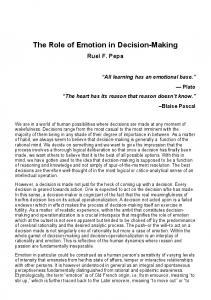
Sequential decision-making under uncertainty has been studied for decades. It is interesting to see that a huge segment of this field is covered by Markov models (Puterman, 1994). Indeed, the expressivity and the ease of modelization with those models make them very useful for solving such problems. Although they are all related, each Markov model requires different assumptions making it more suitable than the others in specific contexts. In this chapter, we review the most known and used models for sequential decision-making in stationary contexts. This will draw the outlines of a hierarchy of the models and let us look more closely to the part concerning non-stationary environments in the fourth section. We present the theoretical models along with the high-level ideas of some fundamental algorithms to solve the problems modeled with them. The hierarchy can be split in two types of models: the explanation models and the decision models. One purpose of explanation models is to represent an environment in order to understand its dynamics. On the opposite, decision models are used to compute the best action to perform considering the current situation in the environment (the current state). Of course, no decision can be made without a proper understanding of the problem. Therefore, each decision model is based on an underlying explanation model. Figure 1 sums up the relationships between the models that are presented in Chapters 2 and 3.

19

markov models for sequential decision-making

Explanation models Markov chain

extends

Semi-Markov chain extends

extends HMM derives MDP

extends

derives extends

HM-MDP

HSMM derives

equivalent

HS3MDP

extends MOMDP

extends

POMDP

Decision models Figure 1: Hierarchy of the main Markov models

1

Foreword

1.1 Markov Chains A Markov chain (Kemeny and Snell, 1960) allows us to formalize the evolution of the state of an environment whose dynamics are stochastic, i.e., dictated by probability distributions. Those distributions are also stationary, meaning that they do not change over time. When the evolution of an environment only depends on its current state, i.e., the condition of a probabilistic rule does not consider states that are further than one step before, it is said to fulfill the Markov property (Markov, 1954). When an environment fulfills the Markov property, is ruled by probability distributions and its current state is completely observable, all conditions are met to define a Markov chain for this environment. A Markov chain is characterized by a pair hS, T i with: • S, a finite set of completely observable states, • T : S → Pr(S ), a transition function over the states where T (s)(s0 ) is the probability of transitioning from s to s0 . Notation 1. Probabilistic functions. In this document, when defining and using functions like the transition function above, we use indifferently T (s)(s0 ) and T (s, s0 ) for concision purpose. Indeed, in this context, notations T : S → Pr(S ) and T : P S × S → [0, 1] are equivalent, as soon as s0 ∈S T (s, s0 ) = 1, ∀s ∈ S. We illustrate the Markov chain model with an elevator problem as below. 20

1 foreword

T (1f, 2f) T (1f, 1f)

1f

T (2f, 3f) 2f

3f

T (2f, 1f)

T (3f, 3f)

T (3f, 2f) T (2f, 2f)

Figure 2: Markov chain representation of the elevator problem

Example 2. Elevator problem. We consider an elevator in an office building with three floors named {1f, 2f, 3f}. At each floor, a user can call the elevator by hitting a button. Once inside, she can, like in any other elevator, choose the floor she wants to reach. The repartition of persons calling the elevator over the different floors depends on the time of the day. Indeed, in the morning, a majority of persons want to go up into their office rooms. On the opposite, at the end of the day, the persons want to go down and go home. During the day, variations may occur due to meetings or some external events. Note that, in order to be modeled, the problem needs to have a finite number of floors. Suppose we are only interested in representing the floor where the elevator is located. A Markov chain modeling this problem can be defined such that S = {1f, 2f, 3f} and T follows the distributions below: T (s, s0 )

1f

2f

3f

1f 2f 3f

0.8 0.2 0

0.2 0.6 0.1

0 0.2 0.9

We could also, assuming that all those components are observable, represent which buttons are pressed, which flow of persons (morning rush, evening rush, mid-day use) is currently occurring, etc. However, this means that the state space would be the Cartesian product of all the sets (floors, flows, buttons). For concision purpose, we choose to only represent the floors in this example. More visually, a Markov chain can be represented as a graph such as Figure 2. In this graph, nodes represent the states of the chain where 1f, 2f and 3f are the corresponding floors. An arc from node s to node s0 represents the transition between those states and thus is characterized by T (s, s0 ), the probability of transition presented above. Note that some transitions are not represented in the graph. They correspond to a probability of 0 in the table of probabilities and thus are impossible transitions. This model lets us easily represent a large class of problems. However, the most restraining hypothesis is the need to exactly observe the current state. This may not be suitable for problems like stock market forecasting, where we can observe the market trends but not the market internal state.

21


In order to relax this assumption, Baum and Petrie proposed the Hidden Markov Model (HMM) framework (1966), presented below. 1.2 Hidden Markov Models When using an HMM, the current state of the environment is not directly observable. Instead, an indirect observation is generated, conditioned by the current hidden state. An HMM is characterized by a tuple hS, T , O, Qi with: • S and T as in the Markov chain model, except S is not observable, • O, a finite set of observations, • Q : S → Pr(O ), an observation function. From state s, the next state s0 is drawn from T (s, ·) as in Markov chains. However, in HMMs, s0 is not directly observable. Instead, the agent receives an observation o drawn from Q(s0 , ·). Using the history of the observations, the agent can infer what is the underlying current state of the problem. As stated previously, Q(s0 , ·) is a notation equivalent to Q(s0 )(·). Example 3. Example 2 cont’d. Building upon the previous definition of this problem, we now consider that we want to represent what is the current flow of persons, using the knowledge of the current floor of the elevator. For this problem, the set of states is S = {morning, evening, mid-day}. This time, the current state s is not observable. Instead, we receive an observation o ∈ O = {1f, 2f, 3f}. T must be redefined to comply with the new definition of the problem: T (s, s0 )

morning

evening

mid-day

morning mid-day evening

0 0 0.9

0.9 0 0.1

0.1 1 0

The observation function Q may be defined as: Q ( s0 , o )

1f

2f

3f

morning evening mid-day

0.9 0.1 0.3

0 0.1 0.5

0.1 0.8 0.2

where Q(s0 , o) is the probability of observing o while arriving in state s0 . The interested reader can see Rabiner’s introduction (1989) for one of the most known introduction on HMMs.

22

2 sequential decision-making under uncertainty

1.3 Hidden Semi-Markov Models In some contexts, it is not realistic to consider that the state of the environment evolves at each timestep. To represent such problems, HMMs have been extended by considering that the current state of the problem can last several steps. This behaviour could be simulated in HMMs by setting a high probability of transition from a state to itself. However, this does not guarantee any minimum nor maximum number of steps stayed in this state. To account for such problems, Hidden SemiMarkov Models (HSMMs) have been proposed (Yu, 2010). In HSMMs, the transition function T needs to integrate the period of each state. This period is an element of D, a finite set of periods. Therefore, the new definition of the transition function is T : (S × D ) → Pr(S × D ). For instance, a transition from (s, 2) to (s0 , 4) means that, after 2 steps in state s, the environment stays in state s0 for 4 steps. Even though the current state of the environment stays the same for several steps, a (potentially different) observation is generated at each step. Example 4. Example 2 cont’d. As the different flows of persons are spread over a working day, it is relevant to consider they may last several steps. We keep the definition of S, O and Q as previously. Let us consider that the maximum period of time is 4 steps. The period for morning and evening flows is exactly 2 steps and may be 3 or 4 steps for the mid-day flow. We redefine T as follows: The transitions for impossible periods, e.g., ( morning, 1), are not represented in the morning

T

mid-day

evening

2

3

4

2

morning

2

0

0.5

0.4

0.1

mid-day

3 4

0 0

0 0

0 0

1 1

evening

2

0.8

0.1

0.1

0

table for clarity purpose. Markov chains, HMMs and HSMMs are fundamental for the explanation of Markov systems. However, we cannot formalize decision-making problems with them as they are only descriptive. Therefore, no decision can be taken into account when using these models. For this purpose, we have to rely on more evolved models presented in the following section.

2

Sequential decision-making under uncertainty

In this document, we are interested in an agent who is required to make several decisions sequentially. This agent has to take into account the current state of the environment (with complete or partial information) when making a decision and 23


executing an action as it will react according to this decision. This procedure has to be repeated infinitely or until the agent reaches her goal with an infinite horizon or up to a limited number of decision steps with a finite horizon. Depending on the assumptions made, the agent has different sets of information at her disposal to make decisions. Once the action has been made, the agent obtains a feedback from the environment signifying how good the chosen action was in the current state. The most famous model for sequential decision-making under uncertainty is the Markov Decision Process (MDP) model (Bellman, 1957). 2.1 Markov Decision Processes Markov Decision Processes extend Markov chains to decision-making problems. Indeed, like Markov chains, it is assumed that the current state of the system is exactly observed, the functions are stationary and the problem fulfills the Markov property. An MDP is defined by a tuple hS, A, T , Ri with: • S, a finite set of states, • A, a finite set of actions, • T : S × A → Pr(S ), a transition function over the states, • R : S × A → R, a reward function. Value T (s, a, s0 ) is the probability of reaching state s0 from state s after performing action a, and R(s, a) is the reward r ∈ R yielded by performing action a in state s. The reward function gives a feedback that can represent a payoff given to the agent. Alternatively, it can represent the preferences of the agent to some configurations of the environment. In any cases, this feedback, which can be a reward or a cost, is used to guide the decisions of the agent. As a side note, like Markov chains, an MDP can be seen as a graph whose vertices are the states of this MDP and arcs are the transitions between states. Figure 3 shows an example of a 3-state, 2-action MDP. To illustrate further the definition of an MDP, let us modify the elevator problem: Example 5. Elevator problem. An agent, possibly the elevator itself, now has to control the elevator over f floors in order, for the users, to wait the less possible amount of time. A decision in the context of this problem is a choice between moving the elevator of one floor up or down or to open the doors. As previously, at each decision step, a user may call the elevator at any floor and, once inside, select any desired floor to go. This time we also take into account the states of the buttons and the flows of persons. In this example, all components of the states are assumed to be directly observable. This decision problem can be formalized as an MDP where: • S = floors × button states × flows of persons, 24


(a1 , 0.5) (a1 , 0.5) s1

s2

( a1 , 1 )

(a1 , 0.9) (a1 , 0.1)

(a2 , 1)

a1

R s1 s2 s3

(a2 , 1)

s3

a2

s1

s2

s3

s1

s2

s3

-1 10 0

0.5 — —

— — -1

— — —

— — 10

— — —

(b) Reward table for the MDP

(a) Transition graph

Figure 3: Example of a 3-state, 2-action MDP with (action, probability) on arcs

• A = {up one floor, down one floor, open the doors}, • T can be any probability distribution preventing from going down when at floor 1 and going up at floor f while ensuring the elevator moves of only one floor, • R gives a negative feedback for each action that is not compliant with the destination of the users inside. To illustrate the reward function, say the elevator is at the second floor. It contains three persons, two of them want to go to the first floor and one to the third. In this configuration, if the elevator is going up, it complies with one the destination of one user while getting a negative feedback for each of the two others. In this definition of the problem, the uncertainty lies in the feedback given as the controlling agent does not know how many users want to go to a given destination. Once the problem is modeled, it needs to be solved. A solution of an MDP is a policy π, i.e., a sequence (δ0 , δ1 , . . . , δt , . . .) of decision rules such as each decision rule δt : S → A dictates which action to take for each state at timestep t. A policy π can be valued at timestep t by the expected discounted total reward it yields in state s: X V δt (s) = R(s, δt (s)) + γ T (s, δt (s), s0 ) × V δt+1 (s0 ) (1) s0 ∈S

where γ ∈ [0, 1[ is a discount factor. Function V δt , ∀t, is called the value function of π and Equation 1 is the Bellman equation of an MDP (Bellman, 1957). Solving an MDP consists in finding an optimal policy, i.e., a policy that maximizes the expected discounted sum of rewards:  

π ∗ (s) = arg max R(s, a) + γ a

X s0 ∈S

∗

 

T (s, a, s0 ) × V π (s0 )

(2)

Where arg maxa Fct(a) is the action a maximizing function Fct. Interestingly, the optimal policy of an MDP is stationary, i.e., for each timestep t, δt = δ0 . This property allows us to apply the same optimal policy, even if the number of decision steps goes to infinity. For instance, the optimal policy of the problem represented by Figure 3 is π ∗ (s1 ) = a1 , π ∗ (s2 ) = a2 , π ∗ (s3 ) = a2 . 25


The classical methods to exactly solve MDPs are the Value Iteration (Bellman, 1957) and the Policy Iteration (Howard, 1970) algorithms. However, both require full knowledge of the model. When the transition function and/or the reward function are not known, one can use reinforcement learning algorithms like Q-Learning (Sutton and Barto, 1998). This algorithm is guaranteed to converge to the optimal solution in a finite number of steps as soon as a discount factor γ < 1 is used when computing the value function (Watkins and Dayan, 1992). All these methods compute the optimal value function V ∗ iteratively. For the Value Iteration algorithm for instance, V ∗ is computed as the limit of the following sequence: V0 (0) = 0

(3)  X

Vi+1 (s) = max a 

s0

 

T (s, a, s0 )(R(s, a) + γVi (s0 )) , ∀i ≥ 1

(4)

The drawback of MDPs is that they require full knowledge of the current state. When the states are no longer observable but the decision-maker has partial information about the state of the system, one can rely on the Partially Observable Markov Decision Process (POMDP) model (Puterman, 1994). 2.2 Partially Observable Markov Decision Processes A POMDP is characterized by the tuple hS, A, T , R, O, Qi with: • S, A, T , R as defined for MDPs, • O, a finite set of observations, • Q : S × A → Pr(O ), an observation function In this model, after each action, instead of receiving the new state the agent is currently in, the agent receives an observation about this state. Note that the POMDP model is an extension of MDP. Indeed, an MDP is a POMDP where O = S and Q(s, a, o) = 1 if s = o and 0 elsewhere. In most problems, the observation function Q does not depend on the action taken. To reflect this simplification, when necessary the function will be defined as Q : S → Pr(O ). Recall that, as state previously, Q is also equivalent to S × O → [0, 1] as P soon as o∈O Q(s, o) = 1, ∀s ∈ S. Example 6. Partially observable elevator problem. Let us modify the previous formalization of the problem in order to comply with the POMDP framework. This model let us consider components that are not directly observed, like in HMMs. The modelization of the problem as a POMDP is as follows: • S = floors × buttons state × flows of persons, unobserved as in HMMs • A as previously, • T and R as previously but considering the new set of states, 26


o1

start

a1

o1

a3

o2

a2

o2 o1 o2

o2

a1

o1

Figure 4: Example of policy graph for a problem with at least 3 actions and 2 observations

• O = {1f, 2f, 3f}, • Q is defined considering the state and the action. Considering the set of observations, we can have an intuition on how to solve this problem. Indeed, if during a period of time, the observation 3f have been received a high number of times, we can deduce that the elevator is used most of the time to go up. To some extent, we could infer that the current flow is morning, when employees arrive at in building and go to their office room. Since the agent cannot observe the POMDP state, she has to choose the next action depending on the history of past observations. However, at step t, the probability distribution over the current state given the initial states and the history up to the current step t can be summarized by a probability distribution over states P (st |s0 , . . . , st−1 ) called belief state (Åström, 1965). Maintaining this distribution is sufficient and complete information to make optimal decisions. Therefore, a policy π can be considered as a mapping Pr(S ) → A. One can note that such a mapping cannot be computed in practice as the range of Pr(S) is infinite. Fortunately, a policy of a POMDP can be represented compactly as a policy graph (Hansen, 1997). This graph is a deterministic finite automaton where the nodes are the actions to perform and the transitions are the observations received. Figure 4 shows an example of a policy graph for a POMDP with at least 3 actions and 2 observations. In this graph, starting at the pointed node, the agent performs the action given by the label of the node. After receiving an observation from the environment (either o1 or o2 ), the agent needs to follow the corresponding arc in the automaton in order to transition to the next, possibly the same, node. She performs the action labeled by the node, and follows the arc corresponding to the new observation. Optimal algorithms have been proposed to solve POMDPs such as Witness (Kaelbling et al., 1998) and Incremental Pruning (Cassandra et al., 1997). They all use the property of the value function of the POMDP which is PieceWise Linear and Convex (PWLC). Therefore, the value function can be computed using the belief state 27


and value vectors called α-vectors. The problem of those exact algorithms is they do not scale to large-sized problems. Indeed, finding an optimal policy for infinitehorizon POMDPs is PSPACE-Complete (Papadimitriou and Tsitsiklis, 1987). For this situation, one can use appoximate algorithms such as SARSOP (Kurniawati et al., 2008) or Point-Based Value Iteration (Pineau et al., 2003). In various settings, some components of the state are fully observable while the rest of the state is not. It is the case, for instance, in multi-agent problems where the other agents are integrated in the environment. That way, the position of the decision maker is fully observable while the positions of the others are not. Ong et al. proposed the Mixed Observability Markov Decision Process (MOMDP) model (2010) to account for such problems. MOMDP algorithms exploit the mixed-observability property thus leading to a higher computational efficiency. 2.3 Mixed-Observability Markov Decision Processes An MOMDP is characterized by a tuple hSv , Sh , A, Ov , Oh , T , Q, Ri with: • Sv and Sh , respectively a set of the observable and of the hidden parts of the state, • A, a finite set of actions, • Ov and Oh , respectively a finite set of observations on the visible and and on hidden parts of the state, with Ov = Sv , • T : Sv × Sh × A → Pr(Sv × Sh ), a transition function, • Q : Sv × Sh × A → Pr(Ov × Oh ), an observation function, • R : Sv × Sh × A → R, a reward function. Note that an MOMDP is a structured POMDP hS, A, T , R, O, Qi where S = Sv × Sh and O = Ov × Oh . Example 7. Mixed observable elevator problem. In a more realistic setting, the state of the buttons and the current floor are observable while still being part of the current state. However, the current setting of the flow of persons cannot be observed, only the number of persons induced by the flow can be. In this situation, the MOMDP modelization of this problem is: • Sv = floors × buttons states, • Sh = flow sides, • A, as previously, • Ov = floors × buttons states, • Oh = {0 persons, 1 person, . . . , n persons}, • T , Q and R set according to the MOMDP formalization. 28

3 partially observable monte-carlo planning

The different algorithms proposed to solve MOMDP modeled problems extend standard POMDP algorithms in order to exploit the structure of this model. In Mixed-Observability Incremental Pruning (MO-IP), Araya-López et al. (2010) used the structure of MOMDPs to lower the dimension of the hyperplans (the α-vectors with more than 2 states) characterizing the value function. With this reduction, the set of regions (the belief state intervals associated to the action performing the best on this interval) contains less elements thus allowing to tackle bigger instances while keeping the optimality of the solution. When the problem cannot be solved due to its size, Mixed-Observability SARSOP (MO-SARSOP) (Ong et al., 2010) can be used to some extent. In fact, MO-SARSOP is an algorithm on MOMDPs in which we can plug in most of the POMDP algorithms. The factorization permitted by MOMDPs allows us to represent the whole belief space with a union of lower-dimension belief spaces (particularly on the observable part and on the non-observable part). With this separation, at each iteration of the algorithm, a POMDP algorithm can be applied on the subspace representing nonobservable part (SARSOP in this case). In the same iteration, two sets of α-vectors (the different pieces of the PWLC value function) are computed and updated on the subset of the observable part: one representing a lower-bound on the optimal value function and one representing an upper-bound. Finally, after enough iterations, the lower-bound approximation converges towards the optimal value function. For both POMDPs and MOMDPs, when no other solution is able to cope with high-dimension problems, we can resort to Monte-Carlo methods like POMCP presented below.

3

Partially Observable Monte-Carlo Planning

The Partially Observable Monte-Carlo Planning (POMCP) algorithm (Silver and Veness, 2010) is one of the most efficient online algorithms to approximately solve large-sized POMDPs. To choose an action at a given timestep, POMCP (Algorithm 1) runs an effective version of Monte-Carlo Tree Search (MCTS) (Coulom, 2007), called UCT (Upper Confidence Bounds (UCB) applied to Trees) (Kocsis and Szepesvári, 2006), using a black-box simulator of the environment and a particle filter to approximate a belief state. Each particle of the filter represents a state of the POMDP being solved. Therefore, with an infinite-sized filter, the particle repartition would exactly match the belief state of the POMDP. The necessity to have a simulator can seem to be highly constraining but all algorithms presented previously, at the exception of Q-Learning, require to know exactly the model. Therefore, a simulator is a relaxation of this constraint. Moreover, it does not require to reflect exactly the real environment, at the cost, of course, of a less optimal solution. POMCP uses the simulator to run a fixed number of simulations in order to evaluate the actions before performing, in the real environment, the best action found in the search tree. At one decision step, to choose which action to perform, search(τ ) 29


root

a1

o1

o2

...

a2

...

o|O|

o1

o2

...

a|A|

o|O|

Figure 5: Full tree created by POMCP for a depth of 1 if all observations are received

is invoked with the current history τ , i.e., the sequence of past observations and actions. This history can be expanded with an action a giving τ a and an observation o giving τ ao. The root of the search tree is a node matching the last seen observation in the real environment. Its children are all possible actions, whose own children are the experimented observations during the simulations of the action. Figure 5 represents a full search tree at a depth of 1. A node of the tree is a triplet hN (τ ), V (τ ), B (τ )i associated to τ where the components are respectively the number of times τ has been visited, its mean value and the set of particles (i.e., POMDP states) for this history. During a simulation, the algorithm randomly draws a particle p from the particle set B (τ ) and uses the simulator G (p, a) to get the new particle p0 , the observation o and the reward r. Of course, the particle p0 is a state of the POMDP such that T (p, a, p0 ) 6= 0. Actions are selected (Line 19 of Algorithm 1) following the UCB1 (Auer et al., 2002) procedure guaranteeing a good exploration-exploitation compromise. Once all simulations have been done, a step is performed in the real environment with the action returned by search, i.e., the best action found in the search tree. The algorithm sets the new root to the node matching this observation and prunes the tree to only keep nodes that are descendant of the new root. At the beginning, POMCP is initialized with an empty history and an initial (e.g., uniform) distribution I over states. Two important parameters have to be set to guarantee that a good action is selected: the tree depth and the number of simulations. The tree depth d can be deduced from the discount factor γ for a given precision > 0 as follows: d = blog()/ log(γ )c. The depth value is set such that each step deeper than d yields a payout small enough to be neglected, due to the discount factor. That way, the simulation part of the algorithm is sure to terminate in a finite time. The higher the number of simulations, the better the estimation of the values of the actions but the longer it takes to run. This parameter is generally determined by time constraints. However, as the number of simulations tends to infinity, this algorithm is theoretically guaranteed to choose the optimal action at each step. Finally, notice that the size of the initial particle filter is generally set in function of the number of simulations. 30

3 partially observable monte-carlo planning

Algorithm 1: POMCP 1 2 3 4 5 6 7

procedure search(τ ) foreach simulations do if τ = empty then p∼I else p ∼ B (τ ) simulate(p, τ , 0) return arg max V (τ b) b

8 9 10 11 12

13 14 15 16 17 18

procedure rollout(p, τ , depth) if γ depth < then return 0 a ∼ πrollout (τ , ·) (p0 , o, r ) ∼ G (p, a) return r + γ.rollout(p0 , τ ao, depth + 1) procedure simulate(p, τ , depth) if γ depth < then return 0 if τ ∈ / T ree then forall a ∈ A do T ree(τ a) ← (Ninit (τ a), Vinit (τ a), ∅) return rollout(p, τ , depth) q

19

a ← arg max V (τ b) + c log (N (τ ))/N (τ b) b

20 21 22 23 24 25 26

(p0 , o, r ) ∼ G (p, a) R ← r + γ.simulate(p0 , τ ao, depth + 1) B (τ ) ← B (τ ) ∪ {p} N (τ ) ← N (τ ) + 1 N (τ a) ← N (τ a) + 1 V (τ a) ← V (τ a) + (R − V (τ a))/N (τ a) return R

31


4

Non-stationary environments

While POMCP can help to tackle high-dimension problems, one of the main limitations of the (MO/PO)MDP framework is that it requires the transition and reward functions to be stationary. Without this condition, the algorithms previously presented lose their optimality, convergence guarantee or performance guarantee. In the context of sequential decision-making under uncertainty, a stationary environment is an environment whose components do not evolve over time. For instance, for an MDP, this concerns the sets of states and actions but it also means that the transition probabilities never change and the reward function remains the same. Example 8. Example 2. If we illustrate the notion of stationarity on the elevator problem, the set of states and actions must remain identical over time. This means that, for instance, no elevator, no new floor can be added and no new move can be performed. Likewise, the transition and reward functions cannot be modified over time, meaning that users always react identically to the elevator and its behaviour never changes. Unfortunately, the stationarity hypothesis does not hold in problems like stock market forecasting, multi-agent problems where agents learn simultaneously or the previously presented elevator problem. We now introduce methods able to model and solve non-stationary decision-making problems. Those methods are as diverse as the different types of non-stationarity. Among them, two types of methods are prominent: regret-based and Markov methods. The following section presents regret-based methods as an introduction, although we will not use them in our contributions. 4.1 Regret minimization The main purpose of regret minimization methods is to relax the assumptions of stationarity and stochasticity. Removing the latter let us represent problems where the evolution of the environment can be dictated by another agent, possibly an opponent. In such a case, the environment is said to be adversarial. Such problems are clearly non-stationary as the opponent can modify her strategy in order to adapt to the decision-making agent and thus may modify the dynamics of the environment. In regret minimization, the agent is facing a two-players repeated game, i.e., a problem where two agents (the player and the opponent, which can be the environment) choose an action to play, get a feedback (a reward or a cost) and repeat the game (see, for instance, (Cesa-Bianchi and Lugosi, 2006, Chapter 7)). In this context, the regret is the difference between the feedback of the optimal action and the feedback of the action played. The agent thus tries to minimize the regret a posteriori in the repeated game, i.e., minimize the difference between her policy and a reference policy. Of course, this reference policy is not known a priori and thus cannot be executed. More formally, let π be the policy of player p, π 0 the reference policy and lπt (respectively lπt 0 ) the cost in [0,1] yielded by π (respectively π 0 ). 32

4 non-stationary environments

We can compute LTπ = Tt=1 lπt and LminT = Tt=1 lπt 0 , the sums of costs for each policy. Finally, RπT = LTπ − LminT is the regret at timestep T of policy π. The objective is thus to find the policy π minimizing RπT (Nisan et al., 2007, Chapter 4). P

P

There exists several methods minimizing the regret under different assumptions (see, for instance, (Nisan et al., 2007; Cesa-Bianchi and Lugosi, 2006; Bubeck and Cesa-Bianchi, 2012)). Those methods are quite efficient in the general case and generate a sub-linear regret comparing to the best policy a posteriori. Moreover, the mean regret tends to 0 with the number of steps increasing. While this is a very interesting framework to tackle problems with a non-stationary environment, those methods are pessimistic as they consider the worst case scenario. Recently, Neu (2013) worked on such methods on non-stationary MDPs. This is an efficient starting point for the interesting reader as we do not investigate more deeply those methods in this document. 4.2 Hidden-Mode Markov Decision Processes Besides those regret-based methods, works have been done in the context of Markov models to represent non-stationary problems. In particular, Choi (2000) proposed an interesting hypothesis using the concept of modes. In this work, the nonstationarity is limited to a number of stationary settings, called modes or contexts, between which the environment can switch. Example 9. Example 2 cont’d. In the elevator problem, the different flows of persons (morning-rush, evening-rush, general activity) can be represented as modes. If all the other parameters (like the current state) are integrated into a known transition function, we can consider the environment stationary if the flow side is fixed. Therefore, the non-stationarity comes from the evolution of this flow through the time and thus of the current mode. Choi et al. proposed the Hidden-Mode Markov Decision Process (HM-MDP) model to formalize this subclass of non-stationary problems (2001). The environmental changes are limited to a fixed and known number n of modes. Each mode represents a possible stationary environment, formalized as an MDP. Transitions between modes represent environmental changes. Note that there is no assumption about the variability of the changes between modes. This means that the differences in the functions for each mode can represent either smooth or abrupt changes. Restraining the changes to stationary modes may seem to highly limit the range of problems that can be addressed but, in fact, every non-stationary environments whose evolution is stochastic, can be modeled by an HM-MDP with a high enough number of modes. The extreme case being an infinite number of modes, one for each decision step. As for the probabilistic functions, one can imagine that the set of the states and the set of actions could evolve as well. In such a case, it is sufficient to define the global set of states as the union of the set of states of each mode. It is identical for the set of actions. 33


m1

s’

m2

C ( m2 , m1 )

0

s0 0

Tm1 (s, a, s )

Tm2 (s, a, s )

s

s

C ( m1 , m2 )

C ( m1 , m1 )

C ( m2 , m2 )

Figure 6: HM-MDP representation with 2 modes and 4 states

Formally, an HM-MDP is defined by a tuple hM , Ci as follows: • M = {m1 , . . . , mn }, a finite set of modes where mi = hS, A, Ti , Ri i, i.e., an MDP, • C : M → Pr(M ), a transition function over modes. Note that S and A are shared by all mi ’s and that an HM-MDP with n = 1 is a standard MDP. In HM-MDPs, the only observable information is the current state s ∈ S. The current mode m ∈ M is not observable. Figure 6, showing a 2-mode, 4-state HM-MDP, depicts how HM-MDPs can be visualized. In order to illustrate the HM-MDP formalization, let us modify and make the elevator problem more precise. Example 10. Elevator problem with hidden modes. Consider a fixed number e of elevators to control in a building with f-floors. The flows of persons are no longer part of the states. Indeed, with HM-MDP, they are modeled as modes and thus are not required to explicitly belong to the states. The number of states of the HM-MDP is then 2f (e+1) × f e . The actions are left untouched, leading to an action set of size 3e . Finally, in this problem, the reward function is identical as previously. Considering an office building of 2 floors with 1 elevator: • M = {morning, evening, mid-day}, • S = {1st floor call button states} × {2nd floor call button states} × {1st floor drop-off button states} × {2nd floor drop-off button states} × {elevator positions} • A = {open, up, down}, as previously defined

34

5 conclusion

In this small example, there are 32 states, 3 actions and 3 modes. The transition function in the morning rush-hour mode describes the situation where it is more probable for the elevator to be called at the first floor. In the late-afternoon rushhour mode, it describes the opposite situation where users tend to leave the office. For the non-rush-hour mode, the transition function models the normal operating situation. Choi et al. have shown that an HM-MDP can be seen as a POMDP hS, A, T , R, O, Qi where: • S = M × S, • A = A, • T (hm, si, a, hm0 , s0 , i) = Tm (s, a, s0 ) × C (m, m0 ), • R(hm, si, a) = Rm (s, a), • O = S, • Q(hm, si, a, o) = 1 if s = o and 0 otherwise. Choi et al. have also proposed some algorithms to optimally solve HM-MDPs (Choi, 2000; Choi et al., 2001). They adapt exact POMDP solving methods in order to exploit the structure of HM-MDPs. Those adapted methods can solve larger instances of HM-MDPs than the original ones, but they may still suffer from the curse of dimensionality. Like exact POMDP solving algorithms, exact HM-MDP solving algorithms do not scale. In that case, one has to resort to approximate algorithms like POMCP.

5

Conclusion

This chapter presents an overview on models and algorithms addressing sequential decision-making problems under uncertainty. In all the original works we propose in the remaining of this document, we focus on the subclass of problems assumed to be in non-stationary environments. In particular, HM-MDPs seem very suitable as they can theoretically model a large class of non-stationary environments. However, some hypothesis are too strong. In Chapter 3, we remove some assumptions and propose a new model called HS3MDP, that we will reuse in Chapter 8.

35

SEQUENTIAL DECISION-MAKING IN N O N - S TAT I O N A RY E N V I R O N M E N T S This chapter is based on a work published in (Hadoux et al., 2014b). 1

2

3

4

Hidden Semi-Markov-Mode MDP . . . . . . . 1.1 Definition . . . . . . . . . . . . . . . . 1.2 Discussion . . . . . . . . . . . . . . . . Solving an HS3MDP . . . . . . . . . . . . . . 2.1 Adaptation to the structure . . . . . . 2.2 Exact representation of the belief state Experimental results . . . . . . . . . . . . . . . 3.1 Traffic light . . . . . . . . . . . . . . . 3.2 Sailboat . . . . . . . . . . . . . . . . . 3.3 Elevators . . . . . . . . . . . . . . . . 3.4 Randomly generated environments . . Conclusion and discussion . . . . . . . . . . .

. . . . . . . . . . . .

. . . . . . . . . . . .

. . . . . . . . . . . .

. . . . . . . . . . . .

. . . . . . . . . . . .

. . . . . . . . . . . .

. . . . . . . . . . . .

. . . . . . . . . . . .

. . . . . . . . . . . .

. . . . . . . . . . . .

. . . . . . . . . . . .

. . . . . . . . . . . .

. . . . . . . . . . . .

. . . . . . . . . . . .

38 38 39 40 41 41 42 42 44 45 46 47

We have seen in the previous chapter that some types of non-stationary environments can be modeled with an HM-MDP. However, with this model, the environmental changes are described by a Markov chain and thus occur at each decision step. We argue that this assumption is not always realistic. Indeed, in the elevator problem for instance, allowing, even with a small probability, the environment to be able to change between different rush modes at every move of the elevator is debatable. In this chapter, we propose a natural extension of HM-MDPs, called Hidden SemiMarkov-Mode Markov Decision Processes (HS3MDPs), where the non-stationary environment evolves according to a semi-Markov chain. This new model is to Hidden Semi-Markov Models (Yu, 2010) what HM-MDPs are to Hidden Makov Models. In HS3MDPs, when the environment stochastically changes to a new mode, it stays in that mode during a stochastically drawn duration. While HM-MDPs assume that environmental changes follow a geometric law, this assumption is relaxed in HS3MDPs. In order to solve large-sized HS3MDPs, we exploit the POMCP algorithm previously described in Section 3 of Chapter 2. We present two improvements of POMCP for solving HS3MDPs more efficiently. The first adaptation exploits the special structure of HS3MDPs and the second furthermore represents belief states exactly instead of using particle filters. Finally, we experimentally validate those algorithms showing their effectiveness on a diverse range of domains.

37

3

sequential decision-making in non-stationary environments

1

Hidden Semi-Markov-Mode MDP

The HM-MDP framework is not always the most suitable model for representing sequential decision-making in non-stationary environments as it assumes that the environment may change at every timestep. For instance, modeling the elevator problem with an HM-MDP is problematic as decisions have to be made every (say) second, while a mode (rush hour or not) can last several hours. In a problem where this assumption does not hold, the usual modeling trick is to set a low probability of transition between modes. However, from a theoretical viewpoint, this is more than questionable when mode transitions are not geometrically distributed. The first contribution of this document is to propose a more natural model for such cases where the environment dynamics evolve according to a semi-Markov chain. 1.1 Definition Formally, a Hidden Semi-Markov-Mode MDP (HS3MDP) is defined by a tuple hM , C, Hi where: • M and C are defined as for HM-MDPs, • H : M × M → Pr(N) is a mode duration function. Transition C (m, m0 ) represents the probability of moving to new mode m0 from current mode m knowing that the duration in m (i.e., the number of remaining timesteps to stay in m) is null. Value H (m, m0 , h) represents the probability of staying h timesteps in the new mode m0 when the current mode is m. Both the mode and the duration are not observable. Note that, it is not always relevant for the duration function to take into account the previous mode. For this purpose, the duration function may be specified as H (m0 , h), equivalent to H (m, m0 , h), ∀m ∈ M . At each timestep, after a state transition in current mode m, the next mode m0 and its duration h0 are determined as follows: if h > 0 m0 = m, h0 = h − 1,  if h = 0 m0 ∼ C (m, ·),    h0 = k − 1 where k ∼ H (m, m0 , ·)     

(5)

where h is the duration of current mode m. If h is positive, the environment dynamics do not change. But, if h is null, the environment moves to a new mode according to the transition function C and the number of steps to stay in this new mode is drawn following the conditional probability H. Example 11. Elevator problem with semi-Markov hidden modes. We can extend the HM-MDP modelization of the elevator problem to an HS3MDP: • M , S and A, as defined for the HM-MDP, • H can be defined as follows:

38

1 hidden semi-markov-mode mdp

H (m, h)

0

1

2

3

4

morning evening non-rush

0.2 0.1 0

0.2 0 0

0.6 0.2 0

0 0.4 0.2

0 0.3 0.8

where {0, . . . , 4} are the number of decision steps to stay in the current mode before considering an environment change. This definition of the duration function can be interpreted as follows: Morning rush-hours usually do not last as people tend to arrive at the same time (hence the duration between 0 and 2). On the opposite, evening rush-hours may last longer and are more spread. We can ensure that no evening rush can occur consecutively by setting C(evening, evening) = 0. Finally, as non-rush hours are between the two other modes, they last longer with a high probability. Like HM-MDPs, HS3MDPs form a subclass of POMDPs. An HS3MDP can be reformulated as a POMDP hS, A, T , R, O, Qi whose components are defined by: • S = M × S × N, • A = A, • T (hm, s, hi, a, hm0 , s0 , h0 i) = αTm (s, a, s0 ) with:

C (m, m0 ) × H (m, m0 , h0 ) if h = 0, α =  1 if h0 = h − 1 and m0 = m,  0 otherwise   

(6)

• R(hm, s, hi, a) = Rm (s, a), • O = S, • Q(hm, s, hi, a, o) = 1 if s = o and 0 otherwise. 1.2 Discussion It is easy to show that HM-MDPs form a subclass of HS3MDPs. In fact, a problem represented as an HS3MDP can also be exactly represented as an HM-MDP by augmenting the modes. The two models are thus equivalent in the following sense. Definition 1. Model equivalence. A model M is expressively equivalent to a model M0 if and only if a problem that can be represented in model M can also be exactly represented in model M0 and vice-versa. Proposition 1. HM-MDPs are equivalent to HS3MDPs. Proof. ⇒ Given an HM-MDP, we can define an equivalent HS3MDP by setting a mode duration function H such that ∀m, m0 , H (m, m0 , 1) = 1 and H (m, m0 , h) = 0, ∀h 6= 1. At each timestep, h = 0, thus leading only to the first alternative of Equation 6. This turns out to be the exact formulation of an HM-MDP. 39


⇐ Given an HS3MDP, we show how to build an equivalent HM-MDP. To that aim, we build a sequence of equivalent HS3MDPs. Denote hM1 , C1 , H1 i the initial HS3MDP. We repeat the following operation to build the sequence: If, for hMi , Ci , Hi i, there exist m, m0 ∈ Mi and h 6= 1 such that Hi (m, m0 , h) > 0, we define the next HS3MDP hMi+1 , Ci+1 , Hi+1 i as follows: Mi+1 = Mi ∪ h0 6=1 {m00 , . . . , m0h0 −1 |Hi (m, m0 , h0 ) > 0} Ci+1 (m, m0h0 −1 ) = Ci (m, m0 ) × H (m, m0 , h0 ) Ci+1 (m0j , m0j−1 ) = 1, ∀j > 0 Ci+1 (m1 , m2 ) = Ci (m1 , m2 ), ∀(m1 , m2 ) 6= (m, m0 ) Hi+1 (m, m0h0 −1 , 1) = Hi+1 (m0j , m0j−1 , 1) = 1, ∀h0 > 0, j > 0 Hi+1 (m1 , m2 , h0 ) = Hi (m1 , m2 , h0 ), ∀(m1 , m2 ) 6= (m, m0 ), ∀h0 S

(7)

where for all j, m0j is a duplicate of m0 and Ci+1 and Hi+1 are null for the unspecified cases. When this operation cannot be iterated, in the last HS3MDP, unreachable modes can be removed. Finally, the resulting HS3MDP corresponds to an equivalent HM-MDP. Although HM-MDPs and HS3MDPs are proven to be equivalent, representing HS3MDPs in such a way feels unnatural and leads to a higher number of modes, which moreover, would have a negative impact on the solving time. It is also obvious that, if the maximum duration is unbounded, the equivalent HM-MDP would have an infinite number of modes, making it difficult to solve. Interestingly, HM-MDPs and HS3MDPs are also MOMDPs. Indeed, with the state being observable and the mode (as well as the duration for HS3MDPs) being not, the two models can easily be transformed into a MOMDP. This enable us to use adapted algorithms for MOMDPs, which are more efficient than their POMDPs counterparts in this context. However, we choose to base our solving method on POMCP, because it tends to be more efficient than specialized algorithms on MOMDPs and more generally on factored POMDPs, even when POMCP is run using non-factored representations (Silver and Veness, 2010).

2

Solving an HS3MDP

As for POMDPs, solving problems modeled with HS3MDPs is a difficult task to address. In their work, Chadès et al. (2012) proposed the hidden-model MDP model or hmMDP (note the lower case) and proved that finding an optimal policy in a hmMDP is a PSPACE-complete problem. Independently discovered, hmMDPs turn out to be a subclass of HM-MDPs where there the mode, once selected, cannot be changed. As finding an optimal policy for a POMDP is also a PSPACE-complete problem (Papadimitriou and Tsitsiklis, 1987), both HM-MDPs and HS3MDPs, as they are equivalent, are PSPACE-complete to solve. In order to be able to tackle large instances of problems, we therefore focus on an approximate solving algorithm. A first naive approach is to apply POMCP to directly solve the POMDP derived from an HS3MDP. In that case, a particle in 40

2 solving an hs3mdp

POMCP represents a mode m, a state s and a duration h of the HS3MDP. We propose in this section two possible improvements to this naive approach. Notice that, as a subclass of HS3MDPs, these solving methods can also be applied to HMMDPs. 2.1 Adaptation to the structure In large instances, POMCP can suffer from a lack of particles to approximate the belief state, especially if the number of states in the POMDP and/or the horizon are large. To tackle this issue, a particle reinvigoration technique is used in the original algorithm. However, it is often insufficient. When POMCP runs out of particles, it samples the action set according to a uniform distribution, which obviously leads to suboptimal decisions. We propose a first adaptation of POMCP that exploits the structure of HS3MDPs to delay the lack of particles. In fact, in the derived POMDP, as the agent observes a part of the state of the POMDP, a particle needs only to represent non-observable information, that is, the mode m and the duration h. This adaptation allows us to initially distribute the same amount of particles over a set whose cardinality is much smaller. However, the size of the particle set |B (τ )| still depends on the number of simulations. This modification of POMCP is introduced at line 3 of Algorithm 1. 2.2 Exact representation of the belief state When solving large-sized problems, the above adaptation of POMCP may still suffers from lack of particles. We thus propose a second adaptation where we replace the particle set B by an exact representation of the belief state. This representation consists of a probability distribution µ over M × N (modes and duration in the current mode). Lines 3 and 5 of Algorithm 1 are modified as particles are now drawn according to a probability distribution. Line 22 is not needed anymore. This probability distribution is updated after a new observation using the following equation: µ0 (m0 , h0 ) =

1 T 0 (s, a, s0 ) × µ(m0 , h0 + 1)+ K m X C (m, m0 ) × Tm (s, a, s0 ) × µ(m, 0) × H (m, m0 , h0 + 1)

(8)

m∈M

where K is the normalization term and elements s, s0 , a are respectively the previous observation, the new observation given by the real environment and the action performed and given by the procedure search. This update is performed after every action executed in the real environment. In HM-MDPs we can rewrite the above equation knowing µ(m0 , h0 + 1) = 0, ∀m0 , h0 and H (m, m0 , 1) = 1. We then obtain: µ0 ( m 0 ) =

1 X C (m, m0 ) × Tm (s, a, s0 ) × µ(m) K m∈M

(9)

41


We recover to the HM-MDP update equation described by (Choi et al., 2000). Unlike the previous adaptation, the spatial complexity of this one does not depend on the number of simulations. Indeed, µ is a probability distribution over M × N. Assuming a finite maximum duration hmax , which is often the case in practice, there always exists a number of simulations N for which the size of the particle set is greater than the length of this distribution. In such a case, this second adaptation will be more interesting to consider. The time complexity of the update of the exact representation is O (|M | × hmax ). It is to be compared to the particle invigoration of the original POMCP combined with the first adaption which is O (N ) with N being the number of simulations.

3

Experimental results

We tested POMCP and our two adapted versions on four non-stationary problems. The first three environments are problems from the literature (Choi, 2000). We solved an extended version of each problem modeled as an HS3MDP. Recall that those adapted versions of the problems cannot be represented as efficiently with HM-MDPs (see the discussion related to Proposition 1). The code used for those experiments can be found on Github1 . H (m, m0 , ·) is defined as a truncated Gaussian probability distribution on duration h of the mode m0 after a transition from m. The mean of the Gaussian is uniform randomly drawn between 1 and 5 when creating the environment. The standard deviation is set such as when the mean is located in the middle of the interval, each duration can be drawn. We present the results for the original POMCP and for our adaptations of POMCP: the Structure Adapted (SA) and Structure Adapted combined with the Exact Representation (SAER) of belief states. We also show the results of the optimal policy when it could be computed, using Cassandra’s POMDP toolbox2 and MO-IP (ArayaLópez et al., 2010). We also used MO-SARSOP (Ong et al., 2010) with one hour of policy computation time when the model could be generated for offline computing. We present the performances of the algorithms for several numbers of simulations to study how the quality of the solutions evolves. For each number of simulations we averaged the cumulative discounted rewards over 1000 runs. We reported results that could be obtained within one hour on a computer equipped with an Intel XeonX5690 4.47 Ghz core and 16G of RAM. We chose to present the raw results for the original POMCP and percentages for the others. Reported percentages correspond to the percentages of improvement brought by our modified versions. 3.1 Traffic light In the traffic light problem depicted in Figure 7, the environment is a two-way road where the system has to choose which side to let pass. It has to decide which traffic light to switch on, knowing only the current state of the lights and the presence 1 https://github.com/EHadoux/HS3MDP 2 http://www.pomdp.org/code/index.html

42

3 experimental results

Figure 7: Traffic light problem (courtesy of T. Huraux)

or not of cars on each side of the road. In this problem, the HS3MDP has two modes: rush on the left or on the right and two actions to choose which light to switch on. The model contains eight states depending on the light state and on the presence or not of cars on the left and on the right. The reward function gives a negative reward when a car waits on a side of the road whose light is shut off. When the duration hits 0, the environment has a probability of 0.9 to stay in the same mode and 0.1 to change. The transition function over the state depends on the probability of cars arriving on each side, according to the current mode. Finally, the duration function is defined as stated previously. Exact probabilities for the original problem can be found in (Choi, 2000) except the duration function H which is a Gaussian bell whose mean is drawn between 1 and 5. Table 1 describes results for the traffic light problem, using different algorithms: original POMCP, Structure Adapted (SA), Structure Adapted combined with Exact Representation of belief states (SAER) and Finite Grid, MO-IP and MO-SARSOP. The last three algorithms yield the same results, which are presented in column “Optimal” to give an idea of the optimal value. The performances of the original POMCP almost strictly increase with the number of simulations. They therefore get closer to the optimal value, which translates into decreasing percentages in Column “Optimal” of Table 1. Since our modified versions of POMCP performs better than the original one (positive percentages for columns “SA” and “SAER”), they also get closer to the optimal. For instance, with 512 simulations, 4.7% of improvement for SAER compared to 9.3% for Column “Optimal” means that the performances of SAER are half-way between those of the original POMCP and the optimal value. Note that a decreasing percentage does not mean a raw decrease in the performances. 43


Simulations 1 2 4 8 16 32 64 128 256 512 1024 2048

Original

SA

SAER

Optimal

-3,42 -2,86 -2,80 -2,68 -2,60 -2,45 -2,47 -2,34 -2,41 -2,32 -2,31 -2,38

0.0% 3.0% 8.1% 6.0% 8.0% 5.3% 10.0% 4.3% 8.5% 5.6% 5.1% 9.0%

0.0% 4.0% 8.8% 9.4% 8.0% 6.9% 9.1% 3.4% 10.5% 4.7% 7.0% 10.5%

38.5% 26.5% 25.0% 21.7% 19.2% 14.3% 14.9% 10.4% 12.7% 9.3% 9.3% 11.8%

Table 1: Results for traffic light

It means that the increase of the performances of the original POMCP is higher than those of the other algorithms. Nonetheless, the percentages being positive, the latter still perform better. Theoretically, POMCP converges towards the optimal solution as the number of simulations increases. Experimental results (Table 1) show that it is also the case for our adapted versions whose performances are always at least as good as the original POMCP. In the traffic light problem, both adaptations of POMCP are roughly similar. In fact, the size of the problem is quite small so the original POMCP and the structured adapted POMCP do not run out of particles. Moreover, there are enough particles to draw a high quality estimation of the belief state. That is why, the exact representation of belief states does not significantly outperform other POMCP versions. Nonetheless, our adaptations of POMCP both outperform the original version since exploiting the structure of the HS3MDP leads to more accurate belief states. 3.2 Sailboat The sailboat problem, depicted in Figure 8, is about controlling a boat from a corner of a finite grid to the opposite corner. The states are possible positions in the grid and the modes are the different wind directions, limited to North, South, West and East. Two possible actions manage the sail orientation between North-South and East-West. The transition function over states depends on the sail orientation given the wind direction. If the sail is well-oriented the boat goes towards the wind direction with a small probability to derive (0.1 on each side). Otherwise, the boat does not move. The environment has a probability of 0.5 to stay in the same mode, 0.2 to go to an adjacent one and 0.1 to go to the opposite one when the duration is at 0. The duration function is defined as previously. The reward function gives a

44


Figure 8: Sailboat problem (courtesy of T. Huraux)

reward of 1 when the goal is reached. This problem can be enlarged as needed by increasing the size of the grid. Results for a 7 × 7 grid are reported in Table 2. Due to probabilities of transition between modes, the environment can stay several steps in the same mode thus leading to the same wind direction. When the boat is on an edge of the grid, it cannot move until the wind changes to a more favorable configuration. This particularity of the environment leads to a big set of runs where the boat cannot reach the goal and gets stuck on an edge until the end of the run. Moreover, the small drops in the original POMCP performances can be explained with the low number of simulations. If this number is not high enough to explore efficiently, the impact of the randomness can lead to a high variance. Results show that our adaptations always perform better than the original method and that SAER performs almost always better than SA. We also can see that SAER converges towards the optimal results as the number of simulations increases. 3.3 Elevators In the elevator problem shown in Chapter 2, the environment can stay in the current mode (see Example 11 above) with a probability of 0.1 and has a probability 0.45 to change to the other two when the duration is null. The duration function is the same than for the previous experiments. Table 3 contains results for an instance with 7 floors and 1 elevator whereas Table 4 shows results for an instance with 4 floors and 2 elevators. We were not able to compute the optimal policy for these instances because of their large sizes. We can see that, for this application, the performance of both adaptation are roughly similar.

45


Simulations 1 2 4 8 16 32 64 128 256 512 1024 2048 4096 8192

Original

SA

SAER

MO-SARSOP

60 63 55 70 59 66 90 94 119 159 177 206 226 227

11.7% 30.2% 38.2% 8.6% 13.6% 28.8% 21.1% 53.2% 48.7% 31.4% 20.9% 13.6% 12.4% 20.7%

6.7% 30.2% 54.5% 27.1% 88.1% 92.4% 45.6% 71.3% 76.5% 27.0% 28.8% 10.2% 16.4% 25.6%

408.3% 384.1% 454.5% 335.7% 416.9% 362.1% 238.9% 224.5% 156.3% 91.8% 72.3% 48.1% 35.0% 34.4%

Table 2: Results for sailboat (7×7 grid) Simulations

Original

SA

SAER

-10.56 -10.60 -10.50 -10.49 -10.44 -10.54

0.0% 0.0% 2.2% 4.2% 5.2% 6.2%

1.1% 0.0% 3.6% 3.9% 5.0% 6.2%

1 2 4 8 16 32

Table 3: Results for elevator (f = 7, e = 1)

In fact, the SAER adaptation shows its efficiency when the original POMCP and the SA adaptation runs out of particles. For those problems, the number of simulations is not high enough to lead to particles deprivation. However, it is important to note that our methods always outperform the original POMCP whose performances increase with the number of simulations and converge to the optimal solution. The low number of simulations reached during the computation time is explained by the representation of the transition function. In this problem, transitions are not represented by a matrix of probabilities because of the high number of state components. The transitions are based on a set of rules (allowing, among other things, to process the change of floor of each elevator independently), leading to a longer computation time. 3.4 Randomly generated environments These environments allow us to study, in a controlled setting, the scalability of our algorithms. To create an instance, a number of states ns , actions na and modes nm have to be defined. Random MDPs are then automatically generated such that, 46

4 conclusion and discussion

Simulations 1 2 4 8 16 32 64 128

Original

SA

SAER

-7.41 -7.35 -7.44 -7.35 -7.30 -7.25 -7.17 -7.22

1.0% 0.3% 1.5% 0.4% 19.1% 22.1% 24.3% 27.0%

0.4% 0.0% 1.3% 0.0% 17.2% 21.6% 24.3% 27.0%

Table 4: Results for elevator (f = 4, e = 2)

in each state, each action can lead to b|S|/10c states and b|S|/5c states can yield a positive reward. The purpose of those experiments is to study the evolution of the results while increasing the number of modes. We averaged results from 10 different instances with different state/mode transition and reward functions for each parameter set. Tables 5, 6 and 7 describe results for randomly generated environments with respectively 5, 10 and 20 modes. We were not able to compute the optimal policy for these instances because of their large size. We can see that our methods significantly outperform the original POMCP method. In fact, the exact representation of belief states always outperforms POMCP versions based on particles filter on sufficiently large environments. Indeed, these methods quickly run out of particles to accurately represent the belief state. Moreover, the computation time of our adaptations are promising for application to large-sized real-life problems. For instance, in the random environment with 20 modes (Table 7), one run of 1024 simulations took 1.15 seconds for solving the HS3MDP with structured adapted POMCP and 1.48 seconds for solving the HS3MDP with POMCP and exact representation of the belief state. It is interesting to see that, for this problem, the results are independent of the number of modes.

4

Conclusion and discussion

This chapter introduced Hidden Semi-Markov-Mode MDPs (HS3MDPs), a new generalization of Hidden-Mode Markov Decision Processes (HM-MDPs) to handle in a more natural and efficient way non-stationary environments. Using the Partially Observable Monte-Carlo Planning (POMCP) algorithm as a solving method for HS3MDPs, we could tackle problems with a high number of states. As a subclass of our model, HM-MDPs can also be solved using the same methods. However, this algorithm does not solve large-sized problems modeled with HS3MDPs in the most efficient way. We developed two adaptations of POMCP to improve its performances. The first adaptation exploits the structure of HS3MDPs to alleviate particle deprivation. The second adaptation uses an exact representation of the belief state to

47


Simulations 1 2 4 8 16 32 64 128 256 512 1024

Original

SA

SAER

0.41 0.41 0.42 0.44 0.48 0.58 0.77 1.08 1.52 1.98 2.30

0.0% 4.9% 11.5% 30.9% 34.6% 46.0% 53.1% 45.7% 33.5% 19.6% 12.5%

5.6% 51.4% 140.9% 209.6% 234.7% 223.0% 187.2% 123.4% 70.0% 34.5% 17.3%

Table 5: Results for random environments with ns = 50, na = 5 and nm = 5 Simulations 1 2 4 8 16 32 64 128 256 512 1024

Original

SA

SAER

0.39 0.39 0.40 0.41 0.43 0.48 0.60 0.83 1.16 1.61 2.05

0.1% 21.0% 9.9% 24.0% 33.0% 58.2% 76.2% 75.4% 64.1% 41.5% 2.2%

8.9% 57.5% 149.0% 224.6% 261.3% 275.8% 248.7% 184.5% 115.9% 61.5% 28.8%

Table 6: Results for random environments with ns = 50, na = 5 and nm = 10 Simulations 1 2 4 8 16 32 64 128 256 512 1024

Original

SA

SAER

0.39 0.40 0.40 0.41 0.41 0.45 0.51 0.63 0.85 1.23 1.66

0.8% 2.6% 2.7% 11.8% 22.3% 42.9% 77.5% 102.2% 102.7% 73.3% 43.6%

11.9% 51.1% 138.9% 225.2% 270.8% 290.3% 305.5% 261.1% 186.8% 107.7% 55.3%

Table 7: Results for random environments with ns = 50, na = 5 and nm = 20

48


reach better results with less simulations than the other two methods. Experimental results on various domains of the literature show that those adaptations significantly improve the performance. As future work, different research directions could be explored. In HM-MDPs and HS3MDPs, transition functions over modes do not depend on the performed action. This assumption does not hold in environments like stock markets where buying a big volume of a company’s shares may influence the market. An extension of HS3MDPs to handle such situations would be interesting. Another important side of this research is the learning part. Indeed, solving a problem modeled with a Makov-model requires to know a priori the dynamics of the problem (explicitely, for exact methods or indirectly, using a simulator for POMCP). In some cases, the model is not known and has to be learn beforehand, while being exploited online or not. The next chapter presents a method to learn the modes of a problem using statistical methods to detect a change in the dynamics of the environment, induced by a mode transition.

49

4

L E A R N I N G N O N - S TAT I O N A RY ENVIRONMENTS This chapter is based on a work published in (Hadoux et al., 2014a). 1 2

3 4

5

1

Learning multiple contexts . . . . . . . . . . . . . . . Detecting an environmental change . . . . . . . . . . 2.1 Detecting a change in transition distributions 2.2 Detecting a change in reward distributions . . 2.3 Joint detection . . . . . . . . . . . . . . . . . 2.4 Detecting changes with multiples models . . . 2.5 Detecting changes in practice . . . . . . . . . Reinforcement Learning with Context Detection . . . Experimental results . . . . . . . . . . . . . . . . . . . 4.1 Ball catching . . . . . . . . . . . . . . . . . . 4.2 Traffic . . . . . . . . . . . . . . . . . . . . . . Conclusion and discussion . . . . . . . . . . . . . . .

. . . . . . . . . . . .

. . . . . . . . . . . .

. . . . . . . . . . . .

. . . . . . . . . . . .

. . . . . . . . . . . .

. . . . . . . . . . . .

. . . . . . . . . . . .

. . . . . . . . . . . .

. . . . . . . . . . . .

. . . . . . . . . . . .

51 52 52 53 53 54 54 54 56 57 59 61

Learning multiple contexts

In the literature, mode-based non-stationary environments has already been actively investigated in the Reinforcement Learning (RL) setting (Choi et al., 2001; Doya et al., 2002; da Silva et al., 2006). Choi et al. learn the HM-MDP in a RL setting using the Baum-Welch algorithm (2000). The drawback of this approach is the assumption of an a priori known number of modes. Doya et al. (2002) apply ideas from adaptive control (Narendra et al., 1995) to RL, which consists in learning multiple models, computing a “responsibility signal” to evaluate the goodness of each model and averaging the models using this signal. Here, again, the number of models is a priori fixed and known. More recently, da Silva et al. (2006) also proposed to learn several models in RL where a quality score is computed for each model in order to select the best current one that maximizes its quality score. Interestingly, their work allows them to tackle the case where the number of models is not a priori known by incrementally building possible models. However, their approach requires multiple parameters, depending on the problem, to be tuned at hand. This may be a difficult task as parameters are not always easy to interpret and their interplay can be subtle and difficult to predict. Besides, their method seems to be ad-hoc and not very theoretically founded. In this chapter, we propose a new approach to learn the models allowing us to solve the sequential decision-making problem under non-stationary environments. 51

learning non-stationary environments

Our main idea is to adapt tools developed in statistics and more precisely in sequential analysis (Ghosh and Sen, 1991) for detecting an environmental change (Basseville and Nikiforov, 1993). This research domain started with the seminal work of Wald (1945) that has been actively developed (Lai, 2001) ever since. One of the main problems studied in sequential analysis is that of change point detection, which consists in detecting a change in the statistical property of a random variable that is repeatedly observed. This research has many applications (seismic detection, industrial quality control, signal segmentation, . . . ). Although the works of da Silva et al. and Doya et al. could somehow be reinterpreted in the sequential analysis framework, to the best of our knowledge, our approach presents the first work that explicitly exploits those statistical tools. In doing so, our approach is more theoretically founded and necessitates less parameters than that of da Silva et al.. We argue that those parameters are easier to interpret and therefore easier to set a priori for solving new problems. We show experimentally that our approach outperforms the current methods.

2

Detecting an environmental change

Let M0 = (S, A, T0 , R0 ) and M1 = (S, A, T1 , R1 ) be two modes or MDPs that are both assumed to be known. We consider that the environment is currently represented by M0 and at some unknown timestep, the environment changes from mode M0 to mode M1 . The problem we want to tackle here is that of detecting as soon as possible this environmental change. To that aim, a natural idea is to use statistical hypothesis tests for such detections, i.e., given an observed history, a null hypothesis “the current mode is M0 ” is tested against an alternative hypothesis “the current mode is M1 ”. When performing such tests, one wants to minimize the probabilities of two contradictory errors: • type I error: reject the null hypothesis when it is true, • type II error: accept the null hypothesis when it is false. In online settings, sequential statistical tests are preferred: they perform repeated tests as observations become available and permit detections with smaller size samples in expectation (Wald, 1945) compared to standard statistical tests. Viewing detections as statistical tests highlights the contradiction between fast detection (type I error) and false detection (type II error). A simple approach to implement those sequential statistical tests for change point detection is to recourse to cumulative sums (CUSUM) (Basseville and Nikiforov, 1993). We present the CUSUM approach adapted for our purposes below. 2.1 Detecting a change in transition distributions In our setting, CUSUM can be specified as follows for detecting a change in the transition distributions. Let (s0 , a1 , s1 , a2 , s2 , . . . , st−1 , at , st , . . .) denotes the observed history and define V0T = 0. 52

2 detecting an environmental change

At each timestep t ≥ 1, compute: T VtT = max(0, Vt−1 + ln(

T1 (st , at , st+1 ) )) T0 (st , at , st+1 )

(10)

and compare VtT to a threshold cT > 0. If VtT ≥ cT , then a change in the transition function is detected. The intuitive idea of CUSUM is quite simple: If M1 is more likely than M0 to have generated the recent history, then decide that the environment has changed. 2.2 Detecting a change in reward distributions As in the general case, the observed rewards are stochastic, we assume that R0 and R1 are functions from S × A to probability distributions over numerical values (actual obtained rewards). We denote Ri : S × A → Pr(R) the probability of obtaining a numerical reward r ∈ R when choosing action a ∈ A in state s ∈ S in mode Mi . Moreover, to simplify the presentation, we assume that the possible numerical rewards are finite and known. This is generally not a very restrictive assumption as we are considering finite-state MDPs. Note that this definition of the reward function does not conflict with the previous definitions. Indeed, if the probability is concentrated on a single reward value, we recover the definitions used until then. To detect a change in the reward function, the same procedure as for the transitions can then be applied. Let (r1 , r2 , . . . , rt , . . .) be the sequence of obtained rewards and V0R = 0. At each timestep t ≥ 1, compute: R VtR = max(0, Vt−1 + ln(

R1 (st , at , rt ) )) R0 (st , at , rt )

(11)

If VtR is greater than a threshold cR > 0, then a change of the reward function is detected. 2.3 Joint detection The two previous sums can be combined by computing at each timestep t ≥ 1: TR VtT R = max(0, Vt−1 + ln(

T1 (st , at , st+1 )R1 (st , at , rt ) )) T0 (st , at , st+1 )R0 (st , at , rt )

(12)

with V0T R = 0. Sum VtT R is to be compared with a threshold c > 0 to detect a change of mode. Computing VtT and VtR separately can be advantageous in some situations as this makes it possible to detect a change in the transition function or in the reward function alone. Indeed, in some domains, the non-stationarity is only limited to one of the two functions and/or they can evolve in an asynchronous way. The advantage of using VtT R is that it may permit a faster detection of the environmental change because of the combined effects of the simultaneous change of the transition function and the reward function. 53


2.4 Detecting changes with multiples models In the case where there are many possible models M0 , M1 , . . . , Mk (with k ≥ 2), all assumed to be known, the previous procedures can be adapted as follows. We assume that M0 is the current model and when a change occurs at an unknown timestep, the new model can be any of Mi with 1 ≥ i ≥ k. Now, we need to compute k scores at each timestep t ≥ 1: Vi,t = max(0, Vi,t−1 + ln(

Ti (st , at , st+1 )Ri (st , at , rt ) )) T0 (st , at , st+1 )R0 (st , at , rt )

(13)

with Vi,0 = 0 and i ∈ {1, . . . , k}. An environmental change is then detected if maxi∈{1,...,k} Vi,t ≥ c and the current environment Mi is chosen as arg maxi∈{1,...,k} Vi,t . 2.5 Detecting changes in practice In practice, in the RL setting, the number of models and their specifications are generally unknown. In that case, we propose to use, in the CUSUM procedure, the empirical estimates learned from the observed history instead of the unknown models M0 , M1 , . . . , Mk . We always add among the estimated models, a “uniform” model where all transition and reward probabilities are uniformly distributed. As no information is better than wrong information, this “uniform” model allows new models to be learned. The exact method is explained in details in the following section. Concerning the choice of the threshold c in the CUSUM procedure, one possibility is to use the heuristic proposed by (Wald, 1945) (although in a different simpler setting): c = ln

1−β α

(14)

where β is the probability of a type II error and α is that of a type I error. Although this choice of the threshold value may not be optimal, this heuristic permits some interpretation of the parameter. Besides, in our experiments, this choice seems to be reasonable and leads to good performance.

3

Reinforcement Learning with Context Detection

da Silva et al. developed the Reinforcement Learning with Context Detection algorithm (RLCD) to simultaneously learn and act in a non-stationnary environment. At each timestep, a quality score of each already learned model is calculated, depending on the last seen transition and reward. The model maximizing the measure is chosen as the next current model and is updated. However, when no model has a quality above a minimum threshold, a new model is added to the list of known models, uniformly initialized and selected as the next current model. With this method,

54

3 reinforcement learning with context detection

RLCD is able to tackle problems without the prior knowledge of the number of models to learn. The quality measure of model m is computed in several steps. After each transition from state s to state s0 while performing action a and receiving reward r: 1 − Tm (s, a, κ) Nm (s, a) + 1 ∆Tm (κ) =  0 − Tm (s, a, κ)     Nm (s, a) + 1      

κ = s0 ∀κ ∈ S κ 6= s

(15)

0

Similarly: r − Rm (s, a) (16) Nm (s, a) + 1 In both equations, Tm and Rm are respectively the current transition and reward functions. Nm (s, a) represents the number of times action a has been performed in state s while being in mode m and is iteratively computed as follows: ∆Rm =

Nm (s, a) = min(Nm (s, a) + 1, M )

(17)

with M being a memory size for the past experiences. T We can then compute a quality score for rewards eR m and transitions em such as: eR m = 1 − 2(

∆Rm )2 Rmax − Rmin

X 1 ∆Tm (κ)2 ) eTm = 1 − 2( (N (s, a) + 1)2 · 2 κ∈S

(18) (19)

We can combine those values into an instantaneous quality em such that: T em = cm (s, a)(ΩeR m + (1 − Ω )em )

(20)

with Ω, the relative importance given to the transitions and rewards in the quality of the model. cm (s, a), a confidence measure is defined such as: Nm (s, a) (21) M The purpose of the confidence measure is to weight the quality of a modification proportionally with the number of times this modification has occurred. The instantaneous quality measures the quality of one transition with respect to the model. However, a high quality transition does not mean that the whole distribution is accurate. Therefore, the quality Em of model m is iteratively computed as follows: cm (s, a) =

Em = Em + ρ(em − Em )

(22)

where ρ is an adjustment coefficient for the quality. Unfortunately, RLCD requires a set of parameters to be tuned accordingly to the problem. Moreover, this quality measure seems to be ad-hoc and also depends on a hand-tuned threshold Emin . Algorithm 2 shows the RLCD algorithm. The newmodel method creates a new model and initializes it such that the quality, the reward function and the memory are set to 0 and the transition function is initialized to the uniform distribution. mcur is the current mode of the environment. 55


Algorithm 2: RLCD 1 2 3

4 5 6 7

mcur ← newmodel M ← mcur s ← s0 // any starting state repeat Let a be the action indicated by πmcur (s) Observe next state s0 and reward r forall m ∈ M do Update Em according to Equation 22 mmax ← arg maxm (Em ) if Emcur < Emin then mcur ← newmodel M ← mcur

8 9 10 11 12 13 14 15

Tmcur (s, a, κ) = Tmcur (s, a, κ) + ∆Tmcur (κ), ∀κ ∈ S Rmcur (s, a) = Rmcur (s, a) + ∆Rmcur Nm (s, a) ← min(Nm (s, a) + 1, M ) s ← s0 until end of the online resolution

We propose an adaptation of RLCD, called RLCD with Sequential Change-point Detection (RLCD with SCD) replacing the quality measure by the approach previously presented. Algorithm 3 presents our adaptation of RLCD only using the detection on the transition distributions, for ease of exposition. Of course, this algorithm can be easily enhanced with the joint detection method presented in Section 2. The solving part (given by πmcur (s)) and the learning part are exactly the same as in the original RLCD algorithm. We use the Prioritized Sweeping algorithm (Moore and Atkeson, 1993) for both the original RLCD and our version of RLCD, as originally done in da Silva et al.’s work. In our version of RLCD, we calculate Sm for each model and detect a change if the max of these values is above c. Moreover, a new model is created if the model maximizing the value is the uniform model. This detection method is not only more theoretically founded, but is also more efficient.

4

Experimental results

We present in this section the results of our method compared to RLCD on two experiments taken from the literature. The objective is to evaluate the benefit of our method over RLCD, showing that it detects changes earlier, chooses the right model to switch to (or create a new one if needed) and thus leads to better results. Note that, in those problems, the reward function does not evolve with the mode. Therefore, to fairly compare the two methods (RLCD and RLCD with SCD), we only use the detection on the transitions in our method. 56


Algorithm 3: RLCD with Sequential Change-point Detection 1 2 3

4 5 6 7

mcur ← newmodel M ← mcur s ← s0 // any starting state repeat Let a be the action indicated by πmcur (s) Observe next state s0 and reward r forall m ∈ M \ mcur do 0 Sm ← max(0, Sm + ln TTm (s,a,s )0 ) mcur (s,a,s )

8 9 10 11 12 13 14 15 16

mmax ← arg maxm Sm if Smmax > c then Sunif orm ← max(0, Sunif orm + ln Tm

1/|S| cur (s,a,s

0)

)

if Sunif orm > c and Sunif orm > Smmax then mcur ← newmodel M ← mcur else mcur ← mmax Update mcur with original RLCD equations as in Algorithm 2 until end of the online resolution

The two problems used in this section are the ball-catching problem and the grid traffic problem, also used in da Silva et al.’s work. 4.1 Ball catching In this environment, a cat has to catch a ball moving on a toroidal grid. The direction towards which the ball moves is given by the context of the environment. Figure 9 depicts the problem. This problem has 15 × 15 states (the size of the grid), 5 actions (4 possible directions for the cat with a no-move choice) and 4 contexts (one for each possible direction for the ball). The reward is set to -1 for each move and 10 when the cat catches the ball. We compare our method to the classic RLCD algorithm, using the same algorithm (Prioritized-Sweeping) to calculate the optimal policy for the currently learned policy. That way, the differences in the results can only be explained by the efficiency of the context switching detection. As we said previously, the original RLCD algorithm needs some extra parameters to be set. We used those involving the best results we could find, which were equal to those given in da Silva et al.’s publication. Figure 10 shows the results obtained using the following experimental protocol: • a run is the minimum between the number of movements the cat needs to catch the ball and 100,

57


Figure 9: Ballcatching problem

RLCD with SCD

RLCD

Average runs per episodes

35 30 25 20 15 10 5 0

5

10

15

20

25

30

Batches of episodes Figure 10: Results for the ballcatching problem

58

35


Figure 11: Traffic problem

• an episode is 100 runs, • we choose a starting context, run 5 episodes in this context and calculate the mean run for each episode, • we switch the context for the next one and start 5 more episodes. The purpose of this experimental protocol is to study the behaviour of the algorithms with switching to either learned and unknown contexts. Figure 10 shows that for each episode where the context is already known (the 4 last of each 5 episodes), RLCD and our adaptation perform equally. The difference concerns the episodes where the context has just been switched (the first of each 5 episodes). Using RLCD with SCD, the cat takes less movements on average to catch the ball, meaning the switching has been detected earlier. 4.2 Traffic This problem is composed of 9 independent traffic lights (nodes) controlling the passage of cars on a 3 × 3 grid. The nodes on the edges of the grid are linked to 6 sources (3 in the north and 3 in the east, represented by the arrows) and 6 sinks (3 in the south and 3 in the west, on the opposite side of the arrows). Cars enter the grid by the sources and go in a straight line to the corresponding sink. The purpose is to evacuate the cars the fastest possible, so as to not saturate the grid. Each traffic light can select a plan among three, defining the amount of time it lets pass the cars coming from the north and the east: • equal green times for both vertical and horizontal directions, 59


RLCD with SCD

RLCD

80

Number of stopped cars

70 60 50 40 30 20 10 0 0

400

800

1200

1600

2000

2400

Steps Figure 12: Result for the traffic problem

• priority to the vertical direction, • priority to the horizontal direction. The environment can be in 3 different contexts conditioning the rate of arrival of the cars at each sources (north or east): • low insertion rates from north and east, • high insertion rate from north sources and average insertion rate from east, • high insertion rates from east sources and average insertion rate from north. The context defined by high insertion rates from both north and east sources is not considered since even an optimal policy does not prevent from saturating the network. See Figure 11 for an illustration of this problem. Figure 12 presents the performance for the traffic problem. It shows the number of stopped cars in the grid, depending on the step. This number is directly related to the quality of the solution as a suboptimal policy leads more easily to a saturation of the grid. The environment starts with a low rate of insertion and changes to the next context every 200 steps. We can see that our method performs better than the original RLCD, especially when the environment is running an unknown model (e.g., iteration 400). This shows that our adaptation is able to detect mode changes, create a new model and thus adapt the policy faster, implying better results.

60


5


This chapter presents our modification of the RLCD algorithm. While the results show that it is more efficient than the original RLCD, it also requires less parameters, which are more understandable. Therefore, our method can be used in a wider field of problems where the parameters of the original method may prevent us from tuning them efficiently. However, this method in not complete enough to learn HS3MDPs. RLCD and our extension are reactive algorithms, meaning that they adapt when detecting a change in the dynamics of the environment. This reactiveness enables us to apply those methods to many problems but they lack to anticipate changes. Indeed, waiting for the detection introduces a lag in the learning of the different modes. In highly flickering environments, where, in the extreme case, the mode changes at each decision step, we cannot apply those methods. In fact, in this particular case, the methods will learn a mean model over all modes of the environment. In a less extreme setting, a very usefull component to introduce in RLCD with SCD would be to learn the transitions between the modes. Each time a new model is created or the algorithm switches to a previously created model, it would reinforce the knowledge of both the transition function over modes and the duration function. Learning those two functions would allow us to integrate this knowledge into the resolution part of the algorithm in order to improve the results during the learning.

61

CONCLUSION AND DISCUSSION ON N O N - S TAT I O N A RY DECISION-MAKING PROBLEMS Sequential decision-making in non-stationary environments is a very difficult problem to address in the general case. Indeed, without a proper knowledge or control on the non-stationarity, the solution given in this context can eventually perform worse than the one computed considering the environment to be stationary. We decided to restrict ourselves to tackle a specific setting: the one where the non-stationary evolves between stationary modes. This is a mild assumption as every problem can be modeled in such a way, considering a high enough number of modes. For this purpose, we presented a new model, HS3MDP, able to efficiently formalize problems. This model is an extension of HM-MDPs able to represent environments that evolve following a semi-Markov chain. This generalization allows us to model a wider class of problems. As subclass of POMDPs, we could reuse and adapt algorithms of the literature, while proving better performances on HS3MDP. The joint use of POMCP and our adaptations to the structure of HS3MDPs enabled us to tackle high-dimension problems with very interesting results. We also presented a method to learn models without knowing a priori the number of modes while exploiting it online. In contrast with most of the methods addressing this problem, our new method is able to discover the number of modes online and learn their dynamics. Based on RLCD, it improves the original method using statistical tests and more theoretically founded parameters. Although our method is able to learn the modes, it does not learn the transition function between them, as well as a potential duration function (in the case of a problem modeled as a HS3MDP). In fact, with this method, we cannot differentiate the reason why a change is not detected. There are two answers to this question: 1. the duration is not null yet 2. the duration is null but the environment changed to the same mode It is easy to prove that the two cases can be formalized equivalently. However, some assumptions may be necessary, for instance, forbid a transition on the same mode. The real issue is carried by the lag induced by the detection method, making the learning of the duration function still a difficult problem.

63

5

conclusion and discussion on non-stationary decision-making problems

A wide range of domains can be investigated while using our model and our methods. We decided for the second part of this work, to explore the field of argumentation problems. At this time, to our knowledge, little has been done in the area of optimization in such problems. It is interesting to see that sequential decision-making methods enable us to have a different point-of-view on this domain. In opposition of many works, we will look from the side of one agent instead of reasoning on the whole debate. While exploring a new research path in argumentation, this part will show the flexibility and the ease of modelization with our model.

64

Part II S T R AT E G I C B E H AV I O U R I N P R O B A B I L I S T I C A R G U M E N TAT I O N P R O B L E M S

6

A R G U M E N TAT I O N P R O B L E M S 1

2

Formal argumentation framework . . . . . . . 1.1 Definitions . . . . . . . . . . . . . . . . 1.2 Labeling of arguments . . . . . . . . . 1.3 Numerical value of an argument . . . . Strategical debate problems . . . . . . . . . . 2.1 Probabilistic argumentation framework

. . . . . .

. . . . . .

. . . . . .

. . . . . .

. . . . . .

. . . . . .

. . . . . .

. . . . . .

. . . . . .

. . . . . .

. . . . . .

. . . . . .

. . . . . .

. . . . . .

68 68 70 70 71 72

Argumentation is by essence a dialectical process, which involves different parties exchanging pieces of information. We focus on structured argumentation as defined by Besnard et al. (2014) in their introduction. In this context, agents exchange arguments and use attacks as relations between those arguments. When agents play as a turn-based game, we talk about argumentative dialogues. Walton and Krabbe (1995) define a wide range of dialogues such as negotiation dialogue, persuasion dialogue, inquiry, etc., depending on the goals of the debating parties and the purpose of the dialogue. In the former, agents try to find an agreement maximizing their own goals while in the latter, the purpose is to prove an hypothesis using argumentation. In this document, we explore one type of dialogue called persuasion dialogue where each party has its own goals and tries to convince each others by exchanging arguments. Unlike, the common idea on debates, the goals of the parties are not necessarily antagonistic even though, as we shall see in our examples, it is usually possible to find a high level goal that is conflicting among agents. Persuasion dialogues games have been largely studied to characterize argumentation systems (Prakken, 2006). Example 12 shows an example of dialogue where one player tries to convince the other. Example 12. Example of dialogue. Let us consider two persons, a gamer (Dupond) and an athlete (Dupont). Dupond wants to state that “Electronic sport (e-sport) is a sport”. Of course, the athlete disagrees. Dupond and Dupont have the following arguments (claims): 1. Dupond: E-sport is a sport. 2. Dupont: Of course not, it is not even physical. 3. Dupond: Chess is not physical, though it is considered as a sport. 4. Dupont: Not from the viewpoint of an athlete. 5. Dupond: You need to be highly concentrated as well as have keen reflexes. Moreover training and competitions are mentally and physically exhausting.

67

argumentation problems

6. Dupont: Working is exhausting and yet is not a sport. When argumenting while facing each others, agents need to agree on a common semantics to determine which argument holds, which argument attacks, which argument defends, etc. Indeed, in Example 12, Dupond needs to agree that claim 2 attacks claim 1 for claim 3 to make sense in the articulation of the debate. We start this chapter by giving a formal definition of an argumentation framework. We then make the assumption that each agent agrees with this formal definition and we use it in two different contexts: • Debate problems, where each agent tries to convince the others, • Mediation problems, where an agent allocates the speak-turns of debating agents, organized as teams.

1

Formal argumentation framework

Let us define a formal argumentation framework in the sense of Dung (1995) alongside some preliminary notions. 1.1 Definitions A formal argumentation framework is defined by a pair hA, Ei with: • A, a set of arguments, • E, a set of relations between the arguments called attacks, such that (a, b) ∈ E if a ∈ A, b ∈ A and a attacks b. Example 13. Let hA, Ei be a formal argumentation framework such that: • A = {a, b, c, d, e}, • E = {(a, b), (b, c), (c, e), (e, d), (d, b)}. Figure 13 depicts it as a graph of the attack relations where the vertices are the arguments and the arcs are the attack relations. For every subsets B of A, we can define the notions of acceptability, conflictfreeness and admissibility as follows. Definition 2. Acceptability. An argument a ∈ A is acceptable with respect to B ⊆ A if ∀b ∈ A such that (b, a) ∈ E, ∃c ∈ B such that (c, b) ∈ E. In other words, B defends a from every possible attacks. Example 14. Example 13 cont’d. Argument c is acceptable with respect to B1 = {a, b} or B2 = {d, b} but not B3 = {b, e}. Definition 3. Conflict-freeness. A set of arguments B ⊆ A is conflict-free if ∀a ∈ B, b ∈ B, (a, b) ∈ / E and (b, a) ∈ / E. This means that there are no attacks between arguments belonging to the set B. 68

1 formal argumentation framework

c

a

e

b

d Figure 13: Graph representation of Example 13

Example 15. Example 13 cont’d. Subsets B4 = {a, c, d} and B5 = {b, e} are conflict-free but not B6 = {a, b, e}. Definition 4. Admissibility. A set of arguments B ⊆ A is admissible if it is conflict-free and all of its arguments are acceptable with respect to B. Example 16. Example 13 cont’d. Subset B4 = {a, c, d} is admissible because it is conflict-free (see Example 15) and each argument is defended by an argument of B4 : c is attacked by b and defended by a or d and d is attacked by e and defended by c. In argumentation problems, the primary objective is to determine which arguments are accepted in order to know which agent won the debate, whether a proof is valid or not, etc. In fact, the acceptability of arguments can be defined in a more specific way. To that purpose, Dung (1995) defines several possible ways to capture which arguments should be regarded as accepted (i.e., different argumentative semantics). Specifically, we will be interested in Dung’s grounded semantics. Let us start by defining the notion of completeness for an extension (a set of accepted arguments with respect to a chosen semantics). Definition 5. Completeness. An extension B ⊆ A is complete if it is admissible and all acceptable arguments of A with respect to B belong to B. Example 17. Example 13 cont’d. Extension B4 = {a, c, d} is admissible (see Example 16) and arguments b and e are not acceptable with respect to B4 . Therefore, B4 is complete. Finally, a grounded extension is the unique minimal complete extension. The unicity of the extension allows us to have an unambiguous way to determine which arguments are accepted and which are not. From a practical point of view, it has also the significant advantage of being easy to compute. Example 18. Example 13 cont’d. Extension B4 = {a, c, d} is a grounded extension at it is the only complete extension for this problem.

69


1.2 Labeling of arguments Alternatively to the computation of the grounded extension (Dung, 1995), an expressive and interpretable method to characterize arguments is using a labeling (Caminada, 2006). A label l is a value from {in, out, undec} associated to an argument a. A labeling L is the assignment of a label l to each argument a such that: • L(a) = in iff ∀b ∈ A such that (b, a) ∈ E, L(b) = out, • L(a) = out iff ∃b ∈ A such that (b, a) ∈ E and L(b) = in, • L(a) = undec iff L(a) 6= in and L(a) 6= out. Example 19. Example 13 cont’d. A valid labeling for Example 13 is: (L(a) = in, L(b) = out, L(c) = in, L(d) = in, L(e) = out). The labelings corresponding to grounded extensions are those where in labeling is minimal, out labeling is minimal and undec labeling is maximal. In this document, we use the labeling to characterize which arguments are in and which arguments are out in the two contexts presented earlier, more particularly, to determine: 1. which agent is the winner of an argumentation debate in debate problems, 2. whether the goals of the mediator are fulfilled or not in mediation debates. Note that, due to the way attack relations have been previously defined, they are considered to have the same strength. This means, for instance, that attacks (a, b) and (b, a) may be considered canceling each other. Extensions of Dung’s framework have been proposed to be able to define relations carrying different weights (see, for instance, (Dunne et al., 2011)). 1.3 Numerical value of an argument Apart from labelings, the value of an argument can be numerically determined. For instance, General gradual valuations can be used (Cayrol and Lagasquie-Schiex, 2005) to compute a numerical value for an argument, considering its attackers. Definition 6. General gradual valuations. For an argumentation framework hA, Ei, v : A → V is a valuation function with a minimal value Vmin and a maximal value Vmax for an argument without attackers. Moreover, ∀a ∈ A, E − (a) = {b ∈ A|(b, a) ∈ E}. Then v (a) = g (h(E − (a))). That way, h is a function taking all the attacks and returning the value of the combination and g is a function giving the value of an argument with respect to this combination. The properties of functions h and g are defined in (Cayrol and Lagasquie-Schiex, 2005).

70

2 strategical debate problems

2

Strategical debate problems

Debate problems have been investigated in formal argumentation, firstly as a mean to provide a proof-theoretical counterpart to argumentation semantics (see, for instance, (Modgil and Caminada, 2009)), without considering evolved strategies. Indeed, when autonomous agents do interact, they will typically fail to have winning strategies or act fully rationally. More flexible multi-agent dialogues have been studied (Prakken, 2005; Amgoud et al., 2000) but issues of strategies have been somewhat neglicted. In these models, agents typically exchange arguments on a common “gameboard”, and the outcome of the debate is evaluated by computing the status of arguments that are put forward in the public space. In a recent survey, Thimm (2014) provides an overview of the state-of-the-art about strategic argumentation in multi-agent systems. A key problem is designing, for an agent, strategies of argumentation (i.e., which arguments to put forward in the course of the dialogue). As described in Thimm and Garcia’s classification (2010), a major element to consider to define strategies of argumentation is the awareness of agents, i.e., the amount of knowledge about their opponents each agent has. Two extremes of the spectrum are when agents are fully ignorant, i.e., they just know their own arguments; or omniscient, i.e., they know all arguments (and strategies) that opponents have at their disposal. In the former case, the agent will typically have to rely on heuristic approaches to choose which argument to play, depending, for instance, on the number of labels this play can change (e.g., (Kontarinis et al., 2014; Amgoud and Maudet, 2002)). While this may prove efficient in practice, it is in general very difficult to offer any guarantee on the outcome. In the case of omniscient agents, one can use game-theoretic approaches, like backward induction (e.g, (Von Neumann and Morgenstern, 2007)). However, the strong assumptions on the knowledge required in this case are problematic in general. It is interesting to see that the distinction made on the amount of knowledge available to the agents is the same as in decision-making problems under uncertainty. In this domain, an agent has several levels of knowledge about the current state of the environment, from fully observable to partially observable (which in fact means not observable but with indirect pieces of information about the current state). An omniscient agent can be compared to the full observability in Markov Decision Processes (see Subsection 2.1 of Chapter 2). Likewise, fully ignorant agents can be related to the partial observability in Partially Observable Markov Decision Processes (see Subsection 2.2 of Chapter 2), where the observation is limited to her own knowledge. Of course, it exists arguably more realistic, intermediate, modelings. In Rienstra et al.’s work (2013) for instance, a setting with an uncertain opponent model is proposed. In this situation, the model of the opponent is embedded in a belief state. In Hadjinikolis et al.’s work (2013), the opponent’s model is updated through the information exchanged during the dialogue. However, in most of these works, the actions of the agents are quite limited as they can only play one argument at a time.

71


Interestingly, abstract argumentation frameworks taking into account the uncertainty on arguments have been investigated. More precisely, probabilities can be associated to various components of the argumentation framework such as the arguments or the attacks (see, for instance, (Hunter, 2013)). In fact, those frameworks are a generalization of the standard frameworks, where the arguments can be seen to have a probability of 1. More recently, Hunter (2014) proposed a framework where the agents are assumed to behave stochastically and can play several arguments in one move. It is assumed that, given a certain state of the debate, each agent knows, probabilistically, how her opponent may react. These probabilities may have been obtained by expert knowledge, or by observation of previous interactions with the same agent (or at least, type of agent). For instance, a vendor may be able to predict from past interactions the possible counter-arguments that could be put forward by a skeptical consumer. In another case, debates on the same topic can be run in different, independent school classes in order to estimate the probabilities and use them in a new class. Knowing, even stochastically, what are the potential moves for the opponent may help the agent to plan her own moves taking into account with the most probable moves of her opponent to maximize her chances to win the debate. 2.1 Probabilistic argumentation framework First of all, let us define some shortcut notations for the remaining of this document. notation.

• Recall that for a set X, Pr(X ) denotes the set of probability distributions over X, • Π = [π1 /x1 , π2 /x2 , . . . , πn /xn ] denotes an element of Pr(X ), where the probability for Π of getting xj ∈ X is πj , • For a predicate p and a set X, p(X ) denotes the conjunction of this predicate applied on each element of the set if the result is unambiguous, e.g., p(X ) = V x∈X p(x), • p{X} represents the set {p(x)|x ∈ X}, • 2p{X} is the set of all subsets of {p(x)|x ∈ X}, • e(x, y ) is an attack from x to y, i.e., (x, y ) ∈ E. This notation, in contrast with the notation in the abstract argumentation framework, is the one used in the remaining of this document. In his probabilistic framework, Hunter (2014) uses a state-based model to represent the execution state of the debate (Black and Hunter, 2012) and a logic-based formulation of states. During her turn, an agent can fire a rule (see definition below) to add arguments to the debate, to attack present arguments or to revise her knowledge. Those rules modify two components of the problems: 72


• A public state in space P = 2a{A} × 2E gathering used arguments and attacks, where a(x) (respectively e(x, y )) means argument x (respectively attacks from x to y) has been put forward by some agent, • An internal private state, for each agent i, in space Si = 2hi {A} representing the arguments she knows, where hi (x) means argument x is (privately) known by agent i. A probabilistic rule r is defined as: r : prem ⇒ Π where Π ∈ Pr(Acts) with Acts, the set of all possible acts and premise prem is a conjunction of a, hi and e predicates (or their negations) applied on one or more arguments. Distinct acts, i.e., set of modifications, are then possible when applying a probabilistic rule. The possible modifications are denoted:

(p)/ (p) to add/remove p to/from the public space, where p is either a(x) or e(x, y ) for (x, y ) ∈ A2 . ⊕(hi (x))/ (hi (x)) to add/remove predicate hi (x) to/from the private state, for x ∈ A and agent i. i the k-th act of rule r i , i.e., r i =act We denote rji the j-th rule of agent i and rj,k k j j,k i if rj : premj ⇒ [π1 /act 1 , π2 /act 2 , . . . , πn /act n ]. Note that a rule can only be fired by an agent i if its premise is fulfilled.

Example 20. Example 13 cont’d. We can define one set of rules for each agent such that: • R1 = {h1 (c) ⇒ [1.0/ a(c)], h1 (a) ∧ h1 (d) ∧ a(b) ⇒ [0.8/ a(a) ∧ 0.2/ a(d)]} • R2 = {h2 (e) ⇒ [1.0/ a(e)], h2 (b) ∧ a(c) ⇒ [0.4/ a(b) ∧ 0.6/ a(e)]} Given a starting state, i.e., an instance of a public state and a private state for each agent, we can define a Probabilistic Finite State Machine (PFSM) capturing all possible sequences of application of the rules. Figure 14 shows the PFSM computed using the rules of Example 20 with ({}, {h1 (a, c, d)}, {h2 (b, e)}) ∈ P × S1 × S2 as starting state. The vertices of the graph are the accessible states listed in Example 21. The edges are the actions fireable from the states with the label being the name of the rule fired. For instance, starting from state σ3 , firing rule r21 can lead to σ6 or σ7 , depending on the probability of the applied act. This probability is also reported in the label. Example 21. States of the PFSM in Figure 14. σ 0 : {}, 73


σ6 r21 , 0.8 start

σ0

r11 , 1

r12 , 1 σ2

σ1 r12 , 1

r11 , 1

r22 , 0.4

σ3

r22 , 0.6

σ4

r22 , 0.4

r22 , 0.6

r21 , 0.2

σ7

r21 , 0.2

σ10

r21 , 0.8 r12 , 1

r12 , 1 r22 , 0.6 σ5

r21 , 0.8

r21 , 0.2

r12 , 1 σ8

r22 , 0.6 σ9

r22 , 0.6

r12 , 1 r21 , 0.2 r21 , 0.8

σ11

Figure 14: PFSM of Example 21

σ 1 : {a ( c ) }, σ 2 : {a ( e ) }, σ 3 : {a ( b ) , a ( c ) }, σ 4 : {a ( c ) , a ( e ) }, σ 5 : {a ( b ) , a ( c ) , a ( e ) }, σ 6 : {a ( a ) , a ( b ) , a ( c ) }, σ 7 : {a ( b ) , a ( c ) , a ( d ) }, σ 8 : {a ( a ) , a ( b ) , a ( c ) , a ( e ) }, σ 9 : {a ( b ) , a ( c ) , a ( d ) , a ( e ) }, σ 10 : {a ( a ) , a ( b ) , a ( c ) , a ( d ) }, σ 11 : {a ( a ) , a ( b ) , a ( c ) , a ( d ) , a ( e ) } Note that only the public state is represented as no rule modifies any private state. Dashed violet (respectively plain teal) links are plays by agent 1 (respectively agent 2). Using the probabilities, this framework allows us to remove all the restrictions about the strategies of each agent. Particularly, it does not need to requires that agents play rationally or maximize an internal value function. While the agents have in common the knowledge of the universe of arguments and attacks, they do 74


not know which arguments their opponents agree with and want to play. This permits us to represent a wide range of moves from purely reactive to strategically elaborate. Moreover, Hunter and Thimm’s work (2014) addressed the issue of attaching meaningful probabilities to probabilistic abstract argumentation frameworks. Of course, the constraints discussed in their work can be applied to the probabilities attached to the acts. The framework presented in this section is able to handle debates between two agents but can easily be generalized to an arbitrary number of agents. The next chapter presents how this probabilistic argumentation framework can be applied to compute strategic behaviours in debates. In this work, we aim at optimizing the sequence of arguments of one agent, assuming that her opponent plays stochastically.

75

7

P R O B A B I L I S T I C A R G U M E N TAT I O N D E B AT E S O P T I M I Z AT I O N This chapter is based on a work published in (Hadoux et al., 2015). 1 2 3 4

5

Probabilistic modeling of a dialogue . . . . . . . From APS to MOMDPs . . . . . . . . . . . . . 2.1 Conversion of an APS to an MOMDP . Optimizing the APS . . . . . . . . . . . . . . . . Experiments . . . . . . . . . . . . . . . . . . . . 4.1 E-sport problem . . . . . . . . . . . . . 4.2 Experiments with potential cycles . . . . 4.3 Efficience of the optimization procedures Conclusion and discussion . . . . . . . . . . . .

. . . . . . . . .

. . . . . . . . .

. . . . . . . . .

. . . . . . . . .

. . . . . . . . .

. . . . . . . . .

. . . . . . . . .

. . . . . . . . .

. . . . . . . . .

. . . . . . . . .

. . . . . . . . .

. . . . . . . . .

. . . . . . . . .

78 82 82 85 89 89 90 91 92

Most of the time, argumentation frameworks, extensions and labeling computation, beliefs on the opponent, etc., are used to determine which arguments are worth to play. However, from the viewpoint of one agent, it is interesting to take the sequentiality of the problem into account, that is, not looking globally to the debate but rather incrementally, as it is built by the agents. This allows the agent to strategically organize not only which arguments to play but also how to play them, in which order and for what purpose. Although argumentation theory may be seen, to some extent, as an alternative to traditional decision-making theory (Mercier and Sperber, 2011), the latter can in fact assist the former as we show it in this chapter. While Hunter’s probabilistic argumentation framework presented in Chapter 6 is able to represent probabilistic debates, it does not tackle the issue of optimizing the sequence of moves of the agents. In this work, we propose to optimize the argumentation strategy of one agent facing a stochastic opponent playing by the probabilistic rules as shown in the previous chapter. In particular, our approach does not assume that the opponent will play optimally, and does not in general suppose knowledge of the initial state of the opponent. This stands in sharp contrast with game-theoretic approaches optimizing against an adversarial opponent, assumed to behave optimally, which can rely on backward induction or similar techniques. We will see that it is possible to obtain optimal policies in such a setting, despite the uncertainty on the internal state of the opponent which induces a huge potential state space. We also explore to what extent optimal resolution is feasible.

77

probabilistic argumentation debates optimization

1

Probabilistic modeling of a dialogue

To characterize the possible desired argumentation outcomes, each agent i has a goal state gi which is a conjunction of g (x) or g (¬x) where each x is an argument and g (x) (respectively g (¬x)) means that x is (respectively is not) accepted (in the sense of Dung’s grounded semantics) in the public state. Once all requirements of a goal state are fulfilled in the public state and cannot be attacked (or are defended), the agent considers herself as the winner of the argumentation game. Although the agents are considered as selfish, individual goals might not be antagonistic. Indeed, in some cases, the public state may satisfy both goals. In those situations, both agents are then considered as winners. In order to model realistic argumentation games, the goal of an agent is assumed to be private information and cannot be observed by the other agent. An agent that optimizes her moves does so with this limited knowledge about the opponent. Building upon Hunter’s framework, we formalize the Argumentation problems with Probabilistic Strategies (APS) by adding several components to the original modelization. An APS is characterized by the tuple hA, E, S1 , S2 , g1 , g2 , P, R1 , R2 i with: • A, a set of arguments, • E, a set of attacks, • Si , the internal states of agent i, • gi , the goal of agent i, • P, the set of all the possible public states, as defined in the previous chapter, • Ri = {r : prem ⇒ Pr(Acts)} ∪ {∅ ⇒ ∅}, a set of probabilistic rules for agent i. The empty rule ∅ ⇒ ∅ permits to skip the turn of an agent having no rule that can be fired this turn. Note that the agents are focused, i.e., they cannot decide not to play if at least one rule can be fired. This means that the empty rule is fired if and only if no other rule can be. As a side note, it is interesting to see that this formalization can be assimilated to the Probabilistic STRIPS Operators (PSO) presented, for instance, by Boutilier et al. (1999). However, in this formalization, agents’ choices are only driven by probabilistic distributions depending on premises. In our framework, if several rules are fireable, the agent chooses the rule to fire. In the APS formalization, the public state can be observed by both agents. On the other hand, the internal state of an agent is only observable by the agent herself and may evolve through the debate if the agent revises her knowledge. Note that there are |Si | = 2|A| possible private states, and 3|A| possible goal states.

78

1 probabilistic modeling of a dialogue

This framework explicitly manages two agents. However, it can be generalized to any number of agents. The details of this generalization will be discussed when necessary along this chapter. Moreover, APS consider that agents behave stochastically. However, as the purpose of this work is to optimize the actions of one agent (for instance, agent 1), they are not ruled by probability distributions anymore. Instead, the agent has to choose which act of a rule to apply. This means, when optimizing the sequence of arguments of agent 1, that the rules of R1 do not contain any probabilities and each rule is duplicated for each act it contains. To illustrate the definition of an APS, we present Example 22. In this example, agent 1 and agent 2 play successively and in this order. Example 22. E-sport problem. Consider a concrete dialogical argumentation problem. A famous debate in the gamer community is whether e-sport is a sport or not. The arguments are as follows: (a) e-sport is a sport, (b) e-sport requires focusing and generates tiredness, (c) not all sports are physical, (d) sports not referenced by IOC exist, (e) chess is a sport, (f ) e-sport is not a physical activity, (g ) e-sport is not referenced by IOC, (h) working requires focusing and generates tiredness but is not a sport. Assume that agent 1 wants to persuade that e-sport is a sport. This example can be formalized by an APS, from the viewpoint of agent 1, as follows: • A = {a, b, c, d, e, f, g, h} • E = { e ( f, a ) , e ( g, a ) , e ( b, f ) , e ( c, f ) , e ( h, b ) , e ( g, c ) , e ( d, g ) , e ( e, g ) } • g 1 = g (a) Assume that the following rules formalize the agents’ behaviors: • R 1 = {h 1 ( a ) ⇒ [ 1.0/ a ( a )] , h 1 ( b ) ∧ a ( f ) ∧ h 1 ( c ) ∧ e ( b, f ) ∧ e ( c, f ) ⇒ [ 0.5/ a ( b ) ∧ e ( b, f ) ∨ 0.5/ a ( c ) ∧ e ( c, f )] , h 1 ( d ) ∧ a ( g ) ∧ h 1 ( e ) ∧ e ( d, g ) ∧ e ( e, g ) ⇒ [ 0.8/ a ( e ) ∧ e ( e, g ) ∨ 0.2/ a ( d ) ∧ e ( d, g )] } 79


e

d

a

c

b

g

f

h

Figure 15: Graph of arguments of Example 22

start

σ0

r11 , 1

σ1

r32 , 0.2

σ2

σ5

r22 , 1

σ6

r31 , 0.8

r21 , 0.5 σ4

r31 , 0.8

r12 , 1

σ7

σ10

r31 , 0.2

r32 , 0.8 r21 , 0.5

σ3

σ8

σ11 r31 , 0.2 σ9

Figure 16: PFSM of Example 22

• R 2 = {h 2 ( h ) ∧ a ( b ) ∧ e ( h, b ) ⇒ [ 1.0/ a ( h ) ∧ e ( h, b )] , h 2 ( g ) ∧ a ( c ) ∧ e ( g, c ) ⇒ [ 1.0/ a ( g ) ∧ e ( g, c )] , a ( a ) ∧ h 2 ( f ) ∧ h 2 ( g ) ∧ e ( f, a ) ⇒ [ 0.8/ a ( f ) ∧ e ( f, a ) ∨ 0.2/ a ( g ) ∧ e ( g, a )] } g 2 is unknown to agent 1. There are 3 |A| = 6561 possible goal states. The sizes of the state spaces are: |S 1 | = |S 2 | = 256, |P | = 65536. The initial state ( s 1 , p, s 2 ) ∈ S 1 × P × S 2 of this problem is assumed to be: ( {h 1 ( a, b, c, d, e ) }, {}, {h 2 ( f, g, h ) } ) . From Example 22, we can build the graph of arguments and attacks presented in Figure 15. Each argument is represented by a vertex and each edge formalizes an attack. Bold faced arguments are the arguments that agent 1 prefers to play. The others are preferred by agent 2. We note that in this case, arguments can unambiguously be classified as either defending or attacking the main issue of the dialogue (argument a, whether e-sport is indeed a sport). While this is not necessarily true in general, we limit our attention to such cases in this document. As shown previously in Chapter 6, the states that can be reached by any sequence of rules can be represented as a PFSM. Figure 16 represents the PFSM generated from Example 22 where violet/dashed (respectively teal/plain) edges are plays of agent 1 (respectively agent 2). All states are described in Example 23. Note that internal parts are never modified in this example, the description thus only shows the public part of each possible state. Moreover, final states of the PFSM are states from which no more rule can be fired. 80

1 probabilistic modeling of a dialogue

This does not necessarily mean that agent 1 wins the debate in those states. An agent wins a debate only if it is in a final state and all of her goals are accepted. In fact, the graph in Figure 16 is a subgraph of the real PFSM, where no rule is applied twice. Indeed, all additional states are not interesting to represent as they are just part of a longer path to final states. Each state is listed below, alongside the public space it represents. Example 23. States of the PFSM in Figure 16. σ 0 : {}, σ 1 : {a ( a ) }, σ 2 : {a ( a ) , a ( f ) , e ( f, a ) }, σ 3 : {a ( a ) , a ( g ) , e ( g, a ) }, σ 4 : {a ( a ) , a ( f ) , e ( f, a ) , a ( b ) , e ( b, f ) }, σ 5 : {a ( a ) , a ( f ) , e ( f, a ) , a ( c ) , e ( c, f ) }, σ 6 : {a ( a ) , a ( f ) , e ( f, a ) , a ( c ) , e ( c, f ) , a ( g ) , e ( g, c ) }, σ 7 : {a ( a ) , a ( f ) , e ( f, a ) , a ( b ) , e ( b, f ) , a ( h ) , e ( h, b ) }, σ 8 : {a ( a ) , a ( f ) , e ( f, a ) , a ( c ) , e ( c, f ) , a ( g ) , e ( g, c ) , a ( e ) , e ( e, g ) }, σ 9 : {a ( a ) , a ( f ) , e ( f, a ) , a ( c ) , e ( c, f ) , a ( g ) , e ( g, c ) , a ( d ) , e ( d, g ) }, σ 10 : {a ( a ) , a ( g ) , e ( g, a ) , a ( e ) , e ( e, g ) }, σ 11 : {a ( a ) , a ( g ) , e ( g, a ) , a ( d ) , e ( d, g ) } Underlined states are final states in which agent 1 wins. 1 , Starting from the initial state given in Example 22, the sequence of rules (r 1,1 2 , r 1 ), alternatively for agent 1 and agent 2, leads the environment to the state r 3,2 3,1 {a ( a ) , a ( g ) , e ( g, a ) , a ( e ) , e ( e, g ) } (σ 10 ) (public state only). Applying the se1 , r 2 , r 1 , r 2 ) on the initial state leads to {a ( a ) , a ( f ) , quence of actions (r 1,1 3,1 2,1 1,1 e ( f, a ) , a ( b ) , e ( b, f ) , a ( h ) , e ( h, b ) } (σ 7 ). In this state, a ( a ) is not accepted (or is labeled out) as it is attacked and not defended. Determining if an argument in a state of the PFSM is accepted or not is in fact equivalent to compute the grounded extension and test if the argument belongs to it. Indeed, the computation of the grounded extension as defined in Chapter 6 relies on the whole graph of attacks. However, in our context, computing the grounded extension on this graph is only valid if assuming that all arguments and attacks have been played. Otherwise, it is sufficient to compute the extension on the subgraph composed by the arguments in the current state of the PFSM.

81


In order to compute an optimal policy for agent 1, one can use dynamic programming methods like backward induction on the PFSM in order to backtrack the policy from the winning states. The downside of such methods is that they require to know the internal state of the opponent. Indeed, in order to know which rules the opponent is able to fire we need to either know her internal state or build a PFSM for each possible internal state. In practice, those assumptions are not realistic. Moreover, as stated, the internal part of an agent is known only by the agent herself. In order to handle this assumption, we propose to use Markov models to represent and solve the problem.

2

From APS to MOMDPs

An APS allows us to describe the argumentation protocols and the probabilistic behavior of an opponent. In this section, we show that the problem of optimizing the sequence of moves for one agent (against an opponent assumed to behave stochastically, and equipped with an unknown initial private state) can be formalized as a Mixed Observability Markov Decision Process (MOMDP) (see Subsection 2.3 of Chapter 2) defined from the APS. 2.1 Conversion of an APS to an MOMDP Let us adopt the point of view of agent 1 in the argumentation problem. At each decision step, the agent must decide for the best argumentation move while anticipating the opponent moves and the possible future states of the debate. The assumption on the knowledge of the agents complies with the definition of states and observations in MOMDPs. Indeed, the states of a MOMDP contain a directly observable part and a partially observable part. Intuitively, the directly observable part is the public state of the problem and the private part of agent 1. On the other hand, the non-observable part is the combination of the private states of all the other agents. This makes the MOMDPs more suitable than other Markov models to represent such problems. The possible (deterministic) actions of agent 1 are defined by splitting each act of the rules of agent 1 defined in the general APS, into separate actions, to comply with the optimization problem. For instance, rule r 21 in Example 22: h 1 ( b ) ∧ a ( f ) ∧ h 1 ( c ) ∧ e ( b, f ) ∧ e ( c, f ) ⇒ [ 0.5/ a ( b ) ∧ e ( b, f ) ∨ 0.5/ a ( c ) ∧ e ( c, f )] is split in two actions: 0

r 21 : h 1 ( b ) ∧ a ( f ) ∧ h 1 ( c ) ∧ e ( b, f ) ∧ e ( c, f ) ⇒ a ( b ) ∧ e ( b, f ) 00

r 21 : h 1 ( b ) ∧ a ( f ) ∧ h 1 ( c ) ∧ e ( b, f ) ∧ e ( c, f ) ⇒ a ( c ) ∧ e ( c, f ) Note the identical premise and the absence of probability. 82

2 from aps to momdps

The resulting MOMDP is defined as follows: • Sv = S1 × P , Sh = S2, • A = {prem ( r ) ⇒ α | r ∈ R 1 and α ∈ Acts ( r ) }. This set is obtained by decomposing each act m of positive probability of each probabilistic rule r in R1, • Q ( hs v , s h i, a, hs 0v i ) = 1 if s v = s 0v , otherwise 0, • T , O v , O h and R are defined below. When generalizing this transformation to more than two agents, the only modified part above is S h , being the Cartesian product of the private state of each agent except agent 1. To specify the transition function T on states, we first need to introduce the notions of compatible rules and application set. Definition 7. Compatible rule. A rule is compatible with a state s if it can be fired in state s. We denote C s ( R i ) the set of rules of R i compatible with state s. Definition 8. Application set. The application set F r ( α, s ) is the set of predicates resulting from the application of act α of a rule r on s. If r cannot be fired in s or if act m does not modify s, F r ( α, s ) = s. Example 24. Example 22 cont’d. Let s = {a ( b ) , h 2 ( h ) , h 2 ( g ) }, therefore, C s ( R 2 ) = {r 12 } with r 12 being the first rule of R 2 . Let α 1 and α 2 be respectively the acts of r 12 and r 22 drawn to be executed (with r 12 and r 22 ∈ R 2 ). The application sets are defined such that F r 2 ( α 1 , s ) = {a ( b ) , a ( h ) , e ( h,b ) , h 2 ( h ) , h 2 ( g ) } as 1 r 12 ∈ C s ( R 2 ) and F r 2 ( α 2 , s ) = s as r 22 ∈ / C s ( R 2 ). 2

Let r : p ⇒ α be a rule/action in A, with α the only act. The state = Fr (α, s) is the application set resulting from the application of α on state s. The rule r0 ∈ Cs0 (R2 ) is a rule of agent 2 compatible with s0 such that r0 : p0 ⇒ [π1 /α1, . . . , πn /αn ] and Fr0 (α, s0 ) = s00i . Assuming that r0 is the only rule of agent 2 compatible with state s0 , the function T can then be defined as T (s, r, s00i ) = πi . With more rules compatible with s0 involving several acts leading to the same s00i , it is sufficient to sum the probability of each act multiplied to a uniform probability across all fireable rules. transition function T .

s0

To illustrate this generalization: Example 25. Assume that s0 = {a(a), a(b), a(c)} is the current intermediate state, reached with a probability of 0.6 from state s after performing action r. Let the only two rules r0 and r00 of agent 2 such that: r0 : a(a) ⇒ [ 0.8 : a(d) ∨ 0.2 a(e)] r00 : a(b) ⇒ [ 0.6 : a(a) ∧ a(d) ∨ 0.4 a(f )] 83


Both rules are compatible with s0 . Moreover, both rules have an act leading to the same s00 = {a(a), a(b), a(c), a(d)}. In such a case, T (s, r, s00 ) = 0.6 × (0.8 × 0.5 + 0.6 × 0.5). Of course, the two 0.5 come from the uniform distribution over the two rules. Note that since the action of the first agent are deterministic, the probabilistic transition function models the uncertainty about the second agent’s actions. Indeed, as we focus on agent 1, the other agents are part of the environment. This fits the requirement of Markov decision models: the agent we optimize (agent 1) has to act at each decision step. As she cannot wait for her opponent to play, we merge the action of the agent and all the possible one-step moves of the opponent. When generalizing to more than two opponents, we need to merge all possible plays of the opponents in one argumentation step. However, this raises the question of choosing in which order the opponents play. This question is postponed for discussion at the end of the chapter. In the formalization of an APS as an MOMDP, the sets of observations Ov and Oh on respectively the visible part and the hidden part of the state are easy to define. Indeed, there is no observation on the hidden part of the state that is not already in the visible part. What is left is never observable. Therefore, more precisely, Ov = Sv and Oh = ∅. observation sets O v and O h .

The reward function is defined as follows: each action that does not reach a goal state needs to return a strictly negative reward (i.e., a positive cost). If the goal is reached, the reward needs to be positive. That way, the policy favors shorter argument sequences reaching the goal. However, the notion of goal can be extended to account for partially reached goals. For instance, if the goal of the agent is to have g (a) and g (b) but, only g (a) is reached, a part of the reward could be obtained. More generally, if using another semantics for the acceptance of the arguments, the reward can be modulated depending on the value of the accepted arguments in the goal. Using the General gradual valuation explained in the previous chapter (Cayrol and Lagasquie-Schiex, 2005), the reward function can be defined as the sum of the current valuation of each argument composing the goal. reward function R.

Example 26. Example 22 cont’d. After conversion, Example 22 yields an MOMDP whose sets have the following sizes: • |Sv | = 256 ∗ 65536 = 16 777 216 = |Ov |, • |Sh | = 256, • |A| = 5. In the corresponding POMDP, the size of the set of states is |S| = |Sv | × |Sh | = 4 294 967 296. Of course, such a large number of states is very limiting for solving methods on POMDP. While using algorithms like POMCP is more efficient than traditional methods, the reduced size of MOMDPs, when the problem fits the MOMDP framework, drastically increases solving performances (Ong et al., 2010). 84

3 optimizing the aps

3

Optimizing the APS

Using MOMDPs pushes away the curse of dimensionality but there is still a threshold above which the number of states is too high. In order to improve the scalability of argumentation problems that can be formalized and solved, we propose several optimization schemes reducing the size of the generated MOMDP. A subtlety occurs because these optimizations may depend upon each other, and it may be useful to apply them several times. We say that we reach a minimal model when no further reduction of the model is possible by application of these techniques. Now this raises an obvious question: as optimizations may influence each other, we may well reach different minimal models, depending on the sequence of application chosen. In this section we provide several guarantees in this respect: 1. we show the uniqueness of the minimal model under the iterated application of the first three schemes, 2. we show that for the last scheme, uniqueness of the model requires some mild conditions to hold. [irr.] pruning irrelevant arguments. The first optimization consists in removing the arguments of each agent that are neither modified and never used as premises of a rule (“Irrelevant arguments”). This optimization is applied separately on the public and on the private state of each agent. An argument can thus be irrelevant in the description of the private state but can be relevant in the public state. Moreover, it can be relevant for the private state of one agent and irrelevant for the other. We refer to an internal (respectively public) argument to denote the argument in the private (respectively public) state.

Example 27. In Example 22, we can, for instance, remove the internal argument f from the private state of agent 1. Applying this optimization on the example removes 3 arguments from all possible private states of agent 1 and 5 arguments from all possible private states of agent 2. Note that, if part of the goal turns out to be an irrelevant argument, this optimization could modify the goal. But this is a degenerate case: when the irrelevant argument is not compatible with the goal state, the outcome of the debate is known a priori (the agent loses the debate anyway), thus we do not consider these cases. Otherwise, the argument is removed from the goal state and the reward function is updated accordingly. [enth.] inferring attacks. The second optimization considers the set of attacks. Let y be a public argument (a(y)), if e(x, y) exists and e(x, y) ⇒ a(x) (i.e., each time e(x, y) is added, a(x) also is), as the set of attacks is fully observable, we can infer attacks from the sequence of arguments put forward in the public space 85


and thus we remove the attacks from the rules and the states. In fact e(x, y) is no longer used and the semantics of a(x) becomes “add argument a and attack y if it is present”. Example 28. In Example 22, this optimization removes the 8 attacks from the problem definition. Note that the name of this procedure comes from enthymemes defined by Black and Hunter (2008). An enthymeme is a logical element that can be deduced from others, such as the attacks under the assumptions above. For this optimization, we exploit the knowledge about the initial state s0 . As a result, this optimization requires to rebuild the MOMDP if the initial state changes. This optimization consists of two steps: [irr(s 0 ).] pruning arguments wrt. initial state.

1. for each predicate p ∈ s0 that is not later modified a) update the set of rules by removing all the rules that are not compatible with p, b) remove p from the premises of the remaining rules. 2. remove all rules of the opponent that can never be fired after any action of agent 1. This procedure can be formalized as follows: 1. ∀i, ∀p ∈ s0 s.t. ∃r ∈ Ri s.t. p ∈ prem(r ) and @r0 ∈ Ri s.t. p ∈ acts(r0 ): a) Ri ← {r ∈ Ri | ¬p 6∈ prem(r )} b) ∀r ∈ Ri , prem(r ) ← prem(r )\p 2. Let S 0 be the set of states resulting from the execution of an action of agent 1, i.e., states s0 = Fr (α, s), ∀s ∈ S1 × P × S2 , ∀r ∈ Cs (R1 ), ∀α ∈ Acts(r ). Then, R2 ← R2 \ {r0 ∈ R2 | ∀s0 ∈ S 0 , r0 ∈ Cs0 (R2 )} Note that this procedure is an extension of the procedure on irrelevant arguments. Indeed, after being replaced by their initial value in premises, the arguments become unused and are thus removed. Example 29. In Example 22, this removes the 5 internal arguments of agent 1. Note that, this optimization cannot be performed for the opponent since her initial internal state is unknown. The procedures presented above deeply modify the representation of the problem. We need to ensure that the problem solved before the application of those procedures is the same after the application. In other words, the optimal policy computed after reduction of the problem needs to be applicable in the original problem as well as to remain optimal. Propositions 2, 3 and 4 below characterize the optimality of the solution and the minimality of the model after application of the procedures. 86

3 optimizing the aps

Proposition 2. (a) Applying Irr., Enth., and Irr(s0 ). does not affect the optimal policy and (b) the optimized model is unique, minimal for those three optimization schemes and independent of the order in which they are applied (as long as they are applied until reaching a stable model). Proof. (a) (Irr.) If an internal or public argument is never used in premises, no rule depends on this argument and no argument can attack it. Moreover, an argument is never modified if and only if it never appears in an act of a rule. Such an argument thus keeps its initial value. We deduce that an irrelevant argument does not influence action choices and it cannot be added or removed to the state of the debate. This argument is then not relevant to the decision problem and it can be safely removed from the description of the APS (and thus also in the MOMDP). (Enth.) Under this assumption, representing the attacks does not give more information about the current state and can be removed. (Irr(s0 ).) For the first part of the optimization, the proof is the same as the one of Irr. after replacing the predicate by their value. For the second part of the optimization, a rule is removed if and only if it can never be fired. It will thus never correspond to a possible argumentation action and removing the rule does not modify computed strategies. (b) Enth. is the only optimization on attacks, it thus does not conflict with others and can be placed anywhere in the sequence of optimizations. The optimal sequence for the other two is (Irr(s0 )., Irr.). Indeed, Irr(s0 ). may remove rules making some arguments suitable for Irr. The other way around, it would involve making another cycle. However, the model reached after applying (Irr., Irr(s0 )., Irr.) and the one after (Irr(s0 )., Irr.) are identical. Therefore, those two procedures are order-independent, as long as they are applied until reaching a stable state. The order-independent application of the optimization schemes implies the unicity and minimalism of the model. Optimizations can be pushed further by using the graph of attacks. We start by defining the notion of dominance for an argument. Note that unattacked arguments are leaves of the graph. [dom.] pruning dominated arguments.

Definition 9. Dominance. If an argument is attacked by any unattacked argument, it is dominated. Since dominated arguments cannot belong to an optimal strategy, as we want the minimal sequence of arguments, the optimization scheme consists in pruning dominated arguments of agent 1. Recall that no assumption is made on agent 2, in particular that she plays rationally and tries to avoid dominated arguments. Example 30. In our example, we can see that argument b is dominated by argument h. This optimization scheme assumes that agent 2 will necessarily fire a rule consisting in adding an argument defeating the dominated argument. In fact, a dominated argument is an argument labeled out in every valid labeling. 87


Note that this is irrespective of the opponent being an optimal player or not. However, this does not hold if: 1. the opponent does not know all her rules, 2. the debate length is limited (in which case it may make sense to put forward an argument even though it is easily defeated because the attacking argument may lie outside of the debate) 3. the opponent cannot play all her arguments. Proposition 3. If (a) the opponent knows all her rules, (b) can play all her arguments and (c) the debate length is infinite then, applying Dom. does not affect the optimal policy. Proof. If the argument is dominated, the action adding a dominated argument can be in the optimal policy if and only if no attacking argument can be played. Otherwise, it adds at least one extraneous step to defend it (considering agent 1 still wins) and thus minimizes the reward as we want the shortest sequence. However, if the argument is eventually not attacked and thus may be in the optimal policy, it means the opponent cannot put any dominating argument forward and thus that at least one assumption (a), (b) and/or (c) do not hold. Nonetheless, applying Irr. or Irr(s0 ). may modify the graph of attacks: some unattacked arguments of the opponent can be removed and dominated arguments may appear to be non-dominated. In Example 22, if the opponent cannot play argument h, b is no longer dominated and must not be pruned. We can now define the notion of true dominance with respect to the optimization procedures. Definition 10. True dominance. An argument is truly dominated is it remains dominated after the application of Irr. and/or Irr(s0 ).. Proposition 4. If all dominated arguments are truly dominated, the optimized model is unique, minimal and independent of the order in which the optimization schemes are applied (as long as they are applied until reaching a stable model). Proof. If the arguments are truly dominated, no dominating argument is supposed to be removed by any other optimization procedure. In such a case, it means Dom. can be anywhere in the sequence of application as enough cycles will reach a stable model. As it does not interfere with either Irr. or Irr(s0 ), Proposition 2 still holds. Otherwise, Irr. and Irr(s0 ). must be applied before Dom. in order to keep only truly dominated arguments.

88

4 experiments

o3 ∅

∅

o1

o3

r11,1

start

o2

o4

r12,2

o4

r13,1

o6

o8

∅

o8

o5

∅

o5 r13,1

o7

r12,2

o7

Figure 17: Policy graph for Example 22

4

Experiments

This section presents experiments on two different problems and shows the policy graphs obtained for each. Even if the transformation of an argumentation problem to an MOMDP exploits observable information to reduce the high dimensionality of the problem, it can still lead to a huge state space. It may thus be impossible to use exact solving methods. We ran experiments to test the scalability of the approach proposed in previous sections. We developed a library1 to automatically transform an APS into a MOMDP and apply the previously described optimization procedures on the problem. Since the exact algorithm MO-IP (Araya-López et al., 2010) was unable to compute a solution in a reasonable amount of time (a few tens of hours), we used MO-SARSOP (Ong et al., 2010), with the implementation of the APPL library2 . 4.1 E-sport problem The policy graph of agent 1 generated by MO-SARSOP for the problem of Example 22 is shown in Figure 17. In this graph, the observations received by agent 1 are: Example 31. Observations in the policy graph in Figure 17. o 1 : {a ( a ) }, o 2 : {a ( a ) , a ( f ) }, o 3 : {a ( a ) , a ( c ) , a ( f ) }, o 4 : {a ( a ) , a ( c ) , a ( f ) , a ( g ) }, 1 https://github.com/EHadoux/aptimizer 2 http://bigbird.comp.nus.edu.sg/pmwiki/farm/appl

89


o 5 : {a ( a ) , a ( c ) , a ( e ) , a ( f ) , a ( g ) }, o 6 : {a ( a ) , a ( g ) }, o 7 : {a ( a ) , a ( e ) , a ( f ) , a ( g ) }, o 8 : {a ( a ) , a ( e ) , a ( g ) } To follow this policy, start on the first node, apply the rule and move in the graph depending on the observation received. From the point of view of agent 1, accepting states (double circled) are final states of the debate. In other words, they are states where agent 1 can either wait and win or lose anyways. Note that the second node of the top row of Figure 17 is an accepting state from which the agent can transition. Indeed, receiving observation o 3 can have two meanings: either the opponent has not played a ( g ) yet or she will never be able to. From that, the decision-maker can consider waiting for the opponent to play or not. Also note that it is different in the first node of the last row. It is not an accepting state as the agent needs to wait for the opponent to play in order to be able to reach a winning state (the last node of the middle row). In this state, agent 1 has not lost but cannot either wait and win. Of course, this policy takes into account the ability for the opponent to apply a rule she has already applied before. 4.2 Experiments with potential cycles Below, we consider another example where some predicates can be removed from the state, unlike in Example 22. The purpose of this example is to show that the solving algorithm gives an optimal policy, even if a cycle can be created by the agents when adding and removing arguments. Example 32. This example contains three arguments a, b, c and a special argument s meaning agent 1 surrenders and thus loses the debate immediately. Rules are: • R 1 = {h 1 ( a ) ∧ a ( b ) ⇒ [ 1.0/ a ( a ) ∧ e ( a, b ) ∧ e ( b, a )] a ( c ) ⇒ [ 1.0/ a ( s )] } • R 2 = {h 2 ( b ) ∧ h 2 ( c ) ⇒ [ 0.9/ e ( b, a ) ∧ e ( a, b ) , 0.1/ a ( c ) ∧ e ( c, a )] } The initial state is ( {h 1 ( a ) }, {}, {h 2 ( b ) , h 2 ( c ) } ) and g 1 = g ( a ) . Figure 18 shows the optimal policy graph for Example 32. The observations of agent 1 are as follows: Example 33. Observations in the policy graph in Figure 18. o 1 : {a ( a ) , e ( b, a ) }, o 2 : {a ( a ) , e ( a, b ) , a ( c ) , e ( c, a ) }, o 3 : {a ( a ) , e ( a, b ) , a ( c ) , e ( c, a ) , a ( s ) }, o 4 : {a ( a ) , e ( a, b ) } 90

4 experiments

o1

r11,1

start

o2

o4 o4

r11,1 o2 r12,1

∅

o1

o3

o3

∅

Figure 18: Policy graph for Example 32

Ex 22 Ex 32 Dv. 6 7 8 9

None

Irr.

Enth.

Dom.

Irr(s0 ).

All

— 3.3 — 1313 — — —

— 0.3 — 22 180 — —

— 0.3 — 43 392 — —

— 0.4 — 7 16 — —

— 0 — 2.4 20 319 —

0.56 0 32 0.9 6.7 45 —

Table 8: Computation time (in seconds)

4.3 Efficience of the optimization procedures Finally, we investigated the influence of each optimization on the computation time. Table 8 reports computation times required to solve the problems while applying different sets of optimizations before solving the problems with MO-SARSOP. We considered Example 22, Example 32 and a slightly modified version (in order to fit it in our framework) of Dvorak (Dv.) problem taken from the literature3 . A dash in the table means that the computation of the optimal policy took more than 30 minutes and 0 means that the time is less than 0.01 secs. The experiments have been performed on a machine equipped with an Intel XeonX5690 4.47 Ghz core and 16G of RAM. We can see that for Example 22 only the fully optimized problem can be solved in a reasonable amount of time. In order to study how the method scales, we also generated instances built on bipartite argumentative graphs (but not trees) with an increasing number of arguments evenly split among the two agents. In Table 8, Line n (where n = 6, . . . , 9) shows the time needed to solve problems with n arguments. It is interesting to see that, as we could expect, when increasing the number of arguments, the optimization procedures are more and more mandatory to be able to have a solution in a reasonable amount of time. However, when reaching 9 arguments, the procedures could not reduce enough the size of the problem. Note that the amount of reduction involved by the procedures are highly dependent of the configuration of the rules and attacks. Of course, it is possible to build a degenerate problem with only few arguments but where no optimization procedure 3 http://dbai.tuwien.ac.at/research/project/argumentation/dynpartix/

91


is applicable. However, it is highly unlikely in real applications as agents will not agree on the arguments to use and thus at least Irr. would reduce the size of the problem.

5


In this chapter we explored the following research question: can we find –and to what extent– the optimal policy of an agent facing an opponent playing stochastically in an argumentative dialogue. We first showed that one can take advantage of the fact that arguments are exchanged through a public space, making MOMDP a suitable model. Next, we exploited the fact that the domain of argumentation is highly structured: different schemes can be designed to minimize the obtained model, while preserving the optimality of the policy. Our experimental findings are balanced: on one hand we show the effectiveness of these optimization schemes, which make several examples solvable in practice. On the other hand, optimal resolution remains extremely costly with these models, and it seems at the moment very unlikely to handle instances involving more than a dozen of arguments. We believe this provides valuable insights as to what can be done in practice when designing argumentative agents. One interesting improvement of this method is to use POMCP (see Section 3 of Chapter 2) in order to be able to handle more easily high-dimension problems. We did not use POMCP in this work as we wanted to highlight the necessity and the efficiency of the optimization procedures, even though they are compatible with POMCP. Indeed, without using this algorithm, the optimization procedures help to tackle problems of higher dimension but POMCP is not as limited as the other algorithms by the size of the problems. However, in this context, using the procedures would allow POMCP to reach a solution of better quality. Future work involves conducting comprehensive experiments, using POMCP, possibly with new optimizations. Several works treat the problem of optimization in the planning domain (see, e.g., (Koehler and Hoffmann, 2000)). It could be useful to look at possible adaptations of those methods to the optimization of argumentation debates. A second possible room for improvement is to use the knowledge of the goal. Indeed by representing the goals of the opponent in a belief function, we can update it using the observation at each step, and eventually learn the adversary’s goals, in order to avoid them to be fulfilled if necessary. Our work assumes that we know the associated probabilities with the acts of each rule. However, in real-life problems, this may not be the case. Experiments with, for instance, serious games in conjunction with machine learning, would allow us to build a protocol able to determine the probabilities used in the rules. Indeed, the French government recently4 unveiled a platform5 allowing citizens to collaborate on the elaboration of a law project. This platform enables to publish 4 As of September, 26th of 2015 5 https://www.republique-numerique.fr/consultations/projet-de-loi-numerique/consultation/ consultation

92


arguments for or against each article of the project and to, in some extent, answer and/or attack arguments of other citizens. This could be the platform of choice to be able to learn the probabilities of the rules. By allowing players to debate and iterating this experiment with different groups of persons, we could gather the arguments used, how they are used and at what frequencies. Moreover, it could be interesting to study the agreement of each player to the validity of the attacks put forward. Some platforms have been previously developed in this sense, debatepedia6 to list the arguments and organize them in semantic groups and debategraph7 to see the interactions in a mind map presentation. Another important point is when generalizing the framework to an arbitrary number of agents. As evoked earlier, this would require to determine how to order the opposing agents when merging the plays into the transition function. One solution may be to maintain a probability distribution over the opponent, representing the belief of which agent will be the next to play. This would allows us to encode different emotional behaviours from the shy agent to the over-expressing one. It could be interesting to study, assuming each agent is rational and try to optimize her plays, to what extent this emotional behaviour interacts with the capacity to win the debate. Is talking a lot, with the risk to put forward arguments enabling the opponent to defeat her, a more efficient behaviour than waiting for the right time, which could eventually never happen? A second method would be to use a special agent, called a mediator, whose purpose is (at least) to select the next talking agent. In the next chapter, we investigate such mediation problems, in a non-stationary setting.

6 http://www.debatepedia.org/en/index.php/Debatepedia:About 7 http://debategraph.org/home

93

8

O P T I M A L M E D I AT I O N I N N O N - S TAT I O N A RY D E B AT E S This chapter is based on a work submitted and currently under review. 1 2 3 4 5

Dynamic Mediation Problems . Decision problem formalization . Properties and discussion . . . . Solving a DMP and experiments Conclusion and discussion . . .

. . . . .

. . . . .

. . . . .

. . . . .

. . . . .

. . . . .

. . . . .

. . . . .

. . . . .

. . . . .

. . . . .

. . . . .

. . . . .

. . . . .

. . . . .

. . . . .

. . . . .

. . . . .

. . . . .

. . . . .

. . . . .

. . . . .

96 100 101 104 107

Argumentation debates involve different conflicting agents, or teams of agents, exchanging arguments to persuade each other. In many cases, it is necessary to call on a mediator to preside the debate. When a mediator is introduced in a debate problem, she acts as a referee among debating parties (single agents or teams). The role of a mediator in a debate or in a negotiation is essentially to allocate turn-taking, but we note that she could also decide on issues being discussed, that is, set the agenda of the discussion. While there exists a substantial literature on mediated negotiation (in which case, the mediator’s objective is usually to reach a state all parties agree on, see for instance Chalamish and Kraus’ AutoMed (2012)), the works addressing the role of mediator in argumentation are seldom. When a mediator is used, as in the protocol of Bonzon and Maudet (2011), she does not play an active role (in this specific case she is assumed to alternate moves between teams and to pick agents “at random” among teams). In fact, the mediator is often assumed to simply apply rules fixed beforehand. However, in reality, the mediator can play a much more active role: depending on how the debate evolves, she may decide to give more time to a party, to give the opportunity to make a point or she may try to shorten the debate. Also she may not be neutral with respect to the outcome of the debate, and may allocate turns in a very biased way to satisfy some hidden agenda. Or, on the contrary, the mediator may also exploit her knowledge about the debating agents to guide the debate and help them find a consensus (Trescak et al., 2014). In this chapter, we envision such an active mediator, who may on the fly decide on which agent to allocate turn, in order to satisfy her own goals. In case the agents are split into several teams, the mediator should decide which team and which agent of the team will speak next. To solve this decision problem, our mediator exploits her knowledge about the debating agents, i.e., about their argumentative strategies.

95

optimal mediation in non-stationary debates

The next question raised is the amount of information that the mediator has at her disposal. The mediator faces a number of debating agents. While it is conceivable that the mediator knows which team each agent belongs to, it is difficult to assume that she could assign a deterministic strategy to each single agent. Instead, agents will be viewed as reasoning with probabilistic strategies. But this is also too strong an assumption to make that those strategies are stationary. Under time pressure in particular, realizing that she could not satisfy her own goal, an agent may use a more aggressive strategy in the hope of –at least– avoiding the other party to attain its own. On this aspect, Moore (1993), conceived three levels of decision. At the first level, the agent must decide whether the topic under discussion should be kept or changed. At level 2, Moore proposes two types of argumentative behaviors: either to try to defend her own position, or to try to defeat the position of the adversary. Finally, level 3 is concerned with the more tactical choice of deciding how to achieve the objective set by level 1 and 2. Following our previous work on decision-making and non-stationarity (see Chapter 3), each possible behavior of an agent will be referred to as an argumentative mode (or simply mode when there is no risk of confusion). Interestingly, we will see in this work that levels 1 and 2 are appropriately captured as such modes. Of course, the current mode of the agents cannot be directly observed by the mediator. However, argumentative strategies played by the agents may give some insights about their current modes. In this chapter, we develop a strategic mediator able to decide, from her observations about the debate, the speaking slots of the agents so as to maximize the expected reward, based on her preferences on a subset of states, i.e., her goals. This decision-making problem requires the mediator to anticipate and detect changes of modes. We build upon the APS formalization presented in Chapter 7 to represent participant strategies. We argue that the problem can be modeled as a Markov Decision Problem with hidden modes and we propose a general formalization of the mediator’s decision problems. In fact, this work combines our previous works in Chapters 3 and 7 on a new type of problems. Interestingly, some properties on the mediator’s strategy can be retrieved from problem parameters as presented in Section 3. Experimental results in Section 4 highlight performance gain obtained by our approach over standard methods based on a mean model.

1

Dynamic Mediation Problems

In the mediation problems we consider, the agents are split into several teams such as all members of a same team share the same common goal. A special case is when all the agents of a team share the same rules (which only differ on the probabilities over acts), we talk in that case of a coherent team. A goal (for a team or for the mediator) consists in having some arguments holding or being defeated in the common public debate space. The mediator has her own goal that can be a genuine consensus between the teams or a more biased (e.g., selfish) goal. Her goal does not need to be a goal of one team or the combination of the goals of all teams. 96

1 dynamic mediation problems

We propose to formalize the non-stationarity of argumentative strategies with a set of modes. As mentioned in the introduction, when taking part in a debate, an agent can be in different argumentative modes, representing, for instance, her stateof-mind. In particular, we shall exploit the typology of constructive vs. destructive modes from Moore (1993). This constitutes a basic case which has the advantage of being firmly grounded in argumentation theory, and which can easily be extended (e.g., we could have mixtures of those two extreme behaviors). Depending on her current behavior, an agent can be more or less compliant or adversarial to the debate. This means that the agent can choose to interact to reach the goal of her team by any means or, on the opposite, try to counter the opposing goals (assuming she knows them). The current mode of an agent may evolve over time: agents start in the constructive mode but they may switch to the destructive mode when they run out of time or go beyond some personal tolerance threshold (as the reader may have observed in some business or political talks). In order to formalize this new type of problem, we extend the APS formalization from Chapter 7 and propose Dynamic Mediation Problems (DMP) characterized by: • D, a set of agents, • T = {T1 , . . . , T|T | }, a set of teams (i.e., subset of agents) where T is a partition of D: – Tj ∩ Tk = ∅, ∀j 6= k, –

S

j

Tj = D,

• M, a set of argumentative modes, • A, E, (Si )i∈D and P as in APS, • Rµi , a set of rules of agent i ∈ D while in mode µ ∈ M, • gj , the goal of team Tj and g0 , the goal of the mediator, that can be any combination of required presence or absence of arguments. • C, a function controlling the agents’ mode switching, • H, a function controlling the duration of each mode. C models the joint probability of each agent to change from a constructive mode to a destructive mode after someone has spoken. H models how many timesteps elapse before a change of mode occurs. Note that, as in APS, the sets of arguments A and attacks E are assumed to be known and accepted by all agents. However, no assumption is made about the knowledge or ignorance of a party (i.e., team or mediator) regarding the goals of the other parties. Furthermore, the sets of rules may be different from one agent to another and from one mode to another. This formalization is very general. In fact, in the type of mediation problems we are interested in, agents do not hold a private state. Indeed, even though they play 97


individually, they do not play for themselves and thus can be considered to have a collective internal state of arguments they all agree to use. Knowing the parties in interaction, the mediator can easily infer which arguments are more likely to be use by which team. We thus do not have to represent the internal state in this context. Of course, this assumption has also to be applicable on the rules: a rule cannot have in premise or in an act an h() predicate. As a side note, every APS can be converted into a DMP where each agent forms a mono-agent team and the mediator has a neutral behavior. However, the decision problems addressed by these frameworks are different: an APS tackles the decision problem of the debating agents without mediation whereas a DMP considers the decision problem of a mediator. We exemplify our application context and framework with a concrete example: Example 34. Few months ago, the french government passed a law bill dubbed as some as “the french patriot act”, a bill to legalize communication surveillance. Let us model a part of the debate at the legislative assembly preceding the vote. The two teams are the pro- and the anti-bill. The mediator ( i.e., assembly president) may want to find a consensus between the two groups of agents ( e.g., a less invasive yet efficient surveillance), and thus wants to genuinely know which arguments hold, or may be partial on either side and wants to force some arguments. The modeling contains 9 arguments (4 pros and 5 cons) as follows: a using an anonymization software like TOR should not be seen as suspicious by the system, b innocents have nothing to hide, c whistleblowers are not protected/may be flagged, d sensitive jobs are protected (journalists/lawyers), e no judge is required to monitor/flag a user, f the system is controlled by an independent committee, g hidden algorithm means no possible control on it, h the fight against terrorism shall be unrestricted, i the bill can bypass any form of control in case of “absolute emergency”, this shall not be the case. Figure 19 describes the graph of the attacks between arguments. Each argument is represented by a vertex and each attack is formalized as an edge. For clarity reasons, we only give below examples of rules in the constructive mode for two agents i, j belonging to the two opposite teams. For conciseness, we also remove the attacks of the rules, though they are still used to determine which arguments are attacked and which are defended. 98

1 dynamic mediation problems

a

c

e

b

d

f

g

i

h

Figure 19: Graph of arguments of Example 34

Ri : {∅ ⇒ [0.7/ a(a) ∨ 0.3/ a(e)] a(b) ⇒ [0.55/ a(g) ∨ 0.45/ a(c)], a(d) ⇒ [0.5/ a(i) ∨ 0.5/ a(c)], a(f) ⇒ [0.9/ a(c) ∨ 0.1/ a(i)], a(e) ∧ a(f) ⇒ [1.0/ a(i)]} Rj : {∅ ⇒ [0.6/ a(d) ∨ 0.4/ a(h)], a(a) ⇒ [0.7/ a(d) ∨ 0.3/ a(b)], a(e) ⇒ [0.8/ a(f) ∨ 0.2/ a(f)], a(g) ⇒ [0.5/ a(f) ∨ 0.5/ a(b)], a(i) ⇒ [1.0/ a(h)]} g0 = {a(b), a(f)}, g1 = {a(c), a(i)}, g2 = {a(d), a(h)}. The first rule of Ri has two acts a(a) and a(e) with probability of being chosen 0.7 and 0.3 respectively. In the constructive mode, the agent will favor moves that build their goals, while in the destructive mode they seek to destroy the arguments that are potentially goals of the other team (recall that the actual goals of the others are unknown). So we may have, for an agent of team 2: constructive: a(a) ⇒ [0.7/ a(d) ∨ 0.3/ a(b)] destructive: a(a) ⇒ [0.2/ a(d) ∨ 0.8/ a(b)] C is defined such that the probability of a mode change for an agent may be higher when an agent from the opposite team has just spoken. H is characterized such that the stochastic duration given by H decreases as the debate progress. We say that an agent plays a vacuous act when it does not change the state of the debate. By extension, we talk of a vacuous rule for an agent when applying that rule would not change the state of the debate. This means that all of the possible moves (in the disjunct on the right-hand side) are vacuous. However, an agent may well play a vacuous move without the rule being so. It is important that agents have the capability to return the token so that the debate can continue, even if they have nothing to say, otherwise we may reach a deadlock. For that purpose, they are equipped with a special vacuous rule: ∅ ⇒ [p/skip ∨ (1 − p)/stop] 99


This rule can only be applied by an agent when no other rule can be. This models the fact that agents are willing to contribute to the debate as long as they can. The skip move simply returns the turn of that agent. To make the rule more expressive, we also allow agent to surrender with probability 1 − p by playing a stop move, provoking the end of the debate. Note that by setting p = 1 we have agents with unlimited patience, while on the other hand p = 0 models agents that consider that they lose the debate as soon as they have nothing to say.

2

Decision problem formalization

A DMP models a multi-teams debate mediated by a strategic agent. In this section, we consider the decision-problem of the mediator. We want to determine a turn taking strategy allowing the mediator to reach a state compliant with her own goal. Independently of the method used to solve the problem, the objective is to maximize a value function ensuring that the computed policy, i.e., the sequence of speak-turns, yields the highest expected reward. Since the mediator has probabilistic knowledge about debating strategies, the mediator is in fact dealing with a sequential decision-making problem under uncertainty. An additional difficulty comes with the non-stationarity of the decision problem. As debating agents may change their behaviors over time, traditional Markov models and algorithms fail to represent and solve the problem. In the following, we show that the mediator decision-problem falls within the context of HS3MDPs. Since debating agents’ behaviours depend on their argumentative modes, the mediator has to consider the possible combinations of those modes while making her decisions. In argumentative debates, agents engage consistent behaviour and stay in the same argumentative mode over several steps of the debate. Each mode of the debate may therefore lasts over several decision steps. For this reason, the HS3MDP model is especially suited to formalize the decision problem of the mediator since it handles mode duration. Given a DMP, the decision problem of the mediator can be modeled as an HS3MDP as follows: • M the set of modes (in the HS3MDP sense) from the mediator’s point of view, i.e., all possible combinations of the debating agents’ modes m ∈ M. An HS3MDP contains |M||D| modes, with |M| the number of argumentative modes of the DMP, • S = 2A∪E × {1, . . . , |T |}, all possible combinations of publicly exposed arguments and attacks, plus the team of the agent who has just spoken, • A = D, as one action is allowing one agent to speak, • Tk and Rk (for each mode mk ∈ M ), as specified below, • C and H are induced by C and H over M instead of M. 100

3 properties and discussion

For instance, for a DMP with 2 agents which can be in two modes c and d (for constructive/destructive), the corresponding HS3MDP will contain 4 modes that can be understood as: m1 = (c, c), m2 = (c, d), m3 = (d, c), m4 = (d, d) (even though argumentative modes and HS3MDP modes are not directly linked). Those modes allow us to formalize relationships between private states of mind, not represented in this context, and argumentative behaviours through varying the set of rules and the weights of the acts in the rules from one mode to another. Recall Acts(r ) stands for the set of acts for rule r. Also recall Cs (R) is the set of rules of R compatible with state s and m(i) is the argumentative mode of agent i in the HS3MDP mode m. The transition function Tk in mode mk is defined as m (a) follows: ∀s ∈ S, ∀l ∈ Acts(r ), ∀r ∈ Cs (Ra k ), mk (i)

Tk (s, i, sr,l ) = 1/|Cs (Ri

m (i)

)| · ρr,lk

m (i)

m (i)

where Ri k is the set of rules of agent i in its current mode mk (i) and ρr,lk is the probability of act l of rule r when in mode mk (i) and sr,l is the state resulting m (i)

from the application of act l of rule r on state s. Probabilities ρr,lk taken from the specification of the DMP problem.

are directly

The reward function Rk formalizes the objectives of the mediator and has to be defined in a way that complies with the semantics of the problem. It may have different profiles depending on the kind of mediator considered. Desired states of the debate must be rewarded and unwanted states must be penalized. When the mediator is supposed to be impartial, she should give the token alternatively to each team. With two teams, this is ensured by assigning a penalty when giving two consecutive turns to the same team. This penalty reflects the degree of fairness required by the mediator and will be referred as the unfairness penalty. Indeed, a high penalty may force the mediator to alternate between the team whereas a null penalty does not incite her to fairly share the speak-turns among all teams. We could also define a cost if the act chosen by an agent does not modify the current state, in order to force the mediator to prefer agents who would actually make the debate move forward. Note that the reward function can vary from one mode to another thus formalizing changes in the mediator’s objective as the debate progress. Example 35. Example 34 cont’d. The reward function may be defined as follows: • at the end of the debate, it returns 10 for each fulfilled goal of the mediator, • at each step, the unfairness penalty is set at -100, • it returns 0 otherwise.

3

Properties and discussion

This section presents several properties that can be exposed on DMPs concerning the histories and the solutions of the problem modeled. 101


Definition 11. Sequence of speak-turns/sequence of acts. A sequence of speak-turns is a sequence of agents organized by the mediator. A sequence of acts σ is the sequence of acts effectively performed by the agents of a speak-turns sequence. Example 36. Example 34 cont’d. Let agents 1 and 2 be in team 1 and agents 3 and 4 be in team 2. The sequence of speak-turns (1, 3, 1, 4) starting from state s = {} 1 , r 2 , r 1 , r 2 ) after which the environment is in can yield the sequence of acts (r1,1 2,1 3,1 5,1 0 state s = {a(a), a(d), a(h), a(i)}. We denote σ −α the sequence of acts σ where act α is omitted. The length of a sequence is denoted |σ|. Likewise, τ −k is the sequence of speak-turns τ where turn k is skipped. Definition 12. Compliance. A sequence of acts σ is compliant with the goal φ if φ holds on the public space after executing the sequence σ. Likewise, a sequence of speak-turns τ is compliant with φ if a history (thus a sequence of acts) generated by τ is compliant with φ. Definition 13. Mandatory act. An act α of a sequence σ is mandatory for the goal φ if σ −α is not compliant with φ, whereas σ is compliant. By extension, an act is strongly mandatory for φ if it is mandatory for any sequence of acts compliant with φ. In other words, an act α is strongly mandatory if no sequence can reach the goal without executing α. Example 37. Example 34 cont’d. If argument a belongs to the goals of the 1 ( i.e., the first act of the first rule of agent 1) is strongly mediator, the act r1,1 mandatory as it is the only one adding argument a. Definition 14. Minimal-length highest-rewarding sequence. A minimallength highest-rewarding sequence is a sequence of minimal length among the sequences maximizing the discounted sum of rewards. Depending on the unfairness penalty, we can expose some properties on the solutions of the problem. Proposition 5. If the unfairness penalty is null, the highest rewarding sequence of act does not contain any vacuous act. Proof. Let us consider a sequence of speak-turns τ = (a0 , . . . , ak , . . . , at ) such that ak is an agent playing a vacuous move. Since the agent ak does not modify the debate, the set of states reached with τ is the same as with τ −k and so is the expected undiscounted sum of rewards. Of course, the expected discounted sum of rewards is different as τ contains one more step than τ −k . Indeed, let Vk (a0 , at ) (resp. V−k (a0 , at )) be the expected discounted sum of rewards of the sequence from a0 to at containing (resp. not containing) ak . Therefore: Vk (a0 , at ) = V−k (a0 , ak +1 ) + γ · (0 + γV−k (ak +1 , at ))

102

3 properties and discussion

and V−k (a0 , at ) = V−k (a0 , ak +1 ) + γ · V−k (ak +1 , at ) Hence, V−k (a0 , at ) ≥ Vk (t0 , ak ). That way, the sequence without the vacuous action yields a greater or equal expected discounted sum of rewards and thus is preferred. As a corollary to Proposition 5: Proposition 6. If the unfairness penalty is null, the highest rewarding sequence of speak-turns does not contain any vacuous rule. Proof. The proof is identical to the proof of Proposition 5, adapted to speak-turns. Indeed, is the penalty is null, if the sequence contains a vacuous rule at ak , the sequence τ −k yields a higher reward. Let T (a) denote the team of agent a. Note that if T (ak−1 ) 6= T (ak +1 ), i.e., no team plays twice consecutively, when ak is removed, Proposition 6 holds whatever is the value of the penalty. When the value of the unfairness penalty is high enough with respect to the reward of reaching a goal (i.e., the discounted sum of rewards of a sequence containing a move yielding a penalty less than any discounted sum of rewards that does not contain a penalty), the mediator is forced to alternate between the teams when giving the turn. Of course, the set of states accessible with forced alternation (Salt ) is a strict subset of all accessible states (Sgen ). Indeed, every state accessible with forced alternation can be reached without it by simply alternating anyway. However, suppose that a state needs two consecutive plays of the same team to be reached, it obviously cannot be reached when the alternation is forced. Besides these properties on the sets of states, we can characterize the length of the sequences of acts as follows. Proposition 7. The minimal-length highest-rewarding sequence of acts with alternation forced is the longest among all minimal-length sequences of acts with the same reward (but not necessarily with forced alternation). Proof. Considering the minimal-length highest rewarding sequence with forced alternation, if all acts are mandatory to reach the state giving this reward, all sequences with the same outcome contain those actions and thus have the same length. However, if one action is not mandatory, it can be replaced by a vacuous act. In the sequence where the alternation is not forced, the vacuous acts can be removed and thus the sequence comply with Proposition 5. Therefore, the sequence is shorter. For the sequences with forced alternation, those acts cannot be removed, the sequences thus have the same length.

103


We now investigate dominance between agents belonging to a coherent team. Definition 15. Preference on a probability. A probability p of an act α is preferred to a probability p0 of the same act, with respect to the mediator’s goal, when: • p > p0 if α is mandatory or shorten all sequences of acts to reach the mediator’s goal, • or p < p0 if α prevents from accessing the goal or lengthen all sequences of acts. Definition 16. Dominance. An agent ak is strictly dominated by an agent aj of the same team if, for each rule, the probability of each act of aj is preferred or equals (with respect to the mediator’s goal) to the probability of the corresponding act of ak (probability of the same act of the same rule) and a probability of on act is strictly preferred. Proposition 8. The sequence of speak-turns maximizing the expected discounted sum of rewards does not contain any strictly dominated agent. Proof. By contradiction, assume there exists a sequence (a0 , . . . , ak . . . , at ) of speakturns maximizing the expected discounted sum of rewards, where turn k involves agent ak , strictly dominated by agent aj . As agent ak is strictly dominated by agent aj , any act of aj is preferred to the matching act of ak . Thus, the probability of every act compliant with the goals of the mediator is higher and the others are lower. Therefore, the expected discounted sum is higher when giving turn to aj instead of ak . That way (a0 , . . . , ak , . . . , at ) cannot maximize it. Although those properties are basic, they give guarantees on the quality of the solution (minimality, no dominated agents, etc.). Moreover, they open the room for optimization procedures on the model (pre-computing mandatory acts for instance) to improve the solving methods.

4

Solving a DMP and experiments

Since HS3MDPs form a subclass of POMDPs (see Section 1 of Chapter 3), the policy of the mediator can be computed using POMDP algorithms. However, the conversion of a DMP to an HS3MDP leads to large-size instances of the model. Indeed, when converting the problem to an HS3MDP, the equivalent POMDP contains 2|A|+|E|+|D|+hmax states, with hmax being the maximum duration defined by the duration function of the problem. For instance, in Example 34, the problem contains 216 × 2|D| × 2hmax states, which means 33 554 432 states with only 4 agents and a maximum duration of 5. In order to solve decision problem of the mediator, we propose to use our adaptation of the Partially Observable Monte-Carlo Planning (POMCP) algorithm (Silver and Veness, 2010) presented in Section 4 of Chapter 3. The strength of the POMCP algorithm is its ability to solve high-dimensional problems. The adaptation of this algorithm makes it more efficient in contexts with modes such as HS3MDPs. 104

4 solving a dmp and experiments

Teams sizes

min # sim.

Teams sizes

Mean

HS3MDP

3-4 15-15 50-50 100-100

1 64 256 512

3-4 15-15 50-50 100-100

-30.7 -22.8 -55.1 -54.7

-17.3 -11.8 -50.6 -51.6

(a) Minimum # of simulations

(b) Results at maximum simulations

Table 9: Comparative results # Sim. 1 2 4 8 16 32 64 128 256 512

Online

End

-281.0 / -281.3 -272.4 / -272.9 -255.6 / -257.2 -91.5 / -87.6 -68.0 / -50.1 -24.3 / -10.1 -9.0 / 1.8 -5.8 / 3.6 -5.2 / 4.0 -5.1 / 3,9

-316.6 / -292.1 -308.0 / -284.6 -291.3 / -270.1 -125.0 / -108.4 -101.1 / -73.2 -53.1 / -32.4 -34.9 / -19.8 -31.4 / -17.6 -30.6 / -17.4 -30.7 / -17.3

End and guide -89.8 -61.7 -10.7 1.1 1.3 1.3 1.3 1.3 1.3 1.3

/ / / / / / / / / /

-91.0 -62.7 -11.3 1.0 1.3 1.3 1.4 1.3 1.3 1.4

Table 10: Results for teams of 3 and 4 agents

We ran experiments to test the relevance of formalizing the possible modes of the agents in the decision process. We compared the performance of the mediator while making decisions using an HS3MDP policy with a policy issued from a mean model over all modes. Indeed, this method can approximate the non-stationarity to solve the problem while allowing for the use of standard algorithms. Moreover, it can perform well if the additional information brought by the non-stationary model is not significant enough. In the experiments, given an instance of debate mediation, the mean model is defined by averaging over the modes, rule by rule, the probability distributions over possible actions. We obtain a “mean” MDP with stationary transition and reward functions. The HS3MDP and the “mean” MDP are then solved using POMCP. Tables 9, 10 and 11 show the performance of the mediator for different sizes of problems. For each size of teams, we define 100 instances of the problem following the definition of Example 34 with different probabilities on acts in the rules. They are defined randomly for each agent with respect to the modes, i.e., in the constructive mode, the probability of the act building the debate towards the goals is higher than the probability of trying to defeat the opponent and vice-versa. The goal of the mediator is randomized for each instance. Moreover, the patience of the agent (the probability p to pass the turn instead of surrender) is also randomly drawn. Each instance has been solved using an HS3MDP and a mean model. For each instance, 105


# Sim. 1 2 4 8 16 32 64 128 256

Online

End

-309.0 / -312.8 -300.8 / -308.2 -289.3 / -300.6 -272.2 / -288.7 -249.6 / -273.7 -219.3 / -252.7 -177.1 / -223.4 -53.2 / -106.9 -29.9 / -26.3

-321.2 / -324.4 -314.6 / -320.3 -304.2 / -312.9 -290.6 / -303.1 -273.3 / -291.0 -249.1 / -275.2 -215.3 / -251.3 -95.9 / -131.4 -55.1 / -50.6

End and guide -6.7 -5.5 -4.6 -3.4 -2.0 -0.4 1.0 1.1 1.1

/ / / / / / / / /

-6.6 -5.5 -4.6 -3.4 -2.0 -0.3 1.2 1.2 1.2

Table 11: Results for teams of 50 and 50 agents

we study the performance of the mediator when increasing the number of simulations done by POMCP while averaging on 1000 runs with the given number of simulations. The number of simulations represents the number of Monte-Carlo executions done in the simulator before doing in the real environment the best action found during the simulations. It starts with one simulation and doubles until it takes more than one hour for 1000 runs for the first three sizes of instances and five hours for the last one (100 agents in both teams). POMCP results tend towards the optimal results when increasing the number of simulations (Silver and Veness, 2010). Note that, in a real context, the decision-maker chooses a number of simulations suitable to the application and to the resources and time available for computing. Table 9a gives the minimum number of simulations needed for the HS3MDP model to perform better than the mean model. Column 2 shows those minimum numbers of simulations for each size of instances. With a small number of simulations, HS3MDPs do not always outperform the mean models. In fact, without enough simulations, the additional information brought by HS3MDPs is not used and may lead to wrong choices of actions when the model believes to be in a wrong mode. The trend is reversed as the number of simulations increases, allowing the model to have a more accurate belief of the current mode. Nonetheless, with a quite small number of simulations (i.e., limited computation time), the mediator obtains higher rewards when using HS3MDPs instead of the mean model. Table 9b gives the raw performance of each model for the maximum number of simulations that could have been done within one hour. Table 10 shows results for the 3-4 instances with different reward functions while increasing the number of simulations. The left value of each column is the value for the averaging model and the right value is for the HS3MDP model. Similarly, Table 11 presents the results for instances with 50 agents in each team. Example 38 below shows a sequence of speak-turns found by the mediator and allowing her to reach her goal. Example 38. Example 34 cont’d. The following sequence has been found in the problem with 3 agents in the first team and 4 agents in the second team: (6, 3, 5, 1, 4, 1, 7, 2, 6, 1, 5, 3, 7). The last agent of the sequence (agent 7) surrender. We can see that the mediator has learnt to alternate between the teams. 106


We ran experiments using three different reward functions: “Online”, “End” and “End and guide”: • “Online”: the rewards are given at each decision step. In particular, the reward for a fulfilled goal is given at each step while the goal holds, • “End”: the reward function defined in Example 35 and used in Table 9, where the reward is given only at the end, if the goal holds. However, the penalties are given during the execution. When building the simulation tree, POMCP treats unknown states differently from the states that have been previously reached in a simulation. As no simulation have experimented actions from those states, the algorithm cannot choose the actions maximizing the expected reward and thus selects actions randomly with a uniform distribution. However, this random selection can be guided using knowledge about the problem. • “End and guide”: when a simulation reaches an unknown state, POMCP does not uniformly select the action as in the original version. Instead it randomly chooses an agent from a list composed of all agents that do not belong to the last speaking team. We also add in this list one random agent from the last speaking team, for exploration purpose. Each profile of reward function leads to different kind of behaviours. Indeed, in the “Online” case, the mediator will try to make the debate last longer while her goals are fulfilled. It is the opposite for the two other situations due to the discount factor lowering the reward as the debate lasts. As expected, guiding POMCP helps to perform better but, interestingly, it also puts the averaging model at the same level as the HS3MDP model. This may be due to the high value of the penalty where avoiding it is eventually more rewarding that reaching a goal state. However, in the general case, such knowledge about the problem is not accessible.

5


In this work we proposed a general framework for formalizing strategic mediation problems in argumentative debates. Our DMP framework fits a large range of argumentative settings. It allows us to formalize the non-stationarity of the debating agents strategies while requiring only probabilistic knowledge of the argumentative strategies. Alongside this new model, we proposed a method to solve the decision problem of the mediator. We showed that it can be modeled using an HS3MDP and solved using the very efficient POMCP algorithm. Experiments proved that the proposed approach reaches higher performance than using a mean model averaging the dynamics of all contexts. Presenting some theoretical properties on the solutions, we also gave insights on how to model mediation problems from the literature using DMPs. Our theoretic study of the solutions opens the door to DMP specific procedures for reducing the size of the derived HS3MDP and thus improving scalability and performance. 107


In this work, we discussed settings where a goal is satisfied when all its elements hold in the public space. We thus adopt, as previously, Dung’s semantics of an accepted argument (1995). However, the semantics of acceptability can be relaxed to consider general gradual valuations, see, e.g., (Cayrol and Lagasquie-Schiex, 2005). Interestingly, our framework is able to handle general gradual valuations thus, allowing a wide range of mediation behaviours. To illustrate this point, we describe how the valuation of goals in Example 34 can be defined as an instance of a general valuation. Example 39. Example 35 cont’d. The valuation of goals can be defined using GDV as follows: • V = W = [0, 10], • g : W → V such that g (x) = 10 × 1x=0 , • h such that h(x1 , . . . , xn ) = x1 + . . . + xn With V being the range of values for an argument and W the range of values (such that V ⊆ W ) of the combination of the attacking arguments. Therefore, the value of argument a, V (a) = g (h(x1 , . . . , xn )) with x1,...,n all arguments attacking argument a (see Cayrol and Lagasquie-Schiex (2005) for more details on V , W , g and h definition). The final outcome of an action is computed using this valuation and the unfairness penalty of letting a team play twice in a row. As a general model with minimal assumptions, DMPs can represent various mediation problems. Although we consider an active mediator, she does not take actions to directly modify the state of the debate. Nevertheless, the mediator may be able to put forward arguments in the public space in order to make the debate evolve and escape from a dead end (e.g., (Chalamish and Kraus, 2012)). In our framework, handling such mediators is straightforward: a fictitious team of only one agent, embodying the mediator, is added to the DMP. The rules of the fictitious player consists in the possible arguments the mediator may want to play. Putting forward an argument for the mediator consists in fact in letting this fictitious player speak. Recall that, in the DMP model we proposed, a surrendering agent makes the whole team surrender. An interesting lead to follow would be to consider problems where the agent surrenders for herself. Therefore, the debate would continue, only making this agent unable to speak and thus impossible to be chosen by the mediator. However, this would imply that the set of actions of the mediator, i.e., the agents whom to give the turn, is dynamic. After having solved this issue, this assumption could be extended by considering an open system in the multi-agent system sense, i.e., with agents entering and leaving the problem, dynamically, at any time.

108

CONCLUSION AND PERSPECTIVES Sequential decision-making under uncertainty in non-stationary environments is by essence a very difficult task. Indeed, the non-stationarity comes in different flavours: changing sets of states or actions, changing probabilities in the distributions, changing agents, new dynamics of the environment, among others. Many leads have been followed in previous works, addressing subclasses of the whole problem such as non-stationary Markov Decision Processes or adversarial settings. We chose in this work to tackle the case of a non-stationary environment evolving between a set of different stationary versions of this environment, following a semi-Markov chain. We proposed the HS3MDP model to represent such problems. In this formalization, each version of the problem is call a mode. All modes share the same set of states and the same set of actions that can be performed. However, the transition and reward functions are unique to each mode. Moreover, the environment changes of mode following a semi-Markov chain. This means that, in opposition of existing works, the current model is not required to change at each decision step. Instead, it can last for several steps, ruled by a duration function. When the current duration reaches 0, the new mode is drawn from the mode transition function. Although this assumption on the stationary modes can seem restraining, this subclass can contain many variations of the original, unconstrained problem. Indeed, making this set of settings tends to infinite can theoretically allow us to represent a huge number of problems. Along with this new model, we presented how to solve it on different applications as well as how to learn a subclass of it using detection changes. The interesting part of this work is that in fact, HS3MDPs are a subclass of POMDPs, an extremely used model on stationary environments. This gives us the intuition that, if problems solved with HS3MDPs can be solved using POMDPs and if we can theoretically solve every non-stationary problems using HS3MDPs, we can theoretically solve them using POMDPs. While in practice it is absolutely intractable, it opens a room to improvements of non-stationary solving using proven, very efficient methods. Most of the time, there is a strong assumption when solving sequential decisionmaking problems under uncertainty: the dynamics of the problem have to be known. In order to remove this assumption, we also proposed a learning method for a subclass of HS3MDPs. This problem has already been tackled but needed to know the number of modes of the problem a priori. More recently, a method removing this mandatory knowledge has been proposed. Using context detection, it is able to discover changes and build new modes of the problem when required. However, it relies on manually tuned 109

9

conclusion and perspectives

parameters, hard to theoretically justify. Building upon this method, we proposed a modification using statistical tests with parameters easily understandable. Moreover, our method performs better by detecting changes faster. In a second part, this work presents how to apply Markov decision models to represent and solve argumentation problems. In fact, few works have been done in the area of sequential decision-making in argumentation problems. We addressed two problems in this work: 1. how to optimize the sequence of arguments of an agent in a debate, to reach her goals, 2. how to strategically organize speak-turns allocated by a mediator in a nonstationary mediation problem, to, once again, reach her goals. Those problems are difficult to tackle due to their high dimension. Indeed, adding an agent or an argument to the system hugely increases the number of states of the problem. We first proposed the APS formalization, an extension of a previous work on probabilistic argumentation dialogues. While this framework is able to represent a dialogue, we also proposed a method to strategically optimize the sequence of arguments of one agent. Converting a problem modeled as an APS into an MOMDP formalization, we could use state-of-the-art algorithms to solve the problem. However, this conversion generates a high dimension MOMDP, hard to tackle in the general case. To address this issue, we developed several optimization procedures able to reduce the size of the original APS formalization of the problem beforehand. Extending the APS formalization, we propose the DMP model to represent nonstationary mediation problems. In those problems, an agent external to the problem, called the mediator, distributes speak-turns by choosing, among all agents, which one will talk during the next timestep. Those agents are organized in teams where every agents share the same goal. After being formalized as a DMP, we can convert the problem into an HS3MDP in order to strategically order the speak-turns by solving the problem using POMCP. In this decision-making problem, the mediator chooses the agents so as to reach her own goal, which can be to find an agreement or a more selfish goal. The nonstationarity of this problem comes from the evolution of the behaviour of each agent, from a compliant state-of-mind, to a more destructive one. Using very efficient models and algorithms, suitable to those applications, we could open the way to a new part of the field of argumentation.

1

Long-term perspectives and applications

In this section we describe the long-term perspectives as the short-term ones are discussed in the associated chapters. 110

1 long-term perspectives and applications

Sequential decision-making in argumentation has a wide range of applications where it can improve (for instance, in complement of natural language processing for automatic dialogue) or replace (e.g., Bayesian networks in diagnosis) existing methods. In any cases, each process of decision is an argumentation debates, most of the time with oneself. In the light of this statement, we could tackle the case of personal persuasion. Indeed, while some components of a decision are purely numerical, like for instance, a travel time, others involve personal preferences, beliefs, that are difficult to valuate. With traditional sequential decision-making methods, the reward received by the agent after performing an action can also represent the preferences of the agent to some settings of the environment. In this case, it requires to numerically valuate those preferences to weight the reward. However, some works address this issue by using preference-based models. Using argumentation framework, those preferences can be easily taken into account by using, for instance, an attack to some arguments that do not comply with religious principles. One application where personal preferences are proeminent is the one of unhealthy/dangerous behaviours. In this context, those preferences are stronger than rational decisions. It could be interesting to use our debate optimization methods in order, for a medical doctor, to convince people with a dangerous behaviour (such as smoking or overweighted people). Going further, we could compile the knowledge in the medical domain so as to automatize the debate. Some interesting works are exploring this lead. Of course, those applications are definitely non-stationary. When it comes to human beings, the assumption of stationarity is difficult to hold due to the high implication of emotions into the decision process. Using and improving methods such as the one presented in this document are crucial in this domain. All applications previously cited are in interactions with human beings (to help them in their decisions or present them a decision). It could be interesting to investigate problems where automated agents are argumenting among each other. This lead has been explored many times in the multi-agent and distributed systems field. An obvious application of this is in negotiation for resources allocation, but, with more and more connected devices, it could serve as a means of interactions for organization, failure avoidance, and so on, in a more efficient way than currently existing protocols. We could imagine a world where your fridge would argument with your oven to propose the best cake to make, considering how many eggs are left, the current temperature in the apartment (short cooking time if it is hot) and your personal preferences and history of cakes you would have made before. Of course, this situation is non-stationary, due to, for instance, the evolution of the temperature or your food habits.

111

conclusion and perspectives

In this context, argumentation theory could perform better than existing protocols as it mimics how two persons look for an agreement on, for instance, food making. In a more serious context, this method could help to interact with civil population in war theater. Their customs, their thinking schemes, could be integrated into the formalization of an argumentation problems. In a peacekeeping context, we could solve this problem with the methods we presented to understand their point-of-view and convince them to rally either of the side. In this context, as well as in the medical one presented previously, we should not underestimate the power of persuasion, even if it comes from an automated agent. There can be perverse effects anyone can easily imagine and, as usual, it is up to the designer of the application, to make it in her own conscience.

112

BIBLIOGRAPHY Leila Amgoud and Nicolas Maudet. Strategical considerations for argumentative agents (preliminary report). In S. Benferhat and E. Giunchiglia, editors, Proceedings of the 9th International Workshop on Non-Monotonic Reasoning (NMR), pages 409–417, Toulouse, April 2002. Special session on Argument, Dialogue, Decision. Leila Amgoud, Nicolas Maudet, and Simon Parsons. Modelling dialogues using argumentation. In Proceedings of the Fourth International Conference on MultiAgent Systems, pages 31–38. IEEE, 2000. Mauricio Araya-López, Vincent Thomas, Olivier Buffet, and François Charpillet. A closer look at MOMDPs. In Proceedings of the 22nd IEEE International Conference on Tools with Artificial Intelligence (ICTAI), 2010. Karl J. Åström. Optimal control of Markov Decision Processes with incomplete state estimation. Journal of Mathematical Analysis and Applications, 10:174–205, 1965. Peter Auer, Nicolò Cesa-Bianchi, and Paul Fischer. Finite-time analysis of the multiarmed bandit problem. Machine learning, 47(2-3):235–256, 2002. Michèle Basseville and Igor V. Nikiforov. Detection of Abrupt Changes: Theory and Application. Prentice-Hall, 1993. Leonard E. Baum and Ted Petrie. Statistical inference for probabilistic functions of finite state Markov chains. The annals of mathematical statistics, pages 1554–1563, 1966. Richard Bellman. A Markovian decision process. Indiana University Mathematical Journal, 6, 1957. Philippe Besnard, Alejandro Garcia, Anthony Hunter, Sanjay Modgil, Henry Prakken, Guillermo Simari, and Francesca Toni. Introduction to structured argumentation. Argument & Computation, 5(1):1–4, 2014. Elizabeth Black and Anthony Hunter. Using enthymemes in an inquiry dialogue system. In Proceedings of the 7th international joint conference on Autonomous agents and multiagent systems, volume 1, pages 437–444. International Foundation for Autonomous Agents and Multiagent Systems, 2008. Elizabeth Black and Anthony Hunter. Executable logic for dialogical argumentation, pages 15–20. Frontiers in Artificial Intelligence and Applications. IOS Press, 2012.

113

Bibliography

Elise Bonzon and Nicolas Maudet. On the outcomes of multiparty persuasion. In Proceedings of the 10th International Joint Conference on Autonomous Agents and Multiagent Systems (AAMAS), pages 47–54, May 2011. Craig Boutilier, Thomas Dean, and Steve Hanks. Decision-theoretic planning: Structural assumptions and computational leverage. Journal of Artificial Intelligence Research, 11(1):94, 1999. Sébastien Bubeck and Nicolò Cesa-Bianchi. Regret analysis of stochastic and nonstochastic multi-armed bandit problems. Machine Learning, 5(1):1–122, 2012. Martin Caminada. On the issue of reinstatement in argumentation. In Logics in artificial intelligence, pages 111–123. Springer, 2006. Anthony R. Cassandra, Michael L. Littman, and Nevin L. Zhang. Incremental Pruning: A simple, fast, exact method for Partially Observable Markov Decision Processes. In Proceedings of the 13th Conference on Uncertainties in Artificial Intelligence (UAI), pages 54–61, 1997. Claudette Cayrol and Marie-Christine Lagasquie-Schiex. Graduality in argumentation. Journal of Artificial Intelligence Research (JAIR), 23:245–297, 2005. Nicolò Cesa-Bianchi and Gábor Lugosi. Prediction, Learning and Games. Cambridge university press, 2006. Iadine Chadès, Josie Carwardine, Tara Martin, Samuel Nicol, Régis Sabbadin, and Olivier Buffet. MOMDPs: A solution for modelling adaptive management problems. In Proceedings of the 26th AAAI Conference on Artificial Intelligence, 2012. Michal Chalamish and Sarit Kraus. Automed: an automated mediator for multi-issue bilateral negotiations. Autonomous Agents and Multi-Agent Systems, 24(3):536–564, 2012. Samuel Ping-Man Choi, Dit-Yan Yeung, and Nevin L. Zhang. An environment model for nonstationary reinforcement learning. In NIPS, pages 981–993, 2000. Samuel Ping-Man Choi, Nevin L. Zhang, and Dit-Yan Yeung. Solving Hidden-Mode Markov Decision Problems. In Proceedings of the 8th International Workshop on Artificial Intelligence and Statistics (AISTATS), pages 19–26, 2001. Samuel Ping-Man Choi. Reinforcement learning in nonstationary environments. PhD thesis, Hong Kong University of Science and Technology, 2000. Rémi Coulom. Efficient selectivity and backup operators in Monte-Carlo tree search. In Computers and games, pages 72–83. Springer, 2007. Bruno C. da Silva, Duardo W. Basso, Ana L.C. Bazzan, and Paulo M. Engel. Dealing with non-stationary environments using context detection. In Proceedings of the 23rd International Conference on Machine Learning (ICML), 2006. Kenji Doya, Kazuyuki Samejima, Ken-Ichi Katagiri, and Mitsuo Kawato. Multiple model-based reinforcement learning. Neural computation, 14:1347–1369, 2002. 114

Bibliography

Phan Minh Dung. On the acceptability of arguments and its fundamental role in nonmonotonic reasoning, logic programming and n-person games. Artificial Intelligence, 77(2):321–358, 1995. Paul E. Dunne, Anthony Hunter, Peter McBurney, Simon Parsons, and Michael Wooldridge. Weighted argument systems: Basic definitions, algorithms, and complexity results. Artificial Intelligence, 175:457–486, 2011. Bashkar Kumar Ghosh and Pranab Kumar Sen. Handbook of Sequential Analysis. CRC Press, 1991. Christos Hadjinikolis, Yiannis Siantos, Sanjay Modgil, Elizabeth Black, and Peter McBurney. Opponent modelling in persuasion dialogues. In Proceedings of the 23rd International Joint Conference on Artificial Intelligence (IJCAI), 2013. Emmanuel Hadoux, Aurélie Beynier, and Paul Weng. Sequential decision-making under non-stationary environments via sequential change-point detection. In First International Workshop on Learning over Multiple Contexts (LMCE) @ ECML, 2014. Emmanuel Hadoux, Aurélie Beynier, and Paul Weng. Solving Hidden-Semi-MarkovMode Markov Decision Problems. In Scalable Uncertainty Management, pages 176–189. Springer, 2014. Emmanuel Hadoux, Aurélie Beynier, Nicolas Maudet, Paul Weng, and Anthony Hunter. Optimization of probabilistic argumentation with Markov decision models. In Proceedings of the Twenty-Fourth International Joint Conference on Artificial Intelligence, IJCAI 2015, Buenos Aires, Argentina, July 25-31, 2015, pages 2004– 2010, 2015. Eric A. Hansen. An improved Policy Iteration algorithm for Partially Observable MDPs. In Advances in Neural Information Processing Systems 10 (NIPS), pages 1015–1021, 1997. Ronald A. Howard. Dynamic programming and Markov processes. MIT Press, 1970. Anthony Hunter and Matthias Thimm. Probabilistic argumentation with incomplete information. 2014. Anthony Hunter. A probabilistic approach to modelling uncertain logical arguments. International Journal of Approximate Reasoning, 54(1):47–81, 2013. Anthony Hunter. Probabilistic strategies in dialogical argumentation. In International Conference on Scalable Uncertainty Management (SUM) LNCS volume 8720, 2014. Leslie P. Kaelbling, Michael L. Littman, and Anthony R. Cassandra. Planning and acting in partially observable stochastic domains. Artificial Intelligence Journal, 101(1–2):99–134, 1998.

115

Bibliography

John G. Kemeny and J. Laurie Snell. Finite Markov chains, volume 356. van Nostrand Princeton, NJ, 1960. Levente Kocsis and Csaba Szepesvári. Bandit based Monte-Carlo planning. In Proceedings of the 17th European conference on Machine Learning (ECML), pages 282–293, 2006. Jana Koehler and Jörg Hoffmann. On the instantiation of ADL operators involving arbitrary first-order formulas. In PuK, 2000. Dionysios Kontarinis, Elise Bonzon, Nicolas Maudet, and Pavlos Moraitis. Empirical evaluation of strategies for multiparty argumentative debates. In Computational Logic in Multi-Agent Systems - 15th International Workshop, CLIMA XV, Prague, Czech Republic, August 18-19, 2014. Proceedings, pages 105–122, 2014. Hanna Kurniawati, David Hsu, and Wee Sun Lee. SARSOP: Efficient point-based POMDP planning by approximating optimally reachable belief spaces. In Robotics: Science and Systems, 2008. Tze Leung Lai. Sequential analysis: Some classical problems and new challenges. Statistica Sinica, 11:303–408, 2001. Andrei Andreevich Markov. The theory of algorithms. Trudy Matematicheskogo Instituta im. VA Steklova, 42:3–375, 1954. Hugo Mercier and Dan Sperber. Why do humans reason? arguments for an argumentative theory. Behavioral and brain sciences, 34(02):57–74, 2011. Sanjay Modgil and Martin Caminada. Proof theories and algorithms for abstract argumentation frameworks. In Iyad Rahwan and Guillermo Simari, editors, Argumentation in Artificial Intelligence, pages 105–132. Springer, 2009. Andrew W. Moore and Christopher G. Atkeson. Prioritized Sweeping: Reinforcement Learning with less data and less time. Machine Learning, 13(1):103–130, 1993. David John Moore. Dialogue game theory for intelligent tutoring systems. PhD thesis, Leeds Metropolitan University, 1993. Kumpati S. Narendra, Jennifer Balakrishnan, and M. Kemal Ciliz. Adaptation and learning using multiple models, switching, and tuning. Control Systems, IEEE, 15(3):37–51, 1995. Gergely Neu. Online learning in non-stationary Markov decision processes. PhD thesis, Budapest University of Technology and Economics, 2013. Noam Nisan, Tim Roughgarden, Eva Tardos, and Vijay V. Vazirani. Algorithmic game theory, chapter Learning, regret minimization and equilibria (Chapter 4). Cambridge University Press, 2007.

116

Bibliography

Sylvie C.W. Ong, Shao Wei Png, David Hsu, and Wee Sun Lee. Planning under uncertainty for robotic tasks with mixed observability. In The International Journal of Robotics Research, 2010. Christos H. Papadimitriou and John N. Tsitsiklis. The complexity of Markov Decision Processes. Mathematics of Operations Research, 12(3):441–450, 1987. Joelle Pineau, Geoff Gordon, and Sebastian Thrun. Point-based value iteration: An anytime algorithm for pomdps. In Proceedings of the 18th International Joint Conference on Artificial Intelligence (IJCAI), volume 3, pages 1025–1032, 2003. Henry Prakken. Coherence and flexibility in dialogue games for argumentation. Journal of logic and computation, 15(6):1009–1040, 2005. Henry Prakken. Formal systems for persuasion dialogue. The Knowledge Engineering Review, 21(2):163–188, 2006. Martin L. Puterman. Markov Decision Processes: Discrete dynamic stochastic programming. John Wiley Chichester, 1994. Lawrence R. Rabiner. A tutorial on Hidden Markov Models and selected applications in speech recognition. Proceedings of the IEEE, 77(2):257–286, 1989. Tjitze Rienstra, Matthias Thimm, and Nir Oren. Opponent models with uncertainty for strategic argumentation. In Proceedings of the 23rd International Joint Conference on Artificial Intelligence (IJCAI), August 2013. David Silver and Joel Veness. Monte-Carlo planning in large POMDPs. In Proceedings of the 24th Conference on Neural Information Processing Systems (NIPS), pages 2164–2172, 2010. Richard S Sutton and Andrew G Barto. Reinforcement learning: An introduction, volume 1. MIT press Cambridge, 1998. Matthias Thimm and Alejandro J. Garcia. Classification and strategical issues of argumentation games on structured argumentation frameworks. In Wiebe van der Hoek, Gal A. Kaminka, Yves Lespérance, Michael Luck, and Sandip Sen, editors, Proceedings of the 9th International Joint Conference on Autonomous Agents and Multi-Agent Systems (AAMAS), May 2010. Matthias Thimm. Strategic argumentation in multi-agent systems. Künstliche Intelligenz, Special Issue on Multi-Agent Decision Making, 28(3):159–168, June 2014. Tomas Trescak, Carles Sierra, Simeon Simoff, and Ramon López de Mántaras. Dispute resolution using argumentation-based mediation. In Proceedings of the European Conference on Social Intelligence, pages 274–285, 2014. John Von Neumann and Oskar Morgenstern. Theory of games and economic behavior. Princeton university press, 2007. Abraham Wald. Sequential tests of statistical hypotheses. The Annals of Mathematical Statistics, 16(2):117–186, 1945. 117

Bibliography

Douglas Walton and Erik C.W. Krabbe. Commitment in dialogue. State University of New York Press, Albany, 1995. Christopher J.C.H. Watkins and Peter Dayan. Q-Learning. Machine Learning, 8(34):279–292, 1992. Shun-Zheng Yu. Hidden Semi-Markov Models. Artificial Intelligence, 174(2):215– 243, 2010.

118

Markovian sequential decision-making in non-stationary ... - Hal

Markovian sequential decision-making in non-stationary ... - Hal

Suggest Documents

Markovian Models for Sequential Data

Non-Markovian Markovian Markovian CaldeiraâLeggett ... - arXiv

Mining Heterogeneous Multidimensional Sequential Patterns - Hal

A Markovian Queueing System for Modeling a Smart ... - HAL-Inria

Perfect Simulation and Non-monotone Markovian Systems - HAL-Inria

A Markovian approach to distributional semantics with ... - HAL-Inria

The declining price anomaly in sequential auctions with ... - HAL-Inria

Non-Markovian diffusion over a saddle with a ... - HAL-IN2P3

MABEL DecisionMaking-Final

Communication and Decisionmaking in C4ISR Sustained Operations ...

Socioeconomic Considerations in Biosafety Decisionmaking - ifpri

Some sequential Monte Carlo techniques for Data Assimilation in ... - Hal

MARKOVIAN APPROACHES IN MODELING

Reforming Pentagon Strategic Decisionmaking

Decisionmaking in Operation IRAQI FREEDOM: Removing Saddam ...

The Role of Emotion in DecisionMaking

Data Driven Decisionmaking in Southwestern Pennsylvania School ...

Effective Disclosures in Financial Decisionmaking - United States ...

Markovian and non-Markovian dynamics in quantum and classical

Communication and Decisionmaking in C4ISR Sustained ... - CiteSeerX

Evidence and Effectiveness in Decisionmaking for ... - CiteSeerX

career decisionmaking: youth futures in context

Effective Disclosures in Financial Decisionmaking - United States ...

Socioeconomic Considerations in Biosafety Decisionmaking - ifpri

Markovian sequential decision-making in non-stationary ... - Hal