Markovian Workload Characterization for QoS Prediction in the Cloud
Sergio Pacheco-Sanchez∗ , ‡ , Giuliano Casale† , Bryan Scotney‡ , Sally McClean‡ , Gerard Parr‡ and Stephen Dawson∗ ∗ SAP Research Center Belfast, Belfast BT3 9DT, UK, {sergio.pacheco-sanchez, stephen.dawson}@sap.com † Imperial College London, Dept. of Computing, London SW7 2AZ, UK,
[email protected] ‡ Univ. of Ulster, School of Comp. and Inf. Eng., Coleraine BT52 1SA, UK, {bw.scotney, si.mcclean, gp.parr}@ulster.ac.uk
Abstract—Resource allocation in the cloud is usually driven by performance predictions, such as estimates of the future incoming load to the servers or of the quality-of-service (QoS) offered by applications to end users. In this context, characterizing web workload fluctuations in an accurate way is fundamental to understand how to provision cloud resources under time-varying traffic intensities. In this paper, we investigate the Markovian Arrival Processes (MAP) and the related MAP/MAP/1 queueing model as a tool for performance prediction of servers deployed in the cloud. MAPs are a special class of Markov models used as a compact description of the time-varying characteristics of workloads. In addition, MAPs can fit heavy-tail distributions, that are common in HTTP traffic, and can be easily integrated within analytical queueing models to efficiently predict system performance without simulating. By comparison with tracedriven simulation, we observe that existing techniques for MAP parameterization from HTTP log files often lead to inaccurate performance predictions. We then define a maximum likelihood method for fitting MAP parameters based on data commonly available in Apache log files, and a new technique to cope with batch arrivals, which are notoriously difficult to model accurately. Numerical experiments demonstrate the accuracy of our approach for performance prediction of web systems. Keywords-Workload prediction; Quality-of-Service; Performance prediction; Markov models
I. I NTRODUCTION Web workload modeling and prediction are fundamental to support service management tasks such as deployment and provisioning, to design cloud computing solutions, to select load balancing and scheduling policies, and for capacity planning exercises. As data centers become larger and their workloads more complex, performing such activities through trial and error becomes clearly intractable. At the large scale these systems operate on, there is an increasing need for effective models to provide insights on expected performance and future resource usage levels. Not surprisingly, the lack of performance predictability is listed as one of the critical obstacles to the growth of cloud computing [2]. In this work we focus on web workloads, which are usually modeled as a stochastic process in order to capture The work of Sergio Pacheco-Sanchez has been co-funded by the Northern Ireland government within the InvestNI/SAP MORE and VIRTEX projects. The work of Giuliano Casale has been supported by the Imperial College Junior Research Fellowship. We thank Giuseppe Serazzi, Politecnico di Milano, for providing the logfile traces used in the paper.
the uncertainty in their future evolution. An important class of processes used for web traffic modeling is the Markov Modulated Poisson Process (MMPP) [14], which is a class of continuous-time hidden Markov models that can be easily integrated into a queueing model for performance prediction. In a MMPP, the active state of a hidden Markov chain determines the current rate of arrival of requests to a system, e.g., a web server. In state 𝑘 of the hidden Markov chain, arrivals follow a Poisson process with rate 𝜆𝑘 . However, since the active state changes over time, the modulation of Poisson streams with different rates 𝜆𝑘 allows MMPPs to describe complex time-varying workloads that are not exponentially distributed. If the MMPP parameters are fitted appropriately, the arrival events generated by the model can match in statistical terms (e.g., same probability distribution and correlations) those observed in a measured trace. Markovian Arrival Processes (MAP) are a compact, tractable and expressive class of stochastic models that generalizes the MMPP framework. Similarly to MMPPs, MAPs capture not only the moments of a probability distribution, but also the autocorrelation and, more generally, the temporal dependence of a time series. However, MAPs are a superset of the MMPP model since they can fit a larger variety of time-varying patterns, e.g., negative autocorrelations that cannot be fitted by MMPPs. Good fitting methods for MAPs have only been developed in recent years [4], yet little work has been done towards applying these methods to HTTP traffic. A clear advantage of MMPPs/MAPs with respect to other workload models is that, being Markovian, they can be readily integrated within analytical models of queueing systems. Such queueing models can then be used to inexpensively compute performance metrics, such as server utilization, queue length of requests waiting to be served and expected response times at server side. Queueing-based performance models that require minutes to be simulated accurately require just a few seconds or milliseconds to be solved exactly with the Markov models we use. In this paper we investigate further the effectiveness of these models and show how to apply MAPs for web workload characterization and fitting. This provides a quantitative methodology for QoS prediction and performance evaluation of servers in the cloud. The main contributions of this paper are two-fold:
1) A maximum likelihood method for fitting a MAP to the web traffic measurements collected in commonlyavailable HTTP web server traces. 2) A methodology to parameterize the MAP/MAP/1 queueing model for web server performance prediction. The methodology supports the handling of short traces during the modeling and simulation activities, the different requests types in HTTP workloads, and can account for batches of requests that arrive simultaneously to the system. The remainder of the paper is organized as follows. Section II gives an overview of related work, and highlights the relevance of our work for cloud computing. Section III gives an overview of MAPs. Section IV presents the reference system for our study together with a description of the data analyzed and the underlying analytical model. The proposed methodology is presented in Section V. In Section VI we show experimental results. Section VII offers conclusions. II. R ELATED W ORK Markovian workload characterization is motivated by the fact that an effective analysis technique, the matrix geometric method, is available for the evaluation of the related queueing models [15]. In that respect, a study similar to ours proposes a methodology to construct a MAP/PH/1 queueing model fitted to web server data coming from stationary intervals of HTTP traffic that consider only static requests [17]. In [1] it is proposed to model the arrival stream of requests by means of MMPPs parameterized with just two states. Markov models with a small number of states are usually insufficient to capture the complex characteristics of traces collected in web access logs, as we show in Section VI. The proposed MAP-based quantitative models may be utilized as a tool for resource allocation in the cloud. Research done in QoS management is vast and frequently accounts for various aspects, namely charges for service, commitment to provide a specified level of service, and penalties [8], [21]. In a real deployment, both server capacity and admission thresholds should change dynamically in response to system workload variations. In this respect, [22] proposes a hybrid cloud computing model which routes the incoming requests to shared infrastructures in cases where the base system is under a certain load. Its prediction capability relies on the estimation of the request rates to the corresponding objects. Approaches exist in the literature to provision resources accounting for workload variations [1], [18], however models are not learned from real traffic which restricts predictive capabilities. Summarizing, a key research challenge of the QoS management area lies in developing workload models that may help in taking decisions based on accurate predictions. This leads us to use the MAP/MAP/1 model as a simple analytical technique for modeling complex time-varying workloads.
State 1
State 4
λ1,1
λ4,4 p
λ2,2
1-p
Hidden Transition
Observable Transition
q
λ3,3
1-q State 2
Figure 1.
State 3
Example of Markovian Arrival Process (MAP)
III. OVERVIEW OF M ARKOVIAN A RRIVAL P ROCESSES We now give definitions required to understand the Markovian arrival process (MAP). This is used in the rest of the paper to describe in a compact mathematical model the characteristics of a time series of values, for instance the inter-arrival times (IATs) of HTTP requests. An example MAP is given in Figure 1. In this specific case, the model is composed by 𝐽 = 4 states. The active state at time 𝑡 is 𝑋(𝑡) ∈ {1, 2, . . . , 𝐽}. Assume that the model is in state 𝑘, then it spends 𝑡𝑘 time before moving into state 𝑗 ∕= 𝑘; we assume that 𝑡𝑘 follows an exponential distribution Pr(𝑡𝑘 = 𝑡) = 𝜆𝑘,𝑘 𝑒−𝜆𝑘,𝑘 𝑡 , thus 𝑋(𝑡) is a continuous-time Markov chain (CTMC). The destination state ∑𝐽𝑗 after a jump is selected according to probabilities 𝑝𝑘,𝑗 , 𝑗=1 𝑝𝑘,𝑗 = 1. A MAP extends a CTMC by introducing the semantics for defining IATs. Upon jumping from state 𝑘 to 𝑗 a MAP defines probabilities 𝑝ℎ𝑘,𝑗 and 𝑝𝑜𝑘,𝑗 , 𝑝ℎ𝑘,𝑗 +𝑝𝑜𝑘,𝑗 = 𝑝𝑘,𝑗 , that the state transition will be hidden or observable, respectively. A hidden transition has the only effect of changing the active state 𝑋(𝑡). An observable transition additionally leads to the emission of a sample. In other words, an IAT sample of a measured trace is modeled in a MAP as the time elapsed between successive activation of any two observable transitions. For example, in Figure 1, if the MAP is first initialized in state 1 where it spends 𝑡1 time, jumps to state 2 waiting 𝑡2 units of time and then takes the transition to state 4, then the sample value generated is 𝑠0 = 𝑡1 + 𝑡2 . The next sample 𝑠1 is similarly generated starting from state 4; thus, the time spent in state 4 is included in 𝑠1 . Successive visits to the same state are all cumulatively accounted for in the sample value generated. Note also that since sample 𝑠𝑖 is generated according to the target state of the observable transition that defines 𝑠𝑖−1 , a careful definition of observable state transitions can create statistical correlations between consecutive samples generated by a MAP. Following these definitions, a MAP is able to generate as the time passes an increasing number of samples 𝑠𝑖 , 𝑖 ≥ 0. If the MAP parameters are appropriately chosen, one can impose the statistical properties of these samples in order to fit the characteristics of a measured trace. Once this is achieved, the MAP provides a mathematical model for the
trace. For example, if 𝑠𝑖 is interpreted as the IAT between successive HTTP requests arriving to a server, then the MAP is a model for the incoming web traffic. Alternatively, a MAP can model the service times (SVCTs) of requests, in this case the samples 𝑠𝑖 are seen as service times. After fitting MAP models for HTTP requests IATs and SVCTs, one can study by efficient means the MAP/MAP/1 queueing system1 that models the expected performance of the web server. This can be done much faster than with simulation and thus helps in optimization-based QoS management to explore a wider set of decision alternatives. A. Mathematical Description of MAPs The following compact notation is often used to summarize the relevant parameters of a MAP. A MAP is represented by a matrix pair (𝑫 0 , 𝑫 1 ), where both matrices have order 𝐽 equal to the number of states. For the example in Figure 1 ⎡ ⎤ −𝜆1,1 𝑝ℎ1,2 𝜆1,1 0 0 ⎢ 0 −𝜆2,2 𝑝ℎ2,3 𝜆2,2 0 ⎥ ⎥ D0 = ⎢ ⎣ 0 0 ⎦ 0 −𝜆3,3 𝑝ℎ4,1 𝜆4,4 0 0 −𝜆4,4 ⎡ ⎤ 0 0 0 0 ⎢0 0 0 𝑝𝑜2,4 𝜆2,2 ⎥ ⎥ D1 = ⎢ ⎣0 𝑝𝑜3,2 𝜆3,3 0 𝑝𝑜3,4 𝜆3,3 ⎦ 0 0 0 0 where 𝑝ℎ1,2 = 𝑝ℎ4,1 = 1, 𝑝ℎ2,3 = 1 − 𝑝, 𝑝𝑜2,4 = 𝑝, 𝑝𝑜3,2 = 1 − 𝑞, 𝑝𝑜3,4 = 𝑞. Thus D0 provides the rates of hidden transitions, while D1 gives those for observable transitions. The (𝑫 0 , 𝑫 1 ) notation enables the compact description of the statistical properties of the samples generated by the MAP. Here, we always refer to the statistical properties defined on a stationary time series of MAP samples. It is known that this series can be obtained by initializing the MAP in state 𝑗 according to probability 𝜋𝑗 ∈ ⃗𝜋 , where the row vector ⃗𝜋 is the left eigenvector of 𝑷 = (−𝑫 0 )−1 𝑫 1 such that ⃗𝜋 𝑷 = ⃗𝜋 , ⃗𝜋⃗1 = 1, where ⃗1 = (1, 1, . . . , 1)𝑇 is a vector of ones of length 𝐽. The statistics of a sample 𝑠 generated by a (stationary) MAP are: ∙ Cumulative distribution function (1) 𝐹 (𝑋) = Pr[𝑠 ≤ 𝑋] = 1 − ⃗𝜋 𝑒𝑫 0 𝑋 ⃗1, ∙ Moments of the sample distribution 𝐸[𝑋 𝑘 ] = 𝑘! ⃗𝜋 (−𝑫 0 )−𝑘 ⃗1,
𝑘 ≥ 1,
(2)
(In particular the mean arrival rate is 𝜆 = 1/𝐸[𝑋].) ∙ Joint moments of the sample distribution 𝐸[𝑋0 𝑋𝑘 ] = ⃗𝜋 (−𝑫 0 )−1 𝑷 𝑘 (−𝑫 0 )−1 ⃗1,
(3)
1 Kendall’s notation 𝐴/𝐵/𝑐 stands for a queue where arrivals follow process 𝐴, service times follows process 𝐵 and there are 𝑐 servers (e.g., CPUs) processing requests. For instance, M/M/1 stands for a single-server model where arrival and service processes are both Poisson.
where 𝑋0 and 𝑋𝑘 are samples that are 𝑘 ≥ 1 lags apart. ∙ Autocorrelation function coefficient at lag 𝑘 (ACF-𝑘) 𝜌𝑘 =
𝐸[𝑋0 𝑋𝑘 ] − 𝐸[𝑋]2 𝐸[𝑋 2 ] − 𝐸[𝑋]2
(4)
If 𝜌𝑘 = 0, for all 𝑘, there are no correlations between the samples. In this special case, the MAP reduces to a phasetype (PH) distribution. A PH distribution can model the moments or cumulative distribution function of a time series, but not time-varying patterns. Thus, a trace 𝑇 and a trace 𝑇 ′ obtained by the random shuffling of 𝑇 would have the same PH distribution model, but different MAP models. IV. S YSTEM C HARACTERISTICS A. Web Server Environment The Apache logfile trace captures the incoming HTTP traffic to a departmental web server of the Politecnico di Milano university. The trace covers a period of a week from the 3𝑟𝑑 September 04:27am to the 10𝑡ℎ September 03:53am, 2006. The web server access log has information that includes the timestamp 𝑇𝑛 of the 𝑛-th request with a default resolution value of one second, and the size of the object returned to the client in bytes. In addition, we are able to determine whether the content served to clients is static or dynamic. We assume the server handles requests for static content from main memory, while dynamic requests are forwarded first to the back-end before replying to the client. We assume the time to transmit an object to the client is accurately estimated by its size [23], and in our case it fully represents the resource consumption of static requests. On the other hand, the resource consumption of dynamic requests has been approximated by aggregating the time to generate the content, including database and application server activity, and the time to transfer it through the network. The time to generate dynamic content is drawn from a Lognormal distribution with mean 𝜇 = 3.275 ms, and squared coefficient of variation (i.e., square of the ratio of the standard deviation to the mean) 𝑐2 = 11.56, parameters obtained from [23] for a TPC-W workload. B. Web Server Data The average incoming traffic to a web server changes considerably with the time of the day, an effect that does not comply to stationarity assumptions used in statistical modeling. A common approach that is followed in these cases is to break down traces into smaller datasets which are representative of a period where the average behavior of a server may be assumed stationary. We have decided to adopt a strategy in our analysis for splitting the web trace into blocks of one hour of traffic. Thus, we define the 𝑖-th 60-minute traffic block 𝐵 (𝑖) as an ordered sequence of 𝑙𝑒𝑛(𝐵 (𝑖) ) HTTP requests sent to the web server. The download of a web page is broken down into individual
Table I
4
0
10
10
Static Dynamic Total
S UMMARY OF TRACE CHARACTERISTICS . −1
1 2 3 4 5 6 7
Size dataset 437 1972 4313 1228 1229 2077 510
Stationary IAT SVCT Yes No No No No No No No Yes No No No Yes No
ACF-1 IAT SVCT 0.28 0.89 0.42 0.81 0.14 0.70 0.16 0.77 0.11 0.68 0.13 0.78 0.08 0.80
IAT 24 17 30 14 28 20 39
𝑐2 SVCT 0.88 2.29 2.57 2.27 2.48 2.87 1.11
−2
10 CCDF
𝐵 (𝑖)
Number of Requests
10
−3
10
3
10
−4
10
−5
10
0
10
2
10
4
10 Object Size in Bytes
6
10
8
10
Sun
(a) CCDF of file sizes
M T W Th F Days of the Week: 03−09 September 2006
Sat
(b) Workload mix
Figure 2. (a)Heavy-tailed distribution; (b) Load of request types per block.
HTTP requests to the objects that compose the page. Each 60-minute block of traffic is represented by the time of arrival of the first request, indicated with 𝑡𝑖𝑚𝑒(𝐵 (𝑖) ), and (𝑖) (𝑖) (𝑖) by the set of inter-request times 𝑉1 , 𝑉2 , . . . , 𝑉𝑙𝑒𝑛(𝐵 (𝑖) )−1 occurring between the following requests. Computing interrequest times between adjacent requests whose timestamps are logged at a coarse one-second resolution frequently results in the generation of sequences of zeros. This is expected for web sites that receive at least tens or even hundreds of requests within a second. To reduce the noise introduced by such a coarse resolution, we randomize the inter-arrival time between the last request falling in a period of one-second and the first request in the next one by a uniform random number in [0, 1] seconds. This results in smoother probability distributions which are easier to fit using mathematical models. To illustrate our methodology, we have focused on a heterogeneous set of seven blocks representing the traffic for each day of the week observed approximately between 7:37am to 8:37am, in total consisting of 11,766 requests. In Figure 2(a) we plot the CCDF of the size of objects, which appears to follow a heavy-tailed distribution. Heavy-tails in object sizes are then inherited by request SVCT distributions thus complicating the modeling. Figure 2(b) depicts the variation in the type of incoming requests to the system. On average, the traffic is heavily dominated by static content which accounts for the 65% vs. 35% of dynamic requests. A summary of the statistical characteristics of the blocks analyzed, that include the sequences of zeros within the IAT dataset, is shown in Table I. Stationarity is assessed by the KPSS test [13]; the squared coefficient of variation 𝑐2 > 1 indicates more variability than in a Poisson process. To cope with the residual nonstationarity in the blocks, we assume in the rest of the paper that simulation-based predictions are obtained by a cyclic concatenation of the trace in order to run one long simulation experiment for observing the convergence of performance metric estimates. This is more acceptable than operating the same type of repetition on the original 24-hour trace, since 1 hour is a more representative time scale for cloud resource allocation decisions.
C. Web Server Performance Model The performance of the web server system under study is modeled by the MAP/MAP/1 queue. The MAP model fitted to an IAT block is represented by (𝑫 0 , 𝑫 1 ), whereas we denote by (𝑫 ′0 , 𝑫 ′1 ) the MAP model fitted to the corresponding SVCT block. According to this notation, the MAP/MAP/1 queue is a continuous-time Markov chain with infinitesimal generator ⎤ ⎡ ¯0 ¯1 𝑨 𝑨 ⎥ ⎢ 𝑨−1 𝑨0 𝑨1 ⎥ ⎢ (5) Q=⎢ ⎥ 𝑨 𝑨 𝑨 −1 0 1 ⎦ ⎣ .. .. .. . . . where 𝑨1 = 𝑫 1 ⊗ 𝑰, 𝑨0 = 𝑫 0 ⊗ 𝑫 ′0 ,𝑨−1 = 𝑰 ⊗ 𝑫 ′1 , ¯0 = 𝑫 0 ⊗ 𝑰, being 𝑰 the identity matrix and ⊗ the 𝑨 Kronecker product. The above matrix is called a quasi-birthdeath (QBD) process since it generalizes by block transitions the classic birth-death processes of the M/M/1 queue which has scalar transition rates. This enables the integration of complex workload descriptions obtained for IAT and SVCT from the Apache logfile traces into the queueing analysis of the web server. The probability for states that pertain to the block row 𝑘 = 0, 1, . . . is described by a vector ⃗𝑣𝑘 such that ⃗𝑣𝑘⃗1 = 𝑣𝑘 is the probability of observing 𝑘 requests in queue. In particular, 𝑣0 describes the probability for the queue being empty, thus 𝑣0 = 1−𝜌 where 𝜌 is the utilization of the server. The matrix geometric method proves under mild assumptions that there exist a matrix 𝑹 such that [15] ⃗𝑣𝑘 = ⃗𝑣0 R𝑘 ,
𝑘 > 0.
(6)
It is found that R is the minimal non-negative solution of equation2 𝑨1 + R𝑨0 + R2 𝑨−1 = 0 and ⃗𝑣0 is the solution to equations ¯0 + R𝑨−1 ) = 0, ⃗𝑣0 (𝑨
⃗𝑣0 (𝑰 − R)−1⃗1 = 1.
(7)
Thus, (6) provides a simple way to study the queue-length probability distribution in a model for a web server with 2 We have used the free SMCSolver for MATLAB to compute R and the vectors 𝑣𝑘 , 𝑘 ≥ 0 [5]. Alternatively, they can be computed with the MAMSolver tool available in C++ [16]. Simple algorithms for computing R are described in [6, pp. 133].
Fit non-zero IATs K=1
MAP
MAP where it can be shown that 𝑫 1 = −𝑫 0⃗1⃗𝜋 , thus a pair (⃗𝜋 , 𝑫 0 ) is sufficient to specify a PH distribution. As observed earlier, this mathematical definition implies that the samples generated by the model are independent and identically distributed (i.i.d.), thus 𝜌𝑘 = 0, 𝑘 ≥ 1. Stemming from the above properties, the maximum likelihood method seeks for a pair (⃗𝜋 , 𝑫 0 ) which maximizes the probability of observing the dataset obtained, that is, for block 𝑖
K=2
PHa PHb superpose
MAP Rescale MAP to mean of B( i ) Aggregate SVCTs
(𝑖)
IATs (𝑫 0 , 𝑫 1 ) and SVCTs (𝑫 ′0 , 𝑫 ′1 ) fitted from a real logfile trace. Furthermore, we can compute various performance measures with ease. The tail distribution of the number of web server requests in the system which is given by 𝑷 [𝑄 > 𝑥] =
⃗𝑣𝑘 ⃗1,
𝑥 ≥ 0,
(8)
𝑘=𝑥+1
The mean queue length is computed as 𝑬[ 𝑄 ] =
∞ ∑
𝑘 ⃗𝑣0 R𝑘 ⃗1 = ⃗𝑣0 R(𝑰 − R)−2 ⃗1,
(9)
𝑘=0
The mean response time of system requests is obtained by Little’s law [6] and (9) as 𝑬[𝑅] = 𝜆−1 (⃗𝑣0 R(𝑰 − R)−2 ⃗1),
(11)
subject to ⃗𝜋⃗1 = 1 and the sign constraints for the entries in 𝑫 0 . Approximating the inter-arrival times as independent random variables and taking the logarithm of the resulting expression we get
Model parameterization methodology
∞ ∑
(𝑖)
(⃗ 𝜋 ,𝑫 0 )
Compute performance metrics from MAP/MAP/1 queue
Figure 3.
(𝑖)
max ℙ[𝑉1 , . . . , 𝑉2 , . . . , 𝑉𝑙𝑒𝑛(𝐵 (𝑖) )−1 ∣⃗𝜋 , 𝑫 0 ],
Fit MAP to SVCT dataset
(10)
which is a fundamental metric used in QoS prediction. V. M ODEL PARAMETERIZATION M ETHODOLOGY Figure 3 illustrates the methodology we propose for fitting logfiles into MAPs that can be used to analyze the MAP/MAP/1 queue. Two separate fitting methods are used for IATs of HTTP requests and their SVCTs. Here, we develop multiclass models (𝐾 = 2), which distinguish between static and dynamic requests, and single class models (𝐾 = 1). Details on the individual steps of the methodology are given in the next subsections. A. Maximum Likelihood Estimation Maximum likelihood (ML) estimation is a classical approach for fitting workload models [6]. This technique is particularly useful for estimating models from short datasets, such as the ones considered in this study where a single block 𝐵 (𝑖) provides only few hundreds or thousands samples. Before outlining how we apply MAPs to the problem under study, we overview the ML fitting method and focus the discussion on IATs between incoming requests. Let us first focus on the single class case 𝐾 = 1. Using the MAP notation, a PH distribution is a special case of
𝑙𝑒𝑛(𝐵𝑖 )−1
max (⃗ 𝜋 ,𝑫 0 )
∑ 𝑗=1
(𝑖)
log ℙ[𝑉𝑗 ∣⃗𝜋 , 𝑫 0 ],
(12)
where the argument is called the likelihood function for the IATs in block 𝑖. In particular, for a PH distribution it is ℙ[𝑉𝑗 ∣⃗𝜋 , 𝑫 0 ] = ⃗𝜋 𝑒𝑫 0 𝑉𝑗 (−𝑫 0 )⃗1, (𝑖)
(𝑖)
(13)
Summarizing, the maximum likelihood method obtains a PH distribution describing the IATs by maximizing (12) using expression (13) and standard nonlinear solvers3 . The corresponding MAP used in the MAP/MAP/1 queue has the same 𝑫 0 matrix and 𝑫 1 = −𝑫 0⃗1⃗𝜋 and is re-scaled to the mean of each trace 𝐵 𝑖 . This is obtained easily by multiplying all rates in 𝑫 0 and 𝑫 1 by 𝑐 = 𝐸[𝑋𝑜𝑙𝑑 ]/𝐸[𝑋𝑛𝑒𝑤 ], being 𝐸[𝑋𝑜𝑙𝑑 ] the current mean of the MAP and 𝐸[𝑋𝑛𝑒𝑤 ] the desired value. This provides a single class approach for fitting a concatenated interval of traffic containing the sets (𝑖) (𝑖) (𝑖) of IATs 𝑉1 , 𝑉2 , . . . , 𝑉𝑙𝑒𝑛(𝐵 (𝑖) )−1 , for all 1 ≤ 𝑖 ≤ 𝐼, where 𝐼 is the total number of blocks of traffic analyzed. We have chosen 𝐼 = 7, each 𝐵 (𝑖) representing a block of the same hour of traffic for every day of the week. The rationale is that those blocks represent short traces, therefore the need to concatenate them. A larger interval of traffic may represent the IATs of one day. Note that the single class case ignores the correlation between requests in the arrivals. It is here preferred to a fitting of a general MAP process since we found the latter to underestimate performance systematically. We conjecture this to be the case due to the fact that autocorrelation estimates are quite unreliable for short traces such as the ones we considered in this study; thus, it is hard to fit appropriate values for the autocorrelation coefficients. We describe below a more accurate approach that uses MAPs to fit the time-varying patterns arising from interleaving static and dynamic requests. The resulting MAPs can be autocorrelated and thus are inherently more 3 In this paper, we have maximized (12) using the fmincon function integrated in MATLAB’s optimization toolbox.
expressive than the single class modeling approach we have described so far. Multiclass. In contrast to the single class, for 𝐾 = 2 we distinguish two classes of requests, namely static and dynamic. We follow the same fitting process as above, except that we fit a model 𝑷 𝑯 𝑎 = {𝑫 𝑎0 , 𝑫 𝑎1 } for the static IAT dataset and another model 𝑷 𝑯 𝑏 = {𝑫 𝑏0 , 𝑫 𝑏1 } for its dynamic counterpart. In both cases, the inter-arrival times (𝑖) 𝑉𝑗 refer to the time between two static requests in the static model and between two dynamic requests in the dynamic model. Intuitively, we have now to describe the aggregate flow of static and dynamic request types to the servers. In general, two options are available to this aim. In the first approach, one may consider multiclass QBD processes which have been studied only in recent years and are still poorly understood, thus requiring simulation for their evaluation [7]. In the second approach, one defines a new MAP which represents the superposition of the two flows treated as independent of each other. Classic theory shows that the superposition of two PH distributions is the MAP 𝑴 𝑨𝑷 = 𝑷 𝑯 𝑎 ⊕ 𝑷 𝑯 𝑏 = {𝑫 𝑎0 ⊕ 𝑫 𝑏0 , 𝑫 𝑎1 ⊕ 𝑫 𝑏1 }, (14) where ⊕ denotes the Kronecker sum operator. This operation describes the inter-arrival times between activation of observable transitions either in 𝑷 𝑯 𝑎 or in 𝑷 𝑯 𝑏 . In other words, superposing the flows from the two types of workloads represents IAT of requests originating from two independent sources, namely 𝑷 𝑯 𝑎 and 𝑷 𝑯 𝑏 [9], and the result is not a PH model, but in general a MAP. This is because the superposition of i.i.d. arrival processes is not in general an independent flow of requests, but may show autocorrelation and burstiness that can only be captured by a MAP and cannot be represented with PH distributions. To the best of our knowledge, this superposition approach has never been applied to web server analysis. Thus, it provides an innovative way to parameterize performance models of web servers from real logfile traces. B. Trace transformation Computing inter-request times between adjacent requests whose timestamps are logged at one-second resolution, frequently results in the generation of sequences of zeros in the IATs. This is a very problematic effect to model in real traces because we have found that these sequences are highly autocorrelated, but we are not aware of Markov-modulated processes that can describe inter-batch autocorrelations. The Batch Markovian Arrival Processes (BMAPs), which are a generalization of MAPs, can describe batches of arrivals [14], however batch sizes are i.i.d. variables. Results of experiments presented in section VI-A demonstrate BMAPs do not give satisfactory results for modeling our web trace. To cope with the difficulty, we have applied the methodology described in Section V-A to blocks 𝐵 (𝑖) after having
removed temporarily the sequences of zero IAT values. The idea we have followed to account for the zeros in the performance model is to merge requests falling into the same second as a single logical request. The SVCTs for these requests are correspondingly merged. Thus, in this transformed model the arrival trace is exactly the trace without zeros that we have fitted in Section V-A and the effect of the zeros is seen only in the SVCT traces. The resulting SVCT trace is a transformed trace, which we name ’aggregated trace’ in the remainder of this paper. To account for this transformation, it is sufficient to scale the mean queue length and throughput of the queueing results obtained using the aggregated trace (or its fitted MAP model). The scaling factor for 𝐵 (𝑖) is the ratio 𝑅𝑓 =
𝑙𝑒𝑛(𝐵 (𝑖) ) , 𝑙𝑒𝑛(𝐵 (𝑖) ) − 𝑧𝑒𝑟𝑜𝑠(𝐵 (𝑖) )
(15)
where 𝑧𝑒𝑟𝑜𝑠(𝐵 (𝑖) ) is the number of zero inter-arrival times in block 𝐵 (𝑖) before the filtering. We verified that the difference of mean queue length results between the original and aggregated trace re-scaled by (15) varies at most by 9%. This makes our transformation a good approximation to avoid the difficulty of modeling autocorrelated batches.
C. Service Process We describe the procedure for deriving the service process from the aggregated trace, whose SVCTs exhibit ACF-1 values varying in the range [.20, .41]. To model the temporal dependence in the time series, we use a MAP model with 2 states. The script used is integrated in the KPC-Toolbox, a collection of MATLAB scripts to automatically fit traces using MAPs [9]. It takes as input our SVCT and derives a two-state MAP capturing the first three moments of the distribution and ACF-1. Frequently, difficulties arise in the fitting process because two-state MAPs impose constraints on the moments and autocorrelation values that can be fitted by the model. In such cases, we split the distribution in equal parts and fit independently the corresponding datasets, and compose the individual models into a final MAP again via the superposition technique. In simple words, this means that we fit separate MAPs for small and large SVCTs and we then roughly approximate the model for the original trace by the superposition technique, yielding 4-state MAPs. According to the patterns observed, we have found that two-equally sized datasets, e.g. separated by the median, yield good results. This stems from the fact that the matching of the moments tends to fit better the tail than the body, resulting in an overestimation of the queue-length. Moreover, the situation is aggravated when fitting such short traces, often containing < 500 data points. In the absence of longer traces, splitting the trace has proven to be a good strategy.
1
1
VI. E XPERIMENTAL R ESULTS
K=1 K=2
K=1 K=2
0.8
which is the relative error of the predicted mean queue length with respect to the trace mean queue length estimated by the TRACE/TRACE/1 simulation. A. MAP/TRACE/1 results We evaluate the accuracy of diverse state-of-the art approaches in constructing models for the IAT process. We consider a class of methods that fit model parameters to our web server data via the maximum likelihood estimation approach (EMpht, G-fit), and a formalism that derives the parameters analytically without numerical optimization. The methods in the first class both use the ExpectationMaximization (EM) algorithm for PH distributions. The algorithm iteratively estimates model parameters to measured data that maximizes the likelihood that the data has been sampled from the model [10]. We set the order of the MAP models to 𝐽 = 8 states for 𝐾 = 1 and for each class when 𝐾 = 2, as we found it provides a good balance between tractability and accuracy. That is, for the multiclass case we obtain a model with 𝐽 = 8 ∗ 8 = 64 states. On the one hand, EMpht is an early development for which we have fitted a hyper-exponential distribution to values of web traces [3]. The rationale is that we note a variability of 𝑐2 > 13 in the IAT datasets analyzed, whereas for the theoretical hyper-exponential is 𝑐2 > 1. On the other hand, G-fit has been developed more recently and its algorithm is customized to fit the parameters of hyper-Erlang structures, which are mixtures of Erlang distributions [19]. In addition,
Relative Error
We represent the system under study as a queue processing an open workload, i.e., a workload coming from an external source independent of the state of the system. We consider only one service station that corresponds to one web server for system utilization 𝑈 = .90, which represents a heavily loaded system. Heavy load prediction is more important than light-load prediction with the aim of sizing in the cloud. Moreover, it can be harder to estimate performance accurately in heavy-load. The methodology simulates the MAP/TRACE/1 queue and makes use of intermediate results to determine the final configuration of the model. At the end, we utilize a MAP/MAP/1 queue to model web server performance. On the grounds that the traces have been transformed, the number of observations in each of the blocks analyzed is often < 500. It is not only challenging to model such short traces, but also to obtain stable simulation results. We have succeed in tackling this problem by concatenating the same block of traffic to sum up to ten million elements. For each run, we log response time, and queue length. Thus, we evaluate estimation accuracy by the relative error
𝑄𝑚𝑜𝑑𝑒𝑙 − 𝑄𝑡𝑟𝑎𝑐𝑒/𝑡𝑟𝑎𝑐𝑒/1
𝑙𝑒𝑛 𝑙𝑒𝑛 (16) Δ𝜔 =
, 𝑡𝑟𝑎𝑐𝑒/𝑡𝑟𝑎𝑐𝑒/1
𝑄𝑙𝑒𝑛
Relative Error
0.8
0.6
0.4
0.4
0.2
0.2
0
0.6
ML unified
MMPP
EMpht G−fit Fitting Methods
BMAP
(a) MAP/TRACE/1 models Figure 4.
0
Sun
M T W Th F Sat Days of the Week: 03−09 September 2006
(b) MAP/MAP/1 models
(a) Intermediate results; (b) Final results.
we use a MMPP model with 𝐽 = 2 states, since it can be fit analytically from traces using simple methods [11]. The MMPP model is parameterized for the first three moments of the distribution and ACF-1. The methods used have been implemented in tools freely available. We compare these techniques against our method, called ML unified, that fits PH distributions with 𝐽 = 8 states and possibly compose them in the multiclass case into a MAP. We compare the accuracy of the aforementioned approaches by fitting the inter-request times of web trace 𝐵 (4) . We integrate the derived processes into a MAP/TRACE/1 queue that is solved by simulation, under server utilization 𝑈 = .90. We compute accuracy by (16), and show the relative error for all approaches in Figure 4(a). We clearly observe that ML unified delivers the best fit across all approaches with low prediction errors of 3% and 6% for the single class and the two class cases, respectively. The other approaches deliver the best prediction effort > 20% relative error. The 2-state MMPP model returns an error of approximately 21% for both classes. G-fit underestimates the trace, and attains a 47% of error for both classes. As apposed to G-fit, EMpht does slightly better by positioning between 31% and 35% error. Based on these intermediate results, we investigate a method capable of generating the sequences of zeros temporarily neglected that need to be reintroduced in the trace. Thus, we evaluate the accuracy of the Batch Markovian Arrival Processes (BMAPs), which are a generalization of MAPs that allow for batch arrivals [14]. That is, a MAP is a BMAP with all arrivals that consist of a batch of size 1. We then transform our ML unified models in order to account for batch arrivals of zeros, for which we use the probabilities of observing 𝑁 number of consecutive zeros after a non zero IAT value. Finally, we simulate the BMAP/TRACE/1 queue and quantify accuracy by (16). Evidently, the BMAP largely overestimates the trace queue length [20], as its relative error emerges above the one of G-fit. B. MAP/MAP/1 results We show in Figure 5(a) the queue length tail distribution of model MAP/MAP/1 for block 𝐵 (3) , 𝐾 = 1, and in Figure 5(b) the corresponding for block 𝐵 (4) , 𝐾 = 2. Our predictions are a close match with the corresponding tail
1 0.9
0.8
0.8
0.7
0.7
0.6
0.6
P[ Q > i ]
P[ Q > i ]
1 0.9
0.5 0.4
0.4 0.3
0.3
0.2
0.2 0.1
0.5
Trace ML(8) K=1 50
0.1
100
150 200 Queue Length
250
(a) Web trace 𝐵 (3) Figure 5.
300
350
Trace ML(8) K=2 10
20
30 40 Queue Length
50
60
(b) Web trace 𝐵 (4)
Queue length tail distribution of the MAP/MAP/1 queue.
distributions obtained from simulation. We describe in detail the application of the methodology to 𝐵 (3) as it has been challenging to model. We fit ML unified models of order 𝐽 = 8, by inversely characterizing the IAT. The resulting model is re-scaled, if needed, to the mean of block 𝐵 (3) ; smaller or larger mean values can be used to evaluate the system’s response under increased or decreased utilizations, respectively. The SVCT of the aggregated trace is fitted by utilizing the KPC-Toolbox [9]. The resulting model, of order 𝐽 = 2, captures closely not only the first three moments of the distribution, but also the autocorrelation with ACF1= .32, whereas the real value is ACF-1= .38. In the end, we integrate both models and simulate the MAP/MAP/1 queue, whose resulting mean queue length is re-scaled to the original trace by (15). In the aggregated trace representation of 𝐵 (3) a job queuing is equivalent to observe 4.76 jobs in the queue of the baseline experiment. We quantify accuracy by (16), and realize the difference between the simulation, and analytical mean queue length prediction is minimal at 0.95%. This discrepancy is explained due to simulation inaccuracies. A simulation run, including sampling ten million elements for each of the processes, takes on average five minutes. In contrast, analytical results are obtained immediately, often in a fraction of a second, given the MAP models and the exact system utilization parameter as input. The results for traces 𝐵 (3) and 𝐵 (4) are presented in the third and fourth groups of columns in Figure 4(b), respectively. For 𝐵 (3) we observe a competitive estimation at 19% of error for K= 1, whereas in 𝐵 (4) it attains 15% error for 𝐾 = 2. We notice that high variability present in the short traces poses a challenge for the single class case. However, estimation accuracy improves when moving to a multiclass workload. For 𝐾 = 2, we note than on average prediction accuracy stays < 18% error, and in many cases even < 16% error. Actually, the striking prediction for trace 𝐵 (1) , 𝐾 = 2 is at 4.6% error. Thus, it seems more practical to decompose the workload in an increased number of classes. VII. C ONCLUSIONS We have provided an example that shows state-of-theart fitting methods are often inaccurate in approximating
queueing behavior of a trace. On the contrary, our ML unified method has demonstrated potential to achieve higher accuracy in predictive models for web workloads. We believe this study demonstrates the MAP/MAP/1 queue is a useful and versatile tool for performance prediction of web servers deployed in the cloud, which is significantly faster to solve analytically than by simulation. In the future, we intend to investigate the use of the proposed models for resource allocation and online web performance prediction. R EFERENCES [1] M. Andersson, J. Cao, M. Kihl, and C. Nyberg. Performance modeling of an apache web server with bursty arrival traffic. In Proc. of ICOMP, 2003. [2] M. Armbrust, et al. A view of cloud computing. Communications of the ACM, 53(4):50–58, 2010. [3] S. Asmussen and O. Nerman. Fitting phase-type distributions via the EM algorithm. Scand. J. Stat., 23(4):419–441, 1996. [4] F. Bause, P. Buchholz, and J. Kriege. A comparison of Markovian Arrival and ARMA/ARTA processes for the modeling of correlated input processes. In Proc. of WSC, 634–645, 2009. [5] D. Bini, B. Meini, S. Steff´e, and B. Van Houdt. Structured Markov chains solver: software tools. In Proc. of SMCTOOLS Workshop. ACM, 2006, http://win.ua.ac.be/∼vanhoudt/. [6] G. Bolch, S. Greiner, H. de Meer, and K. S. Trivedi. Queueing Networks and Markov Chains. John Wiley and Sons, 2006. [7] P. Buchholz, P. Kemper, and J. Kriege. Multi-class Markovian arrival processes and their parameter fitting. PEVA, 67:1092– 1106, 2010. [8] R. Calinescu, L. Grunske, M. Kwiatkowska, R. Mirandola, and G. Tamburrelli. Dynamic QoS management and optimisation in service-based systems. IEEE TSE, (99):1, 2010. [9] G. Casale, E. Zhang, and E. Smirni. Kpc-Toolbox: Simple yet effective trace fitting using markovian arrival processes. In Proc. of QEST, pp. 83–92. IEEE, 2008. [10] A. Dempster, N. Laird, and D. Rubin. Maximum likelihood from incomplete data via the EM algorithm. J. Royal Stat. Soc., 39(1):1–38, 1977. [11] A. Heindl, K. Mitchell, and A. van de Liefvoort. Correlation bounds for second-order MAPs with application to queueing network decomposition. PEVA, 63(6):553–577, 2006. [12] R. Horn and C. Johnson. Topics in matrix analysis. Cambridge University Press, 1994. [13] D. Kwiatkowski, P. Phillips, and P. Schmidt. Testing the null hypothesis of stationarity against the alternative of a unit root. J. of Econometrics, 54(1-3):159–178, 1992. [14] G. Latouche and V. Ramaswami. Introduction to matrix analytic methods in stochastic modeling. ASA-SIAM, 1999. [15] M. Neuts. Structured stochastic matrices of M/G/1 type and their applications. Marcel Dekker, 1989. [16] A. Riska and E. Smirni. MAMsolver: A matrix analytic methods tool. In Proc. of TOOLS, pp. 205–211. SpringerVerlag, 2002, http://www.cs.wm.edu/MAMSolver/. [17] A. Riska, M. Squillante, S. Yu, Z. Liu, and L. Zhang. Matrixanalytic analysis of a MAP/PH/1 queue fitted to web server data. In MAM4, pp. 335–356, 2002. [18] R. Singh, U. Sharma, E. Cecchet, and P. Shenoy. Autonomic mix-aware provisioning for non-stationary data center workloads. In Proc. of ICAC, pp. 21–30. ACM, 2010. [19] A. Thummler, P. Buchholz, and M. Telek. A novel approach for fitting probability distributions to real trace data with the EM algorithm. In Proc. of DSN, pp. 712–721. IEEE, 2005. [20] C. H. Xia, Z. Liu, M. S. Squillante, L. Zhang, and N. Malouch. Traffic modeling and performance analysis of commercial web sites. SIGMETRICS PER, 30:32–34, 2002. [21] C. Xu, B. Liu, and J. Wei. Model predictive feedback control for QoS assurance in webservers. IEEE Computer, 41(3):66– 72, 2008. [22] H. Zhang, G. Jiang, K. Yoshihira, H. Chen, and A. Saxena. Intelligent workload factoring for a hybrid cloud computing model. In Proc. SERVICES, pp. 701–708. IEEE, 2009. [23] Q. Zhang, A. Riska, W. Sun, E. Smirni, and G. Ciardo. Workload-aware load balancing for clustered web servers. IEEE TPDS, 16(3):219–233, 2005.