Markups, Returns to Scale, and Productivity: A Case Study of Singapore’s Manufacturing Sector Hiau Looi Kee1 International Trade Team Development Research Group The World Bank
May 2002
Abstract We derive the dual approach of Hall (1988). We show that both primal and dual TFP growth underestimate true productivity growth if there is imperfect competition or decreasing returns to scale. Contradicting Roeger (1995), we show that imperfect competition alone could not explain the differences between primal and dual TFP growth if factor shares remain constant. Correcting for input endogeneity and selection bias, we estimate industry markups and scale coefficients of Singapore’s manufacturing sector with both the primal and dual approaches. Results indicate that all industries violate one or both of the neoclassical assumptions. Controlling for imperfect competition and non-constant returns to scale, the estimated growth rate of productivity of the sector doubles the conventional growth accounting measures. (JEL # E23, F12, O47)
1818 H Street NW (MSN MC3-303), Washington, DC 20433. Tel: (202) 473 4155, Fax: (202) 522 1159, Email:
[email protected]. This paper represents part of my Ph.D. dissertation. I would like to give special thanks to my supervisor, Robert Feenstra, for his helpful comments and insightful guidence. I am also indebted to Lee Branstetter, Kevin Hoover, Catherine Morrison, Kevin Salyer, Deborah Swenson, and seminar participants at the World Bank for their useful suggestions. Please address any comments to
[email protected].
1
1
1.
Introduction
Hall (1988, 1990) shows that when the assumptions of perfect competition and constant returns to scale are violated, the growth rate of primal total factor productivity (TFP) no longer reflects the true productivity growth. The growth rate of primal TFP, which is also referred to as the Solow residuals in the literature, is defined as the growth rate of output minus the revenue share-weighted average of the growth rates of inputs. Employing industry data of the U.S. manufacturing sector, Hall finds that the primal TFP is correlated with some exogenous macroeconomic variables, which suggests the existence of increasing returns to scale and imperfect competition in the manufacturing sector. Hall’s findings have generated a series of related studies. It has become a standard technique in the literature to apply the primal “Hall regression” to determine the nature of returns to scale and the competitiveness of an industry. For example, using a similar technique, Caballero and Lyons (1990, 1992); Bartelsman, Caballero, and Lyons (1994); and Basu and Fernald (1997) show the empirical importance of non-constant returns to scale in explaining the procyclical movement of Solow residuals in both U.S. and European industries. Levinsohn (1993) and Harrison (1994) also apply the primal “Hall regression” to show the effect of trade liberalization on the monopoly power of domestic firms. Focusing on the price-cost side of the production theory and applying the cost function as the dual equivalent of the production function, Roeger (1995) shows that the presence of market power not only causes the dual TFP to underestimate real productivity growth, it also creates a wedge between primal and dual TFP growth. The growth rate of dual TFP is defined as the revenue share-weighted average of the growth rate of input prices minus the growth rate of output price. In other words, while maintaining the assumption of constant
2
returns to scale, he relaxes the assumption of perfect competition and shows that markup greater than one could explain the difference between the primal and dual productivity measures using U.S. manufacturing data. In this paper we relax both the assumption of perfect competition and that of constant returns to scale at the same time. Complementary to the results of Hall (1988, 1990), we show that in the presence of market imperfections or non-constant returns to scale, dual TFP growth rates no longer reflect actual productivity growth. In particular, imperfect competition or decreasing returns to scale technology will result in a downward bias of both of the conventional TFP measures. In addition, this paper derives the theoretical difference between the primal and dual TFP measures without both assumptions and shows that the wedge between the two productivity measures depends on the growth rates of factor shares in revenue. Thus, as long as factor shares in revenue remain constant, which is one of the stylized facts in the empirical data, the difference between the growth rates of primal and dual TFP vanishes, even in the presence of imperfect competition or non-constant returns to scale. In other words, in contradiction to the results of Roeger (1995), we show that the difference between primal and dual TFP should not be attributed to the presence of imperfect competition while maintaining the assumption of constant returns to scale. Empirical equivalence of primal and dual TFP is tested using industry panel data of the Singapore manufacturing sector. The productivity growth of Singapore has been studied previously by Young (1992, 1995) and Hsieh (1999). In a famous and surprising study, Young (1992) finds little evidence of primal TFP growth in the aggregate Singapore economy — virtually all Singapore’s growth from the 1970s to the 1990s is attributed to its factor accumulation. Similar poor performance of primal TFP is also documented in Young (1995) when the manufacturing sector data is studied. Citing evidence of non-diminishing market rate of returns to capital investment in Singapore during the period of fast growth as an indication of high productivity growth, Hsieh (1999) challenges Young’s finding using the 3
dual approach. While acknowleging that the primal and dual TFP should be equal, Hsieh advocates that if the national account data on the capital endowment of Singapore is flawed, then the dual approach would provide a better measurement of productivity. The empirical section of this paper is an attempt to adjudicate between Young and Hsieh at an industry level by estimating the industry productivity growth in the presence of imperfect competition and non-constant returns to scale. We first run a panel regression that embraces both primal and dual approaches to estimate industry-specific markups and returns to scale. Given that the primal and dual approaches are theoretically equivalent, combining them in the empirical specification allows us to double the sample size of the regressions. We then apply an Olley and Pakes (1996) type correction for input endogeneity and selection bias at an industry level to estimate the average industry markup and returns to scale. We also address the concern raised by Basu and Fernald (1997) regarding the differences between value added and output functions. Results of a panel regression on the combined data set pass a specification test on the equivalence of the primal and dual regressions with flying colors. The results also indicate that all of the industries in the sector violate at least one of the assumptions of perfect competition and constant returns to scale. This implies that, in order to determine the actual productivity growth, conventional growth accounting techniques, which are based on the two assumptions, are not appropriate for the Singapore manufacturing sector. Controlling for input endogeneity and survival probability of firms in the industries, the estimated markup of an average industry in the sector is around 1.4, while production technique is best characterized as decreasing returns to scale. After correcting for imperfect competition and decreasing returns to scale, the estimated productivity growth in the sector doubles the conventional TFP measures. Thus, the results of this paper favor Hsieh’s finding at the aggregate level that the productivity growth of Singapore could in fact be quite high. How sensible are the estimates on markup and returns to scale? While various authors 4
have found markups greater than one in U.S. and European industries, decreasing returns to scale technology has been regarded as less acceptable in the literature. Basu and Fernald (1997) argue that decreasing returns to scale makes no economic sense at a firm level as it implies that firms consistently price output below marginal cost. They also show that the degree of decreasing returns to scale diminishes at a higher level of aggregation. They explain the observed puzzles as aggregation bias due to firm heterogeneity in the industries. For our current data set, even after controlling for firm heterogeneity using an Olley and Pakes type correction, we still obtain an estimated scale coefficient that is significantly less than one. Thus, we argue that for the case of Singapore’s manufacturing sector, decreasing returns to scale is a result of the limited supply of industrial land and buildings in the tiny city-state rather than aggregation bias due to firm’s heterogeneity. In fact, in recent years, Singapore’s government has been actively encouraging firms to relocate production plants to Malaysia, Indonesia and China while keeping the headquarter’s activities in the island, to slow rising business costs due to limited supply of land and labor in the economy. This paper is organized as follows. Section 2 presents a theoretical model detailing the relationship between primal and dual TFP and true productivity growth in the presence of imperfect competition and non-constant returns to scale. Section 3 develops the empirical strategy to estimate industry markup and scale coefficient, utilizing both the primal and dual Hall regressions. Section 4 describes the data set, and Section 5 presents the regression results. Section 6 discusses various econometric and specification issues, and Section 7 concludes the paper.
5
2.
Theory: The Relationship between Primal and Dual TFP
2.1
The Neoclassical Model
The standard assumptions of a neoclassical model of production are constant returns to scale, non-joint production, and perfectly competitive markets for inputs and outputs. Under these assumptions, let i be the industry index and t be the time index; the relationship between ˆ it , and capital input, K ˆ it , the growth rate of output, Yˆit , the growth rate of labor input, L can be represented by Equation (1), ˆ it + θ iK K ˆ it , Yˆit = Aˆit + θ iL L
(1)
where Ait is the growth rate of Hicks neutral productivity, θiX is the share of input X in total revenue, and θiL + θiK = 1. Thus, Aˆit =
µd¶ µd¶ Yit Lit − θiL . Kit Kit
(2)
Using the dual approach of production theory, a similar relationship also exists between the growth rate of output price, pˆit , the growth rate of wages, w ˆit , and rental price, rˆit : pˆit = θiL w ˆit + θ iK rˆit − Aˆit ⇒ µd¶ µd¶ pit wit Aˆit = θiL − . rit rit
(3) (4)
Thus it is straightforward to define the growth rate of primal TFP, which is also known as the Solow residual, and the growth rate of dual TFP: P D Definition 1 Let Td F P it be the growth rate of primal TFP, and Td F P it be the growth rate
of dual TFP, then
P Td F P it
D Td F P it
µd¶ µd¶ Lit Yit − θiL = Kit Kit µd¶ µd¶ pit wit − . = θiL rit rit 6
(5) (6)
Notice that under the assumption of constant returns to scale and perfect competition, the growth rates of the two TFP measures are theoretically identical, and they measure the true productivity growth, Aˆit , exactly.
2.2 2.2.1
Departure from the Neoclassical Model The Primal Analysis
Let the production function of industry i in period t be Yit = Ait Fi (Lit , Kit ) .
(7)
Taking the logarithm and then differentiating Equation (7) with respect to time will give us ∂Yit /∂t ∂Ait /∂t ∂Lit /∂t Lit ∂Fi ∂Kit /∂t Kit ∂Fi = + + . Yit Ait Lit Fit ∂Li Kit Fit ∂Ki ˆt = Let X
∂X/∂t X ,
and let
X ∂F F ∂X
=
X ∂Y Y ∂X
(8)
= αX , the elasticity of output with respect to input
X. Equation (8) can be simplified to ˆ it + αiK K ˆ it . Yˆit = Aˆit + αiL L
(9)
For each industry i, assume that the production function Fi is homogeneous of degree Si . The size of Si relative to 1 tells us the degree of returns to scale of the industry. Returns to scale are increasing, constant, or decreasing as Si is greater than, equal to, or less than unity. Using Euler’s theorem for homogeneous functions: αiL + αiK = Si , we can re-express Equation (9) with the convention that x =
(10) X K:
³ ´ ˆ it − K ˆ it = Aˆit + αiL L ˆ it + (Si − 1) K ˆ it ⇒ Yˆit − K ˆ it . yˆit = Aˆit + αiLˆlit + (Si − 1) K 7
(11) (12)
Let the price markup of firm over marginal cost of firm i be µi =
pit , mit
(13)
and recall that θ iL is the share of labor in total revenue. According to Proposition (A2) in the Appendix, αiL = µi θiL , Equation (12) can be simplified to ˆ it . yˆit = Aˆit + µi θiLˆlit + (Si − 1) K
(14)
Thus, in the presence of imperfect competition (µ 6= 1) and non-constant returns to scale (S 6= 1), the relationship between the growth rate of primal TFP and Aˆit , the growth rate of actual productivity, is P Td F P it
≡ yˆit − θiLˆlit , by definition ˆ it , = Aˆit + (µi − 1) θiLˆlit + (Si − 1) K
(15)
which leads us to the following proposition: ˆ it < K ˆ it . The growth rate of primal TFP will be less than the Proposition 2 Let 0 < L growth rate of true productivity if markup is greater than one and technology is decreasing returns to scale. ˆ it ⇒ ˆlit < 0. ˆ it < K Proof. Given 0 < L
P F P it < Aˆit , by Equation (15). Then µi > 1 and Si < 1 ⇒ Td
Thus, in a world in which capital deepening is rapid relative to employment growth,
market power and decreasing returns to scale imply that the growth rate of primal TFP falls short of actual productivity growth. The above proposition restates the results of Hall (1988, 1990), where he shows that imperfect competition may cause the Solow residual to be procyclical and correlated with some aggregate demand variables.
8
2.2.2
The Dual Analysis
Let C (wit , rit , Fi (Lit , Kit )) be a general cost function, C (wit , rit , Fi (Lit , Kit )) = wit Lit + rit Kit .
(16)
Obviously C is homogeneous of degree 1 in Lit and Kit . As shown in the Appendix, since Fi (Lit , Kit ) is homogeneous of degree Si , Ci is homogeneous of degree
1 Si
in Fi (Lit , Kit ) .
Homogeneity of Ci enables us to simplify the function further: 1
C (wit , rit , Fi (Lit , Kit )) = (Fi (Lit , Kit )) Si Gi (wit , rit ) µ ¶1 Yit Si = Gi (wit , rit ) , Ait
(17)
where G (w, r) = C (w, r, 1) is the unit cost function, which depends only on input prices. Thus, given unchanged input prices, the more the firm produces, or the less efficient the firm is, the higher the total cost of production. To find the marginal cost function, mit , differentiate Equation (17) with respect to Yit : 1 S
−1
∂Cit 1 Yit i = = Gi (wit , rit ) ⇒ 1 ∂Yit Si Si A µ it ¶ 1 1 = − ln Si + − 1 ln Yit − ln Ait + ln Gi (wit , rit ) . Si Si
mit ln mit
(18)
Differentiate Equation (18) with respect to time: m ˆ it
µ
¶ 1 1 = − 1 Yˆit − Aˆit + Si Si µ ¶ 1 1 = − 1 Yˆit − Aˆit + Si Si
wit ∂Gi rit ∂Gi w ˆit + rˆit Git ∂wit Gt ∂rit wit Lit rit Kit w ˆit + rˆit . Cit Cit
(19)
From Equations (17) and (19) , we derive ¶ ¶ µd¶ µ µ 1 1 ˆ wit Lit d mit wit ˆ = , − 1 Yit − Ait + rit Si Si Cit rit
where
w ∂G G ∂w
=
wL G
¡ A ¢ S1 Y
=
wL C
is obtained from the definition of G (w, r) . 9
(20)
Let ciX =
wi Xi Ci ,
the payment share of input X in total cost of industry i. Assume that
the markup coefficient, µi , is constant over time, such that pˆit = m ˆ it . With this simplification, multiply both sides of Equation (19) by −Si and rearrange the terms:
µ d ¶ µd¶ µd¶ wit pit Yit rit ˆ = Ait − Si cL + (Si − 1) . pit rit rit
(21)
Using the property that Si ciL = µi θ iL (by Proposition (A2) in the Appendix), we can further simplify Equation (21) to µd¶ µ d ¶ µ d¶ rit pit Yit rit ˆ = Ait + µi θiL + (Si − 1) , pit wit rit where θ iL =
wi Li pi Yi ,
(22)
the payment share of input L in total revenue of industry i.
Thus, in the presence of imperfect competition (µ 6= 1) and non-constant returns to scale (S 6= 1) , the relationship between the growth rate of dual TFP and Aˆit , the growth rate of actual productivity is µ d¶ µd¶ D pit wit d − , by definition T F P it = θiL rit rit µd¶ µ d ¶ r pit Yit it + (Si − 1) . = Aˆit + (µi − 1) θiL wit rit
(23)
Proposition 3 Let 0 < rˆit < w ˆit , and rˆit < pd it Yit .The growth rate of dual TFP will be less
than the growth rate of true productivity if markup is greater than one and technology is decreasing returns to scale. ³d´ ³d´ pit Yit rit > 0. ˆit , and rˆit < pd Proof. Given 0 < rˆit < w it Yit ⇒ wit < 0 and rit D Then µi > 1 and Si < 1 ⇒ Td F P it < Aˆit , by Equation (23).
The above proposition shows that, with the right conditions, both imperfect competition
and decreasing returns to scale may result in dual TFP underestimating true productivity 10
growth. Notice that by maintaining the assumption of constant returns to scale, that is setting Si = 1, Roeger (1995) shows that imperfect competition causes the dual TFP to underestimate true productivity growth. In other words, Roeger considers only one of the scenarios of the above proposition.
2.2.3
The Difference
It is clear that if µ 6= 1 or S 6= 1, then neither the growth rate of primal nor that of dual TFP will reflect the true growth rate of productivity. The difference between the two measured growth rates of TFP can be derived by subtracting Equation (23) from Equation (15): µ d ¶ µ d ¶ P D wit Lit rit Kit + (Si − 1) . F P it = (µi − 1) θiL Td F P it − Td rit Kit pit Yit
(24)
Thus, in theory, the presence of imperfect competition and non-constant returns to scale creates a possible wedge between the two measures. However, given that the shares of input in total revenue are mostly constant in the real world, the right-hand side of Equation (24) is practically nil even when competition is imperfect and returns to scale are not constant. Proposition 4 If the shares of labor and capital in total revenue are constant, then the growth rate of primal TFP equals the growth rate of dual TFP. Proof. Constant input shares ⇒
³ d ´ rit Kit pit Yit
=
³ d ´ wit Lit
P D Then Td F P it − Td F P it = 0, by Equation (24).
3.
pit Yit
=0⇒
³ d ´ wit Lit rit Kit
= 0.
Empirical Strategy
To estimate productivity growth in the presence of imperfect competition and non-constant returns to scale, we would first have to estimate markup and scale coefficient according to
11
Equations (14)and (22), which we shall call the primal and dual Hall regressions: ˆ it . yˆit = Aˆi1 + β i2 θ iLˆlit + β i3 K µd¶ µd¶ µ d ¶ rit rit pit Yit ˆ = Ai1 + γ i2 θiL + γ i3 . pit wit rit
(25) (26)
The estimated values of β i2 and γ i2 will be the industry-specific markups, and 1 plus the estimated values of β i3 or γ i3 will be the industry-specific returns to scale coefficients. In other words, the following restrictions hold if the primal and dual regressions are equivalent: β1 = γ1 β2 = γ2
(27)
β3 = γ3. With consistent estimates of markup and scale coefficient, we can then infer the industry productivity growth from Equations (14) and (22) . However, it is obvious that Equations (25) and (26) have serious endogeneity problems. Growth rate of technological progress, Aˆit , enters a firm’s first-order conditions for profit maximization (as well as that of cost minimization), which determine the input demand and also output of the firm. Thus, without controlling for Aˆit , the least squares estimates for the coefficients of the growth rate of labor per unit of capital and the growth rate of capital will be biased upward. Moreover, there is selection bias in the above specification due to firm’s entry/exit behavior, as shown in Olley and Pakes (1996). Given that while only productive firms choose to stay in business and unproductive firms choose to exit, larger firms, especially those that have invested heavily, would be able to survive a short period of low productivity. Without controlling for survival probability of firms in the industry, least squares estimates for capital growth would be biased downwards. To address the problems of endogeneity and selection bias, we first try a simple fixed 12
effect approach by modelling productivity growth as the sum of industry fixed effect and year fixed effect. We then apply an Olley and Pakes (1996) type correction to estimate the average industry markup and returns to scale.
3.1
Fixed Effect Correction
Without lost of generality, assume that the Hicks neutral technological progress parameter is a random variable of the following form: Ait = Ai0 eφit t Aˆit = φit = ai + λt + uit ,
(28)
where Ai0 is the technological level of industry i at the beginning, period 0, and φit is the growth rate of technological progress. Thus, the growth rate of the technological progress of industry i in period t consists of an industry-specific growth rate, ai , and a period-specific growth rate, λt , which captures the macroeconomic shock that is common across industries in the same period, plus a white noise, uit , which is a classical random error term with zero mean and σ2 variance. Substitute Equation (28) into Equations (12) and (22) and we will get ˆ it + uit . yˆit = ai + λt + µi θ iLˆlit + (Si − 1) K µd¶ µ d ¶ µd¶ rit pit Yit rit = ai + λt + µi θ iL + (Si − 1) + uit . pit wit rit
13
(29) (30)
Using the cross equation restrictions, Equations (29) and (30) may be stacked to give
yˆi1 .. .
yˆiT ³d´ ri1 pi1 .. . ³ ´ d riT piT
θ i ˆli1 .. .
T θi ˆliT X λt Dt + µi ³ ´ = αi 1 + d t=2 θi wri1i1 .. . ³ d´ θi wriT iT
or, YHATi = αi 1 +
T X t=2
ˆ i1 K .. .
ˆ iT K + (Si − 1) ³ d ´ Pi1 Yi1 ri1 .. . ³ ´ d PiT YiT riT
+ ui
λt Dt + µi LKCONi + (Si − 1) KGRWi + ui ,
(31)
where bold characters denote vectors. Dt is a 2T × 1 indicator vector that has an entry equal to one for period t, and zero otherwise. We will discuss the validity of stacking the two equations in detail in section 6 below. There are two obvious advantages to stacking the two equations. The first is that the sample size is doubled, which is desirable given the small sample. The second advantage is that we can use the existing theory on panel regression on a single equation to estimate Equation (31), avoiding the complications of estimating a system of panel equations.
3.2
Olley and Pakes (1996) Type Correction
Olley and Pakes (1996) assume that at the beginning of every period, firms observe their productivity and, based on the observed productivity, they decide to stay in business or to quit the market. Providing that all surviving firms have positive investment, they can therefore use investment as a control for productivity, which is observed by the firms but not by researchers.2 In other words, they assume that those firms that have higher investment are those that observe higher productivity growth. By introducing a polynomial of investment Levinsohn and Petrin (1999, 2000) show that instead of investment, intermediate input could be a good instrument for productivity growth, especially for those firms that are staying in business but do not have positive investment every year.
2
14
and capital stock as the control of productivity in the estimation of the production function, they show that upward bias on the coefficient of labor input is reduced. In addition, to control for survival probability, Olley and Pakes estimate a probit regression where survival is modelled as a polynomial of investment and capital. A consistent estimated coefficient on capital is obtained by imposing the consistent estimate of the coefficient on labor input in the production function, with the estimated survival probability and the control of productivity introduced in both series estimation and kernel estimation. To adopt Olley and Pakes’ correction on our industry-level data set, we would need to proxy firms’ survival probability by the change in total number of firms in the industry. In other words, if there is an increase in the number of firms in the current period, we would assume that the survival probability is high. Firms’ turnover rate is not a perfect proxy for an individual firm’s entry and exit choice. However, to capture industry productivity, which is unobservable for researchers but is observable for firms in the industry, turnover rate may nevertheless be a good proxy. When an industry on average has high productivity growth, we should observe net entry of firms and increases in the number of firms in the industry. On the other hand, when the average productivity of the industry is low, we should observe net exit of firms and decreases in the total number of firms in the industry.3 Our correction procedure is as follows:4 1. We estimate Equation (31) by pooling all industries and years and introducing a 3rd order polynomial of the growth rates of investment and capital stock as a control for productivity, controlling for industry and year fixed effects. Provided that the growth rate of investment is positively correlated with the growth rate of productivity, the estimated For detailed treatment of how turnover of firms affects industry productivity, please refer to Roberts and Tybout (1996, 1997), and Aw, Chen, and Roberts (2001). 4 Notice that Olley and Pakes (1996) directly estimate the elasticity of value added with respect to labor and capital, αL and αK , by regressing the log of value added on the log of labor and capital, controlling for productivity and selection bias. Given that we are interested in industry markups and returns to scale, we rearrange the equation by regressing the growth rate of value added to capital ratio on the growth rate of labor to capital ratio multiplied by revenue share of labor input and the growth rate of capital input. In other words, our model is equivalent to the first difference of Olley and Pakes (1996). 3
15
coefficient on labor input, which represents industry markup, would be consistent. The estimated polynomial is hence a consistent estimate of productivity.5 2. We regress the ratio of number of firms in each industry across two years on a 3rd order polynomial of the growth rates of investment and capital stock, controlling for industry and year fixed effects. The fitted value of regression gives us a consistent estimate of survival probability due to productivity growth. 3. We impose the consistent estimate on the industry markup from step 1, and re-run Equation (31) with a polynomial of survival probability and productivity as controls to get a consistent estimate of the coefficient of capital growth, which represents the industry scale coefficient. 4. With the consistent estimates of markup and scale coefficient, we derive the growth rate of industry productivity according to Equations (14) and (22) .
4.
Data
Table 1 presents the mean values of the main variables used in the regressions in our data set. Output of an industry is defined as the value added of the industry deflated by the manufactured products price index of that industry. Manufactured products price series can be obtained from the Yearbook of Statistics of Singapore. The total number of workers of an industry in a year is used as a measure of labor input of the industry. Wages of workers are constructed by dividing the total remuneration of an industry by the total number of workers. Capital input is generated by the standard perpetual inventory method with constant depreciation rate. Since data are not available before 1960, 1960 is taken as the benchmark year, and the capital stock prior to 1960 is assumed to be zero. Given that our regression Recall that Olley and Pakes (1996) show that the level of productivity is a 4th order polynomial of the level of investment and capital stock. Thus in the first difference, the polynomial would be reduced to 3rd order. We also tested a 4th order polynomial in the estimation, but it makes no difference. 5
16
analysis only starts in 1974, any bias due to the underestimation of the initial capital stock should be minimal. There are four kinds of capital asset, and each has a different depreciation rate. Because there are no published depreciation rate data for Singapore, we used the depreciation rates calculated for the different capital goods of the U.S. by Jorgenson and Sullivan (1981). The depreciation rate for Plant and Buildings is 0.0361; for Machinery and Equipment, 0.1047; for Transport Equipment, 0.2935; and for Office Equipment, 0.2729. The Tornqvist growth rate of the aggregate capital input is constructed as a weighted average of the growth rate of each of the capital assets. Rental prices for the four types of capital input are constructed according to the internal nominal rate of return specification model developed by Jorgenson, Gollop, and Fraumeni (1987), which is also known as the ex post rental price.6 Unless otherwise stated, most of the data needed for the regression are obtained from various years of the Report on the Census of Industrial Production.
5.
Results
5.1
Fixed Effects Correction
Equation (31) is estimated by fixed effect panel regression using both primal and dual data from 1975 to 1992 on the 31 (3-digit SIC level) industries of Singapore’s manufacturing sector. Due to some missing value in rental prices, the total number of unbalanced panel observations is 1115. The result of the regression is presented in Table 2, which reports the estimated industry markups and scale coefficients and their robust standard errors.7 According to Table 2, 27 out of 31 industries have an estimated markup greater than one. And out of the 27 industries, 15 are significantly greater than one at 95% confidence level. A joint test on the perfect competition hypothesis for all the industries is performed For details regarding the adjustments of taxes and allowances of Singapore, please refer to Wong and Gan (1994). 7 We report the estimated returns to scale by adding one to the estimated coefficients on capital input. 6
17
and rejected with more than a 99% confidence level. On the other hand, 24 out of the 31 industries in the manufacturing sector have an estimated scale coefficient of less than one. Out of the 26 industries, 12 are significantly decreasing returns to scale at a 95% confidence level. A joint test of constant returns to scale against decreasing returns to scale of all the industries is performed and rejected at more than a 99% confidence level in favor of the decreasing returns to scale hypothesis. Thus, both the industry joint tests suggest that the Singapore manufacturing sector as a whole has violated both the assumptions of perfect competition and constant returns to scale technology. In addition, when the hypotheses of perfect competition and constant returns to scale are jointly tested within each industry, they are rejected by all of the 31 industries at more than a 99% confidence level. Finally, we perform a specification test on the equivalent of the primal and dual regressions. The result of the testing overwhelmingly supports the hypothesis that the estimated coefficients from the primal regression are not statistically different from the estimated coefficients from the dual regression. We conclude that our result supports Proposition 3, that the primal and dual approaches are equivalent, even in the presence of imperfect competition and non-constant returns to scale.8 Given the rather compelling results of the above tests, we feel comfortable concluding that all industries in Singapore’s manufacturing sector violate either constant returns to scale or perfect competition or both assumptions. Hence, conventional growth accounting exercises will unavoidably underestimate the true productivity growth.
5.2
Olley-Pakes Type Correction
Given that an Olley and Pakes correction requires a large sample for consistent estimates, we pool all industries and years to estimate the average industry markup and scale coefficient 8
Detailed results of the hypothesis testing are available from the author upon request.
18
of the manufacturing sector. Table 3 presents the estimation procedure. Column (1) shows the estimated industry markup and scale coefficient in the pooled data set without correcting for input endogeneity and firms’ selection bias. Given that labor demand is positively correlated with unobserved productivity growth, the estimate of industry markup would have an upward bias, while the bias on scale coefficient is unclear, as selection bias would introduce an opposing downward bias on the coefficient on capital input. We introduce investment growth as a control for productivity in Column (2). Even though investment growth is not a good control, the upward bias on industry markup is nevertheless reduced, as predicted by the theory. On the other hand, controlling for investment reduces the downward bias on scale coefficient, as firms’ survival rate is positively correlated with investment. Column (3) introduces a 3rd order polynomial of investment and capital stock growth to control for productivity growth. As long as productivity growth is positively correlated with investment growth and surviving firms tend to have larger capital stock, the estimated industry markup of 1.44 would be consistent. Given the robust standard error, the estimated industry markup is significantly greater than one with a 99% confidence level. We estimate the survival rate of firms in the industries in Column (4), where firms’ turnover rate is used as the dependent variable. We regress turnover rate on a 4th order polynomial of investment and capital stock growth to control for selection bias that is correlated with capital stock. We impose the consistent estimate of industry markup from Columns (5) to (7). In Column (5), only the powers of the estimated productivity are introduced. This reduces the upward bias froms Column (1) and (2). The powers of the estimated survival rate are introduced in Column (6), further reducing the size of the bias. Finally, in Column (7), when the full polynomial of the estimated productivity and survival rate is included, the consistent estimate of industry scale coefficient is 0.57. The scale coefficient is significantly estimated 19
and is also significantly less than one at a 99% confidence level. In summary, correcting for endogeneity and selection bias does not change the qualitative results of the fixed effect regressions. Overall, industries in the manufacturing sector are still characterized as imperfect competition with decreasing returns to scale technology.
5.3
Estimated Industry Productivity
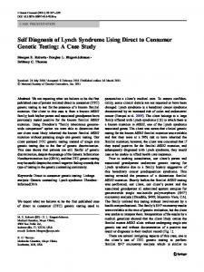
To illustrate the size of underestimation of both primal and dual TFP in the presence of imperfect competition and non-constant returns to scale, we plot the average growth rate of industry primal and dual TFP and the estimated primal and dual productivity growth in Figure 4. The growth rates of the estimated industry productivity are constructed using the consistent estimates on industry markup and returns to scale according to Column (7) of Table 3. The first observation from Figure 4 is that the difference between industry primal and dual TFP growth rate is almost negligible, which is evident from our Proposition 3, since factor shares have been relatively constant. Moreover, controlling for imperfect competition and non-constant returns to scale, the estimated growth rates of primal and dual productivity are consistently higher than the growth rates of primal and dual TFP. The differences are most prominent for industries that have high capital input growth such as the electronics industry. The simple average of the annual growth rate of productivity of all the industries from 1974 to 1992 is more than 7%, whereas the corresponding simple average of the growth rates of industry TFP is less than 3%. In other words, by correcting for imperfect competition and non-constant returns to scale, the underlying true productivity growth of the industries in the Singapore manufacturing sector is shown to be more than double what could be measured by the conventional growth accounting techniques.
20
6.
Robustness Checks
6.1
Real Value Added as Real Output
There may be a concern about the data because the growth rate of real value added was used instead of the growth rate of real output in the regression. As pointed out in Basu and Fernald (1995, 1997), because of the construction of the value added statistics, the growth rate of real value added will not be independent of the growth rate of intermediate input if the market is not perfectly competitive, even if the production function is weakly separable. Thus, using growth rate of real value added as the dependent variable may omit an important variable.9 In order to control for this omitted variable problem, the growth rate of nominal intermediate input is included in the regression. For reasons of data availability, the growth rate of nominal intermediate input is included in the regression instead of the growth rate of real intermediate input and the growth rate of relative prices, which are suggested by the theory (see Appendix). Thus, we are implicitly imposing the assumption that both regressors have the same coefficient. But since prices of intermediate input are not easily available, growth rate of nominal intermediate input is the second best alternative. The results are reported in Table 5. We perform a likelihood ratio test to verify the explanatory power of the growth rate of intermediate input in the regression. We are happy to find that even though the growth rate of intermediate input as a whole has significant explanatory power according to the test, the point estimates of industry markups and returns to scale are not statistically different from those listed in Table 2. In fact, only two industries have an even lower estimate of the returns to scale coefficients when the growth rate of intermediate input is included. This could be because growth rates of labor-capital ratio and capital input are not statistically correlated with the growth rate of intermediate input in the data. 9
For a detailed exposition of the claim, please refer to the Appendix.
21
6.2
Efficiency Labor Input
Data on the growth rate of labor input are constructed from the growth rate of number of workers in the industry. Thus, implicitly, the assumption of homogeneous labor input is imposed. But it is reasonable to believe that one unit of labor input in the 1990s should have higher productivity than one unit of labor input in the 1970s due to the accumulation of human capital of the economy. The homogeneous labor input assumption may bias the estimated coefficient due to the problem of error in measurement. More specifically, let Lit denote unit of physical labor and Leit denote unit of efficient labor, Leit = eit Lit ,
(32)
where eit indicates the level of efficiency of labor input in industry i in period t. We can modify our production function to incorporate labor efficiency: Yit = Ait F (Leit , Kit ) .
(33)
Thus Equation (9) can be adjusted to ˆ eit + αiK K ˆ it Yˆit = Aˆit + αiL L ³ ´ ˆ it + eˆit + αiK K ˆ it = Aˆit + αiL L
(34)
ˆ it . Yˆit = Aˆit + αiL eˆit + αiL ˆlit + Si K
(36)
(35)
or
Hence, there may be an omitted variable problem in our regression due to the mismeasurement of labor input. The resulting estimates of the regression may be biased. However, if the increase in human capital is homogeneous across industries, then the effect of eˆit will be captured in our period-specific effect, λt . Similarly, if the increase in efficiency is industry specific, then omitting eˆit will not be problematic as it will be explained by the industry-specific effect, ai . 22
Thus, the inclusions of period-specific effect and industry-specific effect will reduce the potential bias of the estimates due to the mismeasurement of labor input.
6.3
Capacity Utilization of Capital Input
In the regression, the growth rate of the service of capital input is proxied by the growth rate of capital input of the industries. In other words, full capacity utilization of capital input is assumed in the model. However, it is well known in the literature that the capacity utilization of capital input may fluctuate over the business cycle. Thus, without adjustment on the rate of utilization of capital input, there may be an error in variable problem in the regression. To illustrate this point, let Kit be the physical capital input and σit be the rate of utilization of the capital input. Thus, the service of the capital input is Kits = σ it Kit .
(37)
The production function can again be modified: Yit = Ait F (Lit , Kits ) .
(38)
Thus, Equation (9) can be adjusted to ˆ it + αiK K ˆ its Yˆit = Aˆit + αiL L ³ ´ ˆ it + σ ˆ it + αiK K = Aˆit + αiL L ˆ it
(39)
ˆ it , Yˆit = Aˆit + αiK σ ˆ it + αiLˆlit + Si K
(41)
(40)
or
´ ³ ˆ it > 0 due to business cycle fluctuation. with cov Aˆit , σ
Hence, without adjusting for capacity utilization, we again introduce an omitted variable
problem in the regression, which may result in bias in estimation of the regression.
23
One way to correct for the variability of the utilization of capital input is to use an instrument to proxy its rate. Harrison (1994) uses a measure of total energy used as the instrument. However, not all capital is electrical machinery and not all electricity consumption is due to the use of capital. The inclusion of total energy used in the regression may in turn introduce some extra noise into the estimation. Fortunately, the inclusion of the period-specific effect, λt , takes care of the business cycle fluctuation that is common across industries. Shocks that are specific to an industry will be captured by the industry-specific dummies. Thus, without introducing any extra variable, we are able to control for the capacity utilization of capital input.
7.
Conclusion
The dual equivalence of Hall’s (1988) technique is derived and tested. This paper shows that, theoretically, the presence of either imperfect competition or decreasing returns to scale technology will cause both primal and dual TFP growth rates to underestimate actual productivity growth. The size of bias depends on the degree of deviation from perfect competition and constant returns to scale. On the other hand, the difference between the growth rates of primal and dual TFP depends on the change in factor shares in revenue. Given that, in general, factor shares are relatively constant, the difference between the two TFP measures is close to zero, even if imperfect competition or non-constant returns to scale exist. These are the main theoretical findings of the paper, and it can be viewed as a complement to Hall (1988, 1990) and a contradiction to the results of Roeger (1995). The empirical section of this paper focuses on establishing a procedure that is capable of estimating actual productivity growth, even in the presence of imperfection competition and non-constant returns to scale technology. A panel regression that embraces both the primal and dual approaches is proposed to fully utilize information derived from both the quantity 24
and price sides of the data. We also present an empirical model that follows an Olley and Pakes (1996) type correction for input endogeneity and selection bias at an industry level to estimate the average industry markup and returns to scale. Using Singapore’s manufacturing sector as a case study, the empirical result of this paper shows that both the primal and dual regressions are empirically equivalent. In addition, all industries in the sector violated at least one of the assumptions of perfect competition and constant returns to scale. Controlling for input endogeneity and selection bias, the estimated average annual growth rate of productivity of the sector is more than 7%, which far exceeds both conventional measures. Thus, the regression result casts doubt on Young’s (1992, 1995) findings, as it suggests that the productivity growth of Singapore may be much higher than what can be measured using the conventional growth accounting technique. In other words, without testing the two assumptions of perfect competition and constant returns to scale, one should exercise caution when using conventional TFP measures.
25
A
Homogeneity of the Cost Function
Proposition 5 (A1) Let C (w, r, F (L, K)) = wL + rK, and Y = AF (L, K) . If F is homogeneous of degree S in (L, K) ,then 1. C is homogeneous of degree 2. C is homogeneous of degree 3. Let m =
∂C ∂Y ,
then m =
1 S 1 S
in F in Y
1C SY.
Proof. 1
1. Increase both L and K by δ S times, δ > 0 : ´´ ³ ³ 1 1 = C (w, r, δF (L, K)) , by homogeneity of F (L, K) . C w, r, F δ S L, δ S K Since C is homogeneous of degree 1 in (L, K) , the left-hand side of the above equation 1
1
can be reduced to δ S C (w, p, F (L, K)) . Thus, C (w, p, δF (L, K)) = δ S C (w, p, F (L, K)) implies that C (w, p, F (L, K)) is homogeneous of degree
1 S
in F (L, K) .
2. Notice that Y is homogeneous of degree 1 in F. Thus, C is homogeneous of degree F ⇒ C is homogeneous of degree
1 S
B
= S1 C ⇒ m =
in
in Y.
3. By Euler equation of homogeneous function, C is homogeneous of degree ∂C ∂Y Y
1 S
1 S
in Y ⇒
1C SY.
Input Elasticity, Revenue Share, and Cost Share
Definition 6 Let αX = θX = cX =
∂F X , the elasticity of output with respect to input X; ∂X F wX , the payment share of input X in total revenue; pY wX , the payment share of input X in total cost. C
Proposition 7 (A2) Let Y = AF (L, K) be the production function of a firm, and F be homogeneous of degree S in L and K. Let µ be the price over marginal cost markup. Let firm minimize cost. Then 26
1. αX = µθ X , X = L, K 2. cX = S1 αX = Sµ θX , X = L, K 3. cL + cK = 1 4. αL + αK = S 5. θL + θK = Sµ . Proof. 1. Firm facing given w and r, minimize the following program: min C = wL + rK s.t. Y
= AF (L, K)
⇒ L = wL + rK − λ (AF (L, K) − Y ) F.O.C.: w = λA By Envelope Theorem, m =
∂C ∂Y
∂F ∂L
= λ, the marginal cost of production. Thus,
w wL ∂F = ⇒ αL = = µθL . mA ∂L mY Similarly, αK = µθK . 2. By Proposition (A1), m =
1C SY
cL =
⇒ C = SmY. Thus, wL 1 wL 1 = = αL = µθL . C SmY S S
Similarly, cK = S1 αK = S1 µθK. 3. cL + cK =
wL C
4. αL + αK =
+
rK C
= 1, by the definition of C.
∂F L ∂L F
+
∂F K ∂K F
= S, by Euler equation for homogenous function.
5. θL + θK = cL Sµ + cK Sµ , by 2. ⇒ θL + θK = (cL + cK ) Sµ = Sµ , by 3.
27
C
Real Value Added vs. Real Output
To understand this problem, we need to go back to the construction of the real value added statistics. According to the Report on the Census of Industrial Production of Singapore, the nominal value added statistic is generated by subtracting the cost of intermediate input, including materials, utilities, and operating cost, from the value of output. Formally, let vt denote the real value added in period t, pt Yt be the value of output, and pMt Mt be the cost of intermediate input. Then the nominal value added is defined as pt vt = pt Yt − pMt Mt .
(42)
To find the growth rate of real value added, differentiate Equation (42) with respect to time: ∂vt ∂pt ∂Yt ∂pMt ∂Mt ∂pt vt + pt = Yt + pt − Mt − pMt . ∂t ∂t ∂t ∂t ∂t ∂t
(43)
Using the notation of growth rate, we can simplify Equation (43) to ˆ t. pt vt pˆt + pt vt vˆt = pt Yt pˆt + pt Yt Yˆt − pMt Mt pˆMt − pMt Mt M Let sM =
pMt Mt pt Yt ,
(44)
the share of intermediate input in total output. Dividing both sides of
Equation (44) by pt Yt and rearranging the terms, we can get ³ ´ ˆ t − pˆt (1 − sM )ˆ vt = Yˆt − sM pˆMt + M or 1 sM ˆ sM vˆt = Yˆt − Mt − 1 − sM 1 − sM 1 − sM
µd¶ pMt . pt
(45)
Thus, the growth rate of real value added is a weighted average of the growth rate of output and intermediate input (deflated by price of output). To link this with our earlier regression, we need to define a production function that
28
includes intermediate input. Let Yt = At F (Lt , Kt , Mt ) ˆ t + αK K ˆ t + αM M ˆ t, Yˆt = Aˆt + αL L where αM =
∂F M ∂M F ,
(46)
the elasticity of intermediate input with respect to output.
Substituting Equation (46) into Equation (45) , we will get 1 αL ˆ αK ˆ αM − sM ˆ sM Aˆt + Lt + Kt + Mt − vˆt = 1 − sM 1 − sM 1 − sM 1 − sM 1 − sM
µd¶ pMt . pt
Recall that αM = µsM , and αL +αK = S, the degree of returns to scale, and 1−sM =
(47) pt v t pt Yt .
Equation (47) can be simplified further to vˆt = =
µd¶ µ wpttYLtt 1 S s s pMt M M ˆ t + (µ − 1) ˆt − Aˆt + pt vt ˆlt + K M 1 − sM 1 − sM 1 − sM 1 − sM pt pt Yt µd¶ 1 S s s pMt M M ˆ t + (µ − 1) ˆt − Aˆt + µθLˆlt + K M . (48) 1 − sM 1 − sM 1 − sM 1 − sM pt
So when we regress the growth rate of real value added, vˆt , on the growth rate of labor per capital weighted by the share of labor in value added, θLˆlt , and the growth rate of capital, ˆ t , in order to estimate the markup coefficient, µ, and the scale coefficient, S, we need to K worry about a few things. First, the growth rate of intermediate input must be included together with the growth ´ ³ pMt ˆ t and d rate of relative prices in order to avoid the problem of omitted variables. If M pt
ˆt are omitted, then the estimated mark-up and scale coefficient will be biased, since ˆlt and K ³d´ . are correlated with Mt and ppMt t ³d´ Second, even if both Mt and ppMt are included in the regression, the estimated scale t
coefficient, S, as well as Aˆt , will be overestimated, as 1 − sM is less than one. In the data,
the size of sM ranges from 40% to 90%. Thus, we need to take this into account when we interpret the regression.
29
REFERENCES Aw, Bee Yan, Xiaomin Chen, and Mark J. Roberts (2001). “Firm-Level Evidence on Productivity Differentials and Turnover in Taiwanese Manufacturing,” Journal of Development Economics, vol. 66, no. 1, p. 51-86. Bartelsman, Eric J., Ricardo J. Caballero, and Richard K. Lyons (1994). “Customerand Supplier-Driven Externalities.” The American Economic Review, vol. 84, no. 4, p. 1075-1084. Basu, Susanto, and John G. Fernald (1995). “Are Apparent Productive Spillovers a Figment of Specification Error?” NBER Working Paper No. 5073. Basu, Susanto, and John G. Fernald (1997). “Returns to Scale in US Production: Estimates and Implications.” Journal of Political Economy, vol. 105, no. 2, p. 249-283. Caballero, Ricardo J., and Richard K. Lyons (1990). “Internal Versus External Economies in European Industry.” European Economic Review, vol. 34, p. 805-830. Caballero, Ricardo J., and Richard K. Lyons (1992). “External effects in U.S. Procyclical Productivity.” Journal of Monetary Economics, vol. 29, p. 209-225. Christensen, Laurits R., and Dale W. Jorgenson (1969). “The Measure of U.S. Real Capital Input, 1919-67.” Review of Income and Wealth, series 15, no. 4, p. 293-320. Hall, Robert E. (1988). “The Relation between Price and Marginal cost in U.S. Industry.” Journal of Political Economy, vol. 96, no. 5, p. 921-947. Hall, Robert E. (1990). “Invariance Properties of Solow’s Productivity Residual.” Growth / Productivity / Unemployment, ed. Peter Diamond, MIT Press, p. 71-112. Harper, Michael, Ernst R. Berndt, and David O. Wood (1989). “Rates of Return and Capital Aggregation Using Alternative Rental Prices.” Technology and Capital Formation, ed. Dale W. Jorgenson and Ralph Landau, MIT Press, p. 331-372. Harrison, Ann E. (1994). “Productivity, Imperfect Competition and Trade Reform: Theory and Evidence.” Journal of International Economics, vol. 36, p. 53-73. Hsieh, Chang-Tai (1998). “What Explains the Industrial Revolution in East Asia? Evidence from Factor Markets.” Princeton University Discussion Papers in Economics #196, Woodrow Wilson School of Public and International Affairs. Hsieh, Chang-Tai (1999). “Productivity Growth and Factor Prices in East Asia.” The American Economic Review, vol. 89, no. 2, p. 133-138. Jorgenson, Dale W., F. M. Gollop, and B. M. Fraumeni (1987). Productivity and U.S. Economic Growth. Amsterdam: North-Holland. Jorgenson, Dale W., and Martin A. Sullivan (1981). “Inflation and Corporate Capital Recovery.” Depreciation, Inflation and the Taxation of Income from Capital, ed. Charles R. Hulten, p. 171-237. Krugman, Paul (1994). “The Myth of Asia’s Miracle.” Foreign Affairs, vol. 73, no. 6, p. 62-78. Levinsohn, James (1993). “Testing the Imports-as-Market-Discipline Hypothesis.” Journal of International Economics, vol. 35, p. 1-22. 30
Levinsohn, James, and Amil Petrin (1999). “When Industries Become More Productive, Do Firms? Investigating Productivity Dynamics.” NBER Working Paper, no. 6893. Levinsohn, James, and Amil Petrin (2000). “Estimating Production Functions Using Inputs to Control for Unobservables.” NBER Working Paper, no. 7819. Olley, G. Steven, and Ariel Pakes (1996). “The Dynamics of Productivity in the Telecommunications Equipment Industry.” Econometrica, vol. 64, no. 6, p. 1263-1297. Roberts, Mark J., and James R. Tybout (1996). Industrial Evolution in Developing Countries: Micro Patterns of Turnover, Productivity, and Market Structure, Oxford: Oxford University Press. Roberts, Mark J., and James R. Tybout (1997). “The Decision to Export in Colombia: An Empirical Model of Entry with Sunk Costs.” American Economic Review, vol. 87, p. 545-564. Roeger, Werner (1995). “Can Imperfect Competition Explain the Difference between Primal and Dual Productivity Measures? Estimates for U.S. Manufacturing.” Journal of Political Economy, vol. 103, no. 2, p. 316-330. Wong, Fot-Chyi, and Wee-Beng Gan (1994). “Total Factor Productivity Growth in the Singapore Manufacturing Industries During the 1980’s.” Journal of Asian Economics, vol. 5, no. 2, p. 177-196. Young, Alywn (1992). “A Tale of Two Cities: Factor Accumulation and Technical Change in Hong Kong and Singapore.” NBER Macroeconomics Annual 1992. p. 13-53. Young, Alwyn (1995). “The Tyranny of Numbers: Confronting the Statistical Realities of the East Asian Growth Experience.” Quarterly Journal of Economics, vol. 110, no. 3, p. 641-668.
31
Table 1: Data at a Glance, 1974-1992
SSIC Industry Name 311/312 Food 313 Beverage 314 Tobacco 321 Textiles 322 Apparel 323 Leather 324 Footwear 331 Wood 332 Furniture 341 Paper 342 Printing 351 Industrial Chemicals 352 Chemical Products 353/354 Petroleum 355 Natural Rubber 356 Rubber Products 357 Plastic Products 361/362 Glass 363 Clay 364 Cement 365 Concrete Products 369 Mineral Products 371 Basic Metal 372 Non-Ferrous Metal 381 Fabricated Metal 382 Machinery 383 Electrical 384 Electronics 385 Transport Equipment 386 Scientific Instruments 390 Other 300 Industry Average
Output Capital Ratio -0.070 -10.564 -9.956 0.496 1.615 -4.187 -6.344 -1.512 0.088 -0.841 -0.951 1.015 0.311 0.245 2.796 -0.325 0.806 -4.702 -4.265 2.807 -1.126 -4.200 -4.502 5.330 -0.873 1.322 1.704 1.805 3.100 4.750 -4.832 -1.002
Real Rental Price -1.239 -9.149 -9.824 1.190 1.680 -5.891 -3.992 -1.855 0.750 -1.037 -1.146 0.879 0.696 -0.202 1.937 -1.573 0.063 -2.709 -3.363 2.678 -1.152 -5.769 -5.692 4.906 -1.089 0.020 1.686 1.982 2.985 4.809 -5.572 -1.129
Average Annual Growth Rates of Labor Rental Revenue Capital Wage Capital Rental 1 1 Ratio Ratio Input Ratio -2.458 -3.190 8.235 8.965 -4.345 -3.034 15.304 13.889 -3.605 -3.483 12.049 11.918 -4.168 -3.525 0.211 -0.483 -3.502 -3.435 6.770 6.704 -5.960 -7.660 11.429 13.132 -8.314 -5.972 7.383 5.031 -4.618 -4.963 -0.169 0.174 -3.381 -2.720 10.699 10.037 -3.831 -4.028 12.218 12.414 -3.485 -3.681 11.973 12.168 -1.695 -1.828 13.326 13.462 -1.726 -1.339 12.127 11.742 -0.168 -0.634 2.871 3.319 -2.527 -3.395 -1.797 -0.939 -2.362 -3.612 5.666 6.914 -2.269 -3.017 12.209 12.953 -6.935 -4.881 14.155 12.162 -5.505 -4.637 7.467 6.565 -0.930 -1.112 4.899 5.029 -2.834 -2.878 14.505 14.531 -2.778 -4.341 7.266 8.834 -2.004 -3.228 7.117 8.307 -0.496 -0.973 3.288 3.711 -2.968 -3.184 12.930 13.147 -2.554 -3.873 10.426 11.727 -4.024 -4.038 9.958 9.976 -3.067 -2.886 16.888 16.710 -2.801 -2.908 7.290 7.406 -1.876 -1.038 3.453 3.273 -4.982 -5.721 13.211 13.952 -3.296 -3.394 8.818 8.927
Primal 2 TFP 2.388 -6.219 -6.351 4.665 5.117 1.773 1.969 3.105 3.469 2.991 2.535 2.710 2.036 0.413 5.323 2.038 3.075 2.233 1.240 3.737 1.708 -1.422 -2.498 5.825 2.095 3.876 5.728 4.872 5.902 6.626 0.150 2.294
Dual Real 3 TFP Investment 1.951 9.434 -6.115 5.421 -6.341 8.127 4.715 -10.219 5.115 -2.808 1.769 13.029 1.980 -2.413 3.108 -9.001 3.470 8.772 2.991 10.523 2.534 10.682 2.707 8.436 2.035 9.963 0.432 11.574 5.332 -3.469 2.040 6.556 3.080 8.388 2.172 17.494 1.274 -3.408 3.790 0.577 1.726 17.745 -1.427 -4.684 -2.464 2.217 5.880 14.306 2.094 9.806 3.893 7.105 5.724 6.827 4.868 14.543 5.893 3.228 5.847 1.460 0.149 6.206 2.265 5.691
Average Firms' Turnover 4 Rate 101.553 99.172 95.725 99.974 102.707 99.326 99.220 96.051 105.952 102.096 103.676 108.026 101.197 103.222 96.230 99.798 106.002 101.502 97.185 103.426 103.769 101.898 100.197 107.849 105.384 106.164 103.546 108.995 104.171 104.267 102.788 102.293
Notes: Unless otherwise stated, all values represent the average annual growth rates from 1974 to 1992 in percentage terms. 1. Variable is multiplied by the share of labor in total revenue according to the specification of the model. 2. The growth rate of primal TFP is obtained by subtracting the growth rate of output-capital ratio from the growth rate of labor-capital ratio. 3. The gowth rate of dual TFP is obtained by subtracting the growth rate of real rental price from the growth rate of rental-wage ratio. 4. Firms' turnover rate is defined as the ratio of the number of firms across two consecutive years.
32
Table 2: Dependent Variables — Growth Rates of Real Output and Rental Price Method: Fixed Effect Panel Regression Included observations: 36 Included cross sections: 31 Total panel (unbalanced) observations: 1115 Robust Estimated S.E. Industry Markups Food Beverage Tobacco Textiles Apparel Leather Footwear Wood Furniture Paper Printing Industrial Chemicals Chemical Products Petroleum Natural Rubber Rubber Products Plastic Products Glass Clay Cement Concrete Products Mineral Products Basic Metal Non-Ferrous Metal Fabricated Metal Machinery Electrical Electronics Transport Equipment Scientific Instruments Other R-squared Adjusted R-squared S.E. of regression Log likelihood Durbin-Watson stat
1.70** 1.09* -0.01 1.50*** 1.78*** 1.21*** 1.23*** 0.90*** 1.15*** 1.26* 1.55*** 3.75*** 4.57*** 5.92*** 0.86*** 1.37*** 1.91*** 1.68*** 2.03*** 3.43*** 2.98*** 1.12*** -0.79 1.85*** 1.58*** 2.97*** 1.12*** 2.16*** 1.5*** 1.11 1.64*** 0.782142 0.758514 0.119426 845.2303 1.843607
Estimated Scale Robust Coefficients S.E.
(0.73) 0.62 (0.63) 0.15 (0.79) -0.52* (0.18) 0.64*** (0.21) 1.25*** (0.21) 0.51*** (0.28) 0.74*** (0.26) 0.33 (0.15) 0.79*** (0.60) 0.59** (0.32) 1.00*** (0.54) 1.31*** (1.40) 1.10** (1.30) 0.2 (0.27) -0.05 (0.20) 0.55** (0.17) 0.81*** (0.11) 1.13*** (0.25) 0.98*** (0.6) 0.01 (0.23) 0.96*** (0.19) 0.4** (1.03) -1.47*** (0.21) 0.77** (0.27) 0.98*** (0.23) 1.47*** (0.17) 0.40** (0.23) 0.73*** (0.29) 0.63*** (0.74) 0.23 (0.21) 0.74*** Mean dependent var S.D. dependent var Sum squared resid F-statistic Prob(F-statistic)
Notes: *, **, and *** indicate significance at 90%, 95%, and 99% confidence levels, respectively. Industry and year fixed effects are included but not reported.
33
(0.53) (0.22) (0.31) (0.19) (0.23) (0.16) (0.25) (0.27) (0.07) (0.34) (0.22) (0.31) (0.51) (0.49) (0.21) (0.16) (0.17) (0.09) (0.14) (0.28) (0.10) (0.16) (0.56) (0.34) (0.21) (0.18) (0.20) (0.19) (0.19) (0.51) (0.19) -0.01 0.243 14.334 46.258 0
Table 3: Olley-Pakes Correction (1) Dependent Variable
Estimated industry markup Estimated industry scale coefficient
(2) (3) Growth Rate of Output per Capital
1.52*** (0.08) 0.62*** (0.10)
Investment growth
1.47*** (0.08) 0.64*** (0.10) 0.03*** (0.01)
Polynomial of investment and capital stock growth Powers of the estimated lagged productivity growth Powers of the estimated lagged survival probability Polynomial of estimated lagged productivity and survival rate Year fixed effects Industry fixed effects Sample size
(4) Firms' Turover Rate
1.44*** (0.09)
(5)
(6) (7) Growth Rate of Output per Capital - 1.44*Growth Rate of Labor per Capital 1.44*** 1.44*** 1.44*** (0.09) (0.09) (0.09) 0.60*** 0.58*** 0.57*** (0.03) (0.08) (0.08)
3rd order 4th order 3rd order 3rd order 3rd order
Yes Yes 1115
Yes Yes 1115
Yes Yes 1115
Yes Yes 1115
Yes Yes 1083
Yes Yes 1083
Yes Yes 1083
Notes: Robust standard errors in parentheses. *, **, and *** indicate significance at 90%, 95%, and 99% confidence levels, respectively. Estimated productivity growth is obtained from the fitted value of the polynomial of investment and capital growth from Column (3). Estimated survival rate is the fitted value of Column (4).
34
0
-5
-10 Food Beverage Tobacco Textiles Apparel Leather Footwear Wood Furniture Paper Printing Industrial Chemicals Chemical Products Petroleum Natural Rubber Rubber Products Plastic Products Glass Clay Cement Concrete Products Mineral Products Basic Metal Non-Ferrous Metal Fabricated Metal Machinery Electrical Electronics Transport Equipment Scientific Other
Table 4: TFP vs. Estimated Productivity Growth
15
10
5
%
Primal T FP Growth Dual T FP Growth
Estimated Primal Productivity Growth Estimated Dual Productivity Growth
35
Table 5: Dependent Variables: Growth Rates of Real Output and Rental Price (controlling for the growth rate of intermediate input cost) Method: Fixed Effect Panel Regression Included observations: 36 Included cross sections: 31 Total panel (unbalanced) observations: 1115 Robust Estimated S.E. Industry Markups Food Beverage Tobacco Textiles Apparel Leather Footwear Wood Furniture Paper Printing Industrial Chemicals Chemical Products Petroleum Natural Rubber Rubber Products Plastic Products Glass Clay Cement Concrete Products Mineral Products Basic Metal Non-Ferrous Metal Fabricated Metal Machinery Electrical Electronics Transport Equipment Scientific Instruments Other R-squared Adjusted R-squared S.E. of regression Log likelihood Durbin-Watson stat
2.09*** 0.96 -0.17 0.23 1.49*** 0.69** 1.10*** 0.86 0.45** 0.4 1.50*** 3.42*** 5.15*** 7.24*** 0.86*** 0.81** 1.01** 1.91*** 1.18*** 2.30*** 2.12*** 1.00*** -0.5 1.82*** 1.10** 2.04*** 0.76*** 1.50*** 1.21*** 0.86 1.03*** 0.812598 0.785661 0.112513 929.1809 1.901742
Estimated Scale Robust Coefficients S.E.
(0.84) 0.84 (0.64) 0.15 (0.82) -0.59 (0.26) 0 (0.25) 1.17*** (0.29) 0.18 (0.27) 0.71*** (0.65) 0.33 (0.19) 0.36*** (0.77) 0.24 (0.32) 1.01** (0.51) 1.2*** (1.10) 1.08*** (1.37) 0.74*** (0.25) -0.03 (0.39) 0.35* (0.50) 0.37 (0.21) 1.24*** (0.31) 0.57*** (0.74) -0.04 (0.37) 0.72*** (0.17) 0.28*** (1.05) -1.38** (0.24) 0.71*** (0.53) 0.73*** (0.36) 1.21*** (0.22) 0.28 (0.50) 0.48* (0.42) 0.48** (0.92) 0.01 (0.30) 0.38* Mean dependent var S.D. dependent var Sum squared resid F-statistic Prob(F-statistic)
(0.66) (0.25) (0.31) (0.17) (0.27) (0.20) (0.24) (0.54) (0.11) (0.40) (0.21) (0.33) (0.43) (0.35) (0.20) (0.18) (0.33) (0.12) (0.16) (0.27) (0.11) (0.13) (0.57) (0.31) (0.33) (0.22) (0.22) (0.28) (0.22) (0.69) (0.22) -0.010013 0.243026 12.33006 38.74653 0.000000
Notes: *, **, and *** indicate significance at 90%, 95%, and 99% confidence levels, respectively. Industry and year fixed effects are included but not reported. Growth rate of intermediate input is included but not reported.
36