1
13/12/13
Current understanding of the processes underlying the triggering of and energy loss associated with type I ELMs A. Kirk1, D. Dunai2 M. Dunne3 G. Huijsmans4, S. Pamela1, M. Becoulet5, J.R. Harrison1, J. Hillesheim1, C. Roach1, S. Saarelma1 1
EURATOM/CCFE Fusion Association, Culham Science Centre, Abingdon, Oxon, OX14 3DB, UK KFKI RMKI, Association EURATOM, Budapest, Hungary 3 Max-Planck Institut für Plasmaphysik, EURATOM Association, Garching, Germany 4 ITER Organization, Cadarache, St. Paul-lez-Durance, France 5 Association Euratom/CEA, CEA Cadarache, F-13108, St. Paul-lez-Durance, France 2
Abstract
The type I ELMy H-mode is the baseline operating scenario for ITER. While it is known that the type I ELM ultimately results from the peeling-ballooning instability, there is growing experimental evidence that a mode grows up before the ELM crash that may modify the edge plasma, which then leads to the ELM event due to the peeling-ballooning mode. The triggered mode results in the release of a large number of particles and energy from the core plasma but the precise mechanism by which these losses occur is still not fully understood and hence makes predictions for future devices uncertain. Our current understanding of the processes that trigger type I ELMs and the size of the resultant energy loss are reviewed and compared to experimental data and ideas for further development are discussed.
2
1.
Introduction The type I ELMy H-mode is the baseline operating scenario for ITER [1]. Extrapolations for the amount of energy released by Type I Edge Localised Modes (ELMs) in ITER, based on data from existing tokamaks, indicate that the largest ELMs could not be tolerated regularly because of the damage they would cause [2] and so finding a way of reducing the energy released is essential [3]. However, there is considerable uncertainty associated with such predictions because of the lack of understanding of all of the processes involved. The type I ELM is thought to result from the peeling-ballooning MHD instability [4]. In this theory the edge pressure gradient grows in the inter-ELM period until the
peeling-ballooning stability boundary is crossed at which point the ELM is triggered. However, as will be discussed in this paper it has been observed on several devices that the experimental profiles can exist near to this stability point for a substantial amount of the inter-ELM period raising the question: what ultimately triggers the ELM? While the particle and energy losses from the plasma due to a type I ELM have been measured on a range of devices, including detailed measurements of the changes to the plasma profiles over the ELM crash, there is no detailed quantitative understanding of how these losses occur. In this paper the current status of experimental measurements will be compared with results from models to review the current understanding of the processes that determine when a type I ELM is triggered and the resulting energy losses that occur. The layout of the paper is as follows: Section 2 describes the evolution of the edge plasma profiles during the
3
inter-ELM period and examines the detailed changes that occur just before a type I ELM is triggered. In particular, it examines new evidence for a pre-cursor mode, attempts to identify it and discusses the role it may play in the ELM crash. Section 3 reviews the experimental evidence related to energy losses associated with type I ELMs and compares these observations with toy models and state of the art non-linear codes. Section 4 summarises the findings and discusses the direction for future studies. 2.
What triggers a type I ELM? 2.1 Type I ELM cycle
There are two basic ideal MHD instabilities associated with ELMs: the ballooning mode and the peeling mode [5]. The peeling mode is associated with the edge current density, while the ballooning mode is driven by the pressure gradient. The often referred to picture for the evolution of the edge profiles between type I ELMs is that the pressure gradient increases on the transport time scales until it reaches the ballooning instability boundary, where further evolution of the gradient is clamped by high n (where n is the toroidal mode number) ballooning modes. The edge current then rises on resistive time scales, which were assumed to be slower, until the peeling-ballooning stability boundary is reached at which point a medium n instability is generated, the type I ELM. This leads to the loss of energy and particles which reduce the edge pressure and current until stability is reached. However, recent calculations have suggested that the edge pressure and current profiles evolve on very similar timescales during the inter-ELM cycle i.e. the edge pressure gradient is not established significantly in advance of the edge current.
4
Direct measurement of the edge current profile are still in their infancy [6][7]. On DIII-D the current profile during the inter-ELM period has been extracted using conditional averaging for multiple ELMs and does suggest some small but finite lag between the evolution of the pressure gradient and the edge current density [8].
Calculations of the
current diffusion performed for ASDEX Upgrade discharges, show that the edge current density evolves on the same time scale as the temperature and density gradients [9][10]. The edge current density has also been reconstructed from magnetic measurements on ASDEX Upgrade using the CLISTE equilibrium code [11]. The evolution of the peak edge current density determined by this method versus the local peak edge pressure gradient is shown in Figure 1.
An almost linear trend between the two quantities is observed
throughout the ELM cycle and hence there is no evidence for a resistive delay in the buildup of the edge current density [12]. Similar results have been observed on DIII-D [13] where in this case the edge current density is calculated using the Sauter formula (see figure 8 in reference [14]). In all of these cases the edge current and pedestal pressure gradient evolves to the peeling-ballooning stability boundary before the ELM is triggered but the ELM is not always triggered immediately when the stability boundary is reached/crossed.
For
example, on ASDEX Upgrade in some discharges the ELM is triggered immediately in others the profiles stop evolving and the pressure gradient remains stationary for a considerable fraction (up to 50 %) of the inter-ELM period before the ELM [10]. The local maximum pressure gradient being constant does not imply the distance to the stability limit is the same. In fact, on MAST it has been observed that although the pressure gradient remains fixed during most of the ELM cycle, the pressure pedestal height and width
5
continue to growing [15]. The increasing width then reduces the stability limit such that it comes down to the experimental point shortly before the ELM. In addition there are uncertainties in both the modelling and the experimental measurements but there is increasing evidence that the pedestal profiles exist in or near to the unstable region for a time before the ELM is triggered. This is particularly noticeable on JET, in a high refuelling scenario, where the pedestal profiles are stationary, near to the peeling-ballooning boundary, for 60 % of the ELM cycle [16]. This suggests that there must be some process that is stabilising the peeling-ballooning mode and, as will be discussed in the next section, one possibility for this is the edge velocity shear.
2.2 Growth of the peeling-ballooning mode
The Wilson and Cowley model [17] of the ELM predicts the explosive growth of the mode. The mode structure is elongated along a field line, localised in the flux surface, perpendicular to the field line and relatively extended radially. The ballooning mode grows explosively as the time approaches a “detonation” time when the theory predicts the explosive growth radially of narrow filaments of plasma, which push out from the core plasma into the Scrape Off Layer (SOL). Such filament structures have been observed experimentally, initially, using visible imaging on MAST [18] and subsequently using a variety of diagnostics on a range of devices (see [19] and references therein).
The
observation of filaments alone is not a proof of this model, however, because ballooning modes can also give rise to filaments. To prove the explosive part it would be necessary to show that the mode grows faster than exponential. At present there is no experimental evidence for or against an explosive growth and this should be the subject of future work.
6
An example of the observation of the toroidal/poloidal motion of the filament once they are beyond the LCFS is shown in Figure 2, which shows a wide angle view of ASDEX Upgrade plasma. Figure 2b shows an image obtained just after the start of the rise of the target Dα light associated with an ELM. Clear stripes are observed, which are on the outboard (low field side) edge of the plasma. In order to make the filaments more visible and to aid in analysis, a background subtraction is performed, which produces the image shown in Figure 2c. Figure 2d and e show the original and background subtracted images obtained 50 µs (5 frames) later where the filaments have rotated toroidally/poloidally in the co-current direction (or poloidally downwards in the ion diamagnetic direction) and 3 of the filaments have interacted with the ICRH limiter. The interactions show up as bright spots in the image. The toroidal mode number of these filaments is typically in the range 12-18. In the Wilson Cowley model these filaments grow by twisting to push through magnetic field lines without reconnection and so would be impeded by the velocity shear that is known to exist in the pedestal region of the plasma (see for example [20][21]). Stability calculations have also suggested that the growth rate of the peeling-ballooning modes may be sensitive to the velocity and/or velocity shear in the pedestal region [22]. In fact in the presence of such a shear, it is difficult to see how the filament could squeeze between the field lines on neighbouring flux tubes i.e. they would most likely get distorted or even may be broken off as a blob of plasma. The evolution of the toroidal rotation of the bulk plasma during an ELM has been measured at the edge of the plasma on DIII-D [20] and MAST [21]. Before the ELM there is a steep velocity gradient at the edge of the plasma. As the ELM progresses this shear is
7
at first reduced and then removed completely before quickly recovering after the peak in Dα emission (see figure 1 in [20] and figure 13 in [21]). The start of the change in velocity occurs effectively at the same time as the Dα light starts to rise. There is little evidence that the change in velocity precedes the ELM, however, it should be noted that the integration time of these diagnostics are ~ 200 µs. Hence changes on time or spatial scales less than the resolution of the diagnostics may have been missed. Although when the filaments have pushed out beyond the LCFS they clearly rotate in the co-current direction, there is the possibility that as the filaments push through the LCFS their poloidal rotation is small. Figure 3 shows measurements of the plasma edge during the ELM crash using a turbulence imaging beam emission spectroscopy (BES) diagnostic on MAST [23] which images a 8x16 cm region at the edge of the plasma with a 2cm spatial and 500 kHz temporal resolution. The first frame (t0) shows the formation of the filament inside the LCFS. In the next 10 µs the filament extends out radially and then moves downwards poloidally in the co-current direction. In the next subsection how these filaments propagate though a region of high velocity shear will be discussed and in particular if there is any evidence for pre-cursor activity that could modify the edge plasma.
2.3 Evidence for pre-cursor activity
Evidence for pre-cursors with a high toroidal mode number that grow up before the crash of a type I ELM has been obtained in a variety of diagnostics on several devices. Fluctuations have been observed using ECE measurements on ASDEX Upgrade [24] and reflectometry on JT-60U [25]. These fluctuations are observed to grow up ~200 µs before the ELM and
8
to be localised in a narrow region near to the top of the pedestal. On MAST density fluctuations have been observed in line average density measurements in the 100 µs before the filaments due to the ELM become visible at the Last Closed Flux Surface (LCFS) [26]. Pre-cursors have also been observed in magnetic sensors on JET [27] and in the coupling of ICRH into the plasma on both JET and AUG [28], which indicated that the perturbation rotated in the counter current (or electron diamagnetic) direction, although it was not clear if this rotation was for the pre-cursor of for the entire ELM event. Recently 2D ECE imaging performed on KSTAR [29] and ASDEX Upgrade [30] has measured the rotation of the pre-cursor activity. A pre-cursor mode is observed to grow ~ 200 µs before an ELM is triggered rotating in the electron diamagnetic (counter current) direction. The mode has a poloidal wavelength of 15 cm and radial size of 3cm, rotating with an apparent poloidal velocity of ~5 kms-1 in the electron diamagnetic direction. The fluctuation frequency is ~20-50 kHz. On MAST, a mode with similar characteristic has also been observed using the BES system [31].
Figure 4
shows the 2D images of the normalised density fluctuations
separated in time by 5 µs. A clear upwards propagation of a mode structure can be observed. This upwards motion corresponds to a rotation in the counter current or electron diamagnetic direction. The mode is observed to start to grow about 100 µs before the ELM crash, with a frequency of ~20 kHz. It is located radially near to the top of the pedestal. The mode has a poloidal wavelength of ~ 10cm and a radial size of ~2cm. The toroidal mode number, n ~30-40. At the onset of the mode it is observed to rotate in the counter current direction while the background turbulence is observed to rotate in the co-current
9
direction. The mode is observed to grow in size until it appears to lock the entire flow in the pedestal region (i.e. bring it to zero), at which point the filament structures associated with the ELM are observed to grow [31].
This mode has also been identified on MAST
using Mirnov coils located on the low field side of the plasma [31] and using the Doppler back scattering (DBS) diagnostic. There is evidence that this mode may actually exist for a large proportion of the inter-ELM period but it fluctuates in size, remaining quite small until becoming strong ~ 100 µs before the ELM crash. Gas puff imaging has been used to capture the two-dimensional evolution of type I ELM pre-cursors on NSTX [32]. This again shows that strong edge intensity modulations propagate in the electron diamagnetic direction while steadily drifting radially outwards. The intensity fluctuations were observed at frequencies around 20 kHz and wavenumbers of 0.05–0.2 cm−1. Once in the SOL, the filaments reverse their propagation direction and travel in the ion diamagnetic direction. Edge intensity fluctuations are strongly correlated with magnetic signals from Mirnov coils. In summary, recent observations on a wide variety of devices suggest that an electromagnetic pre-cursor mode located near to the pedestal top with a high toroidal mode number propagates in the electron diamagnetic direction and grows up rapidly just before a type I ELM crash. In the next subsection the possible identification of this mode will be discussed. 2.4 Identification of the pre-cursor mode
Recently there has been significant effort in performing gyro-kinetic simulations of the pedestal region. These studies have been motivated by an attempt to understand the
10
microinstabilities that may ultimately determine the properties of the pedestal and in particular the pedestal width. The EPED model [33] proposes that drift wave turbulence is suppressed in the pedestal region by sheared flow and that turbulence associated with the kinetic ballooning mode (KBM) then constrains the pedestal to a critical normalized pressure gradient. The gyrokinetic code, GS2 [34], has been used for microstability analysis of the edge plasma region in MAST [15], JET [16] and NSTX [35]. In these simulations, while KBMs sometimes show up in the steep gradient pedestal region, Microtearing mode (MTM) are always found in the plateau region near to the top of the pedestal [36][37]. The MTM is an electromagnetic mode that is fundamentally driven by the electron temperature gradient and exists when the plasma normalised pressure (β) exceeds a critical value. The mode rotates in the electron diamagnetic direction, is stabilized by the density gradient and has a broadband frequency spectrum with poloidal wavenumber 0.6∆Ti. However, this is not observed experimentally where ∆Te~∆Ti [48]. As will be discussed later this may be too simplified a conclusion and in order to make quantitative predictions for ELM energy losses, models need to capture all the processes. In the remainder of this section the key elements that may lead to ELM energy losses will be investigated, at first using toy models to discuss the role of filaments and edge ergodisation before looking at how the state of the art models correctly incorporate both effects into describing the entire ELM loss process. 3.1 The role of filaments in the energy loss process
Filament structures have been observed during ELMs on a number of devices [19] and these filaments have been shown to lead to the spiral patterns observed on the divertor [49][50]. Direct measurements have been made on MAST [50] and JET [51] and other devices of the energy content of the filaments. The maximum energy content of a single filament (assuming Ti=Te), observed close to the LCFS on both devices, is ~2.5 % of ∆WELM, but this may well be an under estimate since in the SOL Ti>Te [52].
The
observations would suggest that the maximum amount of ELM energy transported by the separated filaments would be 25 % of ∆WELM (Ti = Te) or 50 % of ∆WELM (Ti = 3Te) for 10 equally sized filaments. Note that this assumes all the filaments have the maximum size observed and hence is likely an over estimate. Taking into account the spread in the measured energy content of the filaments and assuming that Ti=Tiped (the ion temperature at
15
the pedestal top), the total amount of energy carried away by the separated filaments is ~ 25-30% of ∆WELM, which is in good agreement with the amount of ELM energy arriving at the first wall [53]. This means that 70-75 % of the ELM energy has to be lost, either by the filaments while they remain attached to surface inside the LCFS or by another process. Filaments exist near the LCFS for 50 -100 µs at the start of the ELM event and are born as elongated field aligned structures, which have an initial parallel extent covering the low field side of the plasma. The rise time of the divertor ELM energy flux is correlated with the ion parallel transport time (τ// = L///cs, where L// is the parallel connection length from the mid-plane to the divertor and cs is the ion sound speed) [54], and a detailed analysis of the temporal evolution of the ELM power target deposition in AUG and JET reveals that the ELM energy must be released from the core in ≤ 80 µs [55].
The
correlation between this loss time and the time over which the filaments exist to the LCFS has led to the development of “leaky hosepipe” ELM energy loss models [56][50] where the filaments act as conduit for particles and energy from the confined plasma to the divertor. These models assume that the filament structures are linked to the core for a time duration of τELM. During this time the filament acts as a conduit for losses from the pedestal region into the SOL either by convective parallel transport due to a reconnection process (where one end of the filament remains attached to the core while other end becomes connected into the SOL) or by increasing the cross-field transport into the SOL. According to the predictions of non-linear ballooning mode theory, close to marginal stability τELM~(τΑ2τΕ)1/3, where τA is the Alfvén time and τE is the energy confinement time [57]. The total number of particles that could flow down n filaments is given
16
by N fil = nΓσ filτ ELM , where Γ is the average particle flux density ( Γ =
1 1 8kT ), nc = n 4 4 πmd
ere md is the mass of deuterium) and σ fil is the cross sectional area of the filament. The average particle flux density is calculated using the pedestal density and temperature respectively.
The energy lost due to an ELM would then be given by the parallel
convective heat equation i.e. ∆WELM = 52 k (Ti ped + Te ped ) N fil . Assuming the filaments have a circular cross section, and using the measured widths, the ELM energy losses obtained from the model (assuming Ti ped = Te ped ) compared to the measured energy losses on MAST and JET are shown in Figure 5. The ELM energy loss model predictions are in reasonable agreement with the data given the crude nature of the model. However, what is not described is how the energy actually gets out of these filaments. Does one end of the filament reconnect into the LCFS while the other remains attached to the core, or does the perturbation to the field lines caused by the filaments increase cross field transport? Until the actual loss mechanism is established these models cannot be used to reliably extrapolate to future devices.
3.2The role of ergodisation
In order to explain the ELM energy loss mechanism models based on the ergodisation of the edge plasma have been proposed where the ergodisation is driven by currents in the SOL or the filaments. As will be discussed in the next sub-section, the ergodisation does not need to be produced by current carrying filaments since it can be produced by the magnetic fluctuations associated with the ballooning mode itself. In the case of current
17
carrying filaments, these currents are either thermoelectric in nature localised by intrinsic error fields [58][59] or due to the dynamo effect [60]. These models find that the plasma edge can be ergodised, and manifold structures form, when localised currents of 200-300 A are present. These values for the current are very similar to those observed experimentally in ELM filaments [61][62][63].
Models where the ELM energy loss is through
ergodisation by current carrying filaments are attractive because they not only allow a mechanism by which the energy and particles can be removed from the core but also allow a mechanism for turning off the loss process as can be demonstrated with a toy model. Consider starting off with 12 current carrying filaments located on the q95=5 surface on MAST, where each filament carries 200 A (see Figure 6a). The effect that these filaments have on the edge plasma can be calculated, in the vacuum approximation using the ERGOS code [64], which is usually used to calculate the effect that externally applied resonant magnetic perturbations (RMPs) have on the plasma.
In the case of current
carrying filaments they are generated along field lines and hence the magnetic perturbations they produce are perfectly aligned with the equilibrium field. They therefore easily create island structures that overlap in the edge of the plasma (see Figure 7). In MAST experiments with externally applied RMPs there is a threshold in the normalised radial resonant field component (brres) of the applied RMP field of brres ~ 0.5x10⁻³, below which the applied RMPs have little effect on the plasma [65]. As can be seen in Figure 8 when the filaments are at the q95 surface the peak value of brres = 4x10⁻³ so a large effect would be expected on the plasma edge may be expected. As the filaments separate and move away from the LCFS (Figure 6b and c) the maximum value of brres decreases rapidly and by the time the filament is 5cm from the
18
LCFS the value of brres has approached the threshold value and hence the loss processes could be assumed to have stopped. These calculations have been done in the vacuum approximation and it is likely that if plasma screening is included the field would falloff much more quickly as the filaments move away from the LCFS. ELM energy loss through ergodisation has certain implications that can be tested either now or in future experiments. Firstly, the splitting of the divertor strike point is a common observation in the presence of external non-axisymmetric magnetic perturbations (see for example [66][67][68][69]).
Therefore edge ergodisation may be expected to
produce a splitting of the strike point while the filaments are still inside the LCFS, and this splitting will be in addition to that produced once the filaments have separated. With ever faster cameras becoming available this is something that could be investigated in future experiments. Secondly the ergodisation would affect both the high and low field sides of the plasma and hence enhanced losses would occur to both the inner and outer divertor. However, in connected double null plasmas effectively no ELM energy goes to the high field side target (see for example [70][71][72]). But this may just point to our lack of understanding of how transport occurs in ergodic fields. For example, according to the Rechester–Rosenbluth model electron transport should dominate in the presence of an ergodic field and hence it may be expected that the dominant change would be to the electron temperature pedestal with little change to the ion temperature, which is not observed.
The main consequence of applying RMPs to H-mode plasmas at low
collisionality is the so called “density pump out” effect where the pedestal density drops while the temperature pedestal remains unaltered (see [73] and reference therein). In the case of RMPs this observation can be explained by changes in the radial electric field
19
[74][75][76][77]. In particular it is found that due kinetic effects [77], the stochastic parallel thermal transport is significantly reduced compared to the prediction from the standard Rechester–Rosenbluth model [78]. The parallel electron heat transport is found to be approximately the same as the particle transport, which is significantly enhanced due to the changes in the radial electric field (Er). The inclusion of such effects in modelling of the ELM should be a subject of future work.
3.3State of the art modelling
Several non-linear codes have been developed in recent years to study the crash phase of ELMs. Considerable progress has been made and the codes are approaching realistic resistivities and are starting to see experimental phenomena and trends. Whilst some qualitative agreement has been achieved, the ability to accurately predict ELM sizes from first principles has not yet been demonstrated. Several nonlinear simulation codes have been applied to ELM simulations, including BOUT [79], BOUT++[80][81], GEM [82][83], JOREK [38][84][85], NIMROD [86][87] and M3D [88]. These employ different physical models, as well as a range of numerical methods. An unresolved issue is which set of equations is most relevant to ELM simulations, and what difference this makes to the predictions. M3D [88], JOREK [38], BOUT++ and gyrofluid modelling [83] have reported ergodisation of the edge due to the magnetic fluctuations associated with the ballooning mode. For example, non-linear simulations of ELMs using the JOREK code [89] indicate that the footprint for the energy deposition pattern on the divertor is influenced by the
20
ejection of filaments (which depends on their radial velocity) and heat conduction along homoclinic tangles (which depends on the size of magnetic perturbation) [90]. The lobe structures resulting from homoclinic tangles produced by the application of RMPs have been observed experimentally [91][92] . The challenge will be to see if similar structures can be observed during ELMs and disentangled from the effect that the filaments have in the X-point region. These non-linear simulations have now reached a stage where they can be compared in detail with experimental data (see for example [84][85]). The simulated filament size and energy content are similar to the experimental observed ones [85] but the filaments are often more regularly spaced than in the experiment possibly due to the fact the simulations are often performed with only a single mode number. They are able to reproduce many of the divertor target foot print features and match well the experimentally observed broadening of the strike point with increasing ELM size [89]. However, to date they have not been able to match the in/out target heat load asymmetries observed on, for example, JET and ASDEX Upgrade [89]. In order to simulate the energy loss the codes often include a parallel conduction model (see for example [84]). While the incorporation of this enables the experimentally observed ELM energy loss scaling with collisionality to be recovered it does mean that the codes predict a larger change in the electron temperature compared to the ion temperature.
Figure 9 shows the fractional change in the electron
and ion temperature profiles from before to after the ELM crash for the discharge modelled in reference [84].
Unlike the experimental observation, the change in the electron
temperature profile is more than twice the change in ion temperature. This could be due to the choice of sheath boundary conditions chosen for this simulation. However, it should
21
be noted that the change in ion temperature is not negligible because some of the changes in the ion temperature result from the expansion of the filaments into the SOL. 6-field simulations carried out with BOUT++ have shown cases where the ELM energy loss is mainly via the ion channel [93] but these simulations are for plasmas with a circular crosssection and it is not clear if they correctly capture the parallel loss processes. In all these cases the non-linear simulations of ELMs start from an MHD unstable state i.e. the pedestal profiles have to be increased beyond the peeling-ballooning stability limit. The ELM size depends on the initial linear growth rate and hence how far above stability the simulation is started and this makes it difficult for them to reliably predict the ELM amplitude. 4. Summary and discussion In the inter-ELM stage of a type I ELM-ing discharge the pedestal pressure and current evolve on the transport time scale towards the peeling-ballooning stability limit. At some point the edge parameters cross this MHD stability boundary, the location of which can be reliably calculated using linear MHD codes. While ultimately it is the peeling-ballooning mode that leads to the type I ELM crash, the edge parameters can exist near to this unstable region for a substantial part of the inter-ELM period. There is growing experimental evidence that another mode grows up at the pedestal top that rotates in the electron diamagnetic direction and possibly reduces the edge flow shear sufficiently to allow the peeling-ballooning mode to grow explosively. Hence it would be appear that the flow shear at the pedestal top may be important for suppressing type I ELMs. In fact, exactly
22
such a mechanism has been suggested as the reason that type I ELMs are suppressed in the QH-mode [94][95]. At least two types of pre-cursor have been observed one at high toroidal mode number (n~30-40) and one at low (n~1-2). In contrast to the peeling-ballooning mode which have intermediate toroidal mode numbers of n~10-15. The exact nature of the precursor mode and the mechanism that triggers it is unclear, it could possibly be associated with micro tearing modes or else it could be a linear state of the peeling (for the low n) or ballooning (high n) modes. Ballooning mode simulations at very high Reynolds numbers (S=2x10⁸) have shown the presence of pre-cursors before the ELM onset. The pre-cursor perturbation is located mostly inside separatrix and produces oscillation of ballooning mode at mid-plane, however, at present these simulations show that the toroidal mode number of the pre-cursor and peeling-ballooning mode are the same. Filaments resulting from the peeling-ballooning mode clearly play some part in the ELM energy loss mechanism and it is likely that edge ergodisation also plays a role. At present the experimental measurements for this ergodisation are inconclusive. The nonlinear models have now advanced to such a stage that they can now reproduce a lot of the experimentally observed phenomena. For example, they observe the formation of the filaments and the structure in the divertor heat flux profiles. But they have little predictive capability on the ELM amplitude. This is because most non-linear MHD simulations start from an MHD unstable state and the ELM size depends on the initial linear growth rate, which in terms depends on the distance above marginality. The inclusion of stabilisation by flows (diamagnetic, toroidal, poloidal) and how the loss of stabilisation occurs in the non-linear phase including the braking of flows due to MHD may be important to make
23
progress in this area. It should be noted that the explosive growth of the ELM, which allows fast growth even close to marginal stability has yet to be observed in non-linear MHD simulations but as discussed earlier neither has it been observed experimentally. If the trigger for the ELM crash can be determined, the next question is what are the loss mechanisms and what determines the final post ELM pedestal state, which is well below the marginal stability limit? At present the models suggest two loss processes one based on the filaments and the other based on ergodisation. Filaments arise due to the formation of ballooning interchange convective cells which move across the separatrix. There is parallel convective and conductive transport to divertor while the filament moves towards the wall.
The magnetic perturbations due to the ballooning mode create
homoclinic magnetic tangles, which give a direct connection from inside the pedestal to the divertor and parallel conductive losses occur with a strong temperature dependence. However, these loss mechanisms still do not capture the observed changes in the ion and electron temperature profiles and it may be necessary to include kinetic effects in the model. This may be possible by coupling the MHD codes with kinetic codes as was reported in the coupling of the XGC0 code with M3D [96].
Acknowledgement This work was part-funded by the RCUK Energy Programme [grant number EP/I501045] and the European Communities under the contract of Association between EURATOM and CCFE. To obtain further information on the data and models underlying this paper please contact
[email protected]. The views and opinions expressed herein do not necessarily reflect those of the European Commission
24
References [1] ITER Physics Expert Group 1999 Nucl. Fusion 39 2391 [2] Loarte A et al. 2002 Plasma Phys. Control. Fusion 44 1815 [3] Lang P T et al 2013 Nucl. Fusion 53 043004 [4] Connor J W 1998 Plasma Phys. Control. Fusion 40 531 [5] Wilson HR et al., 2006 Phys. Control. Fusion 48 A71
[6] Thomas D et al. 2004 Phys. Rev. Lett. 93 064003 [7] de Bock M et al., 2012 Plasma Phys. Control. Fusion 54 025001 [8] Thomas D et al., “Edge current growth and saturation during the type I ELM cycle”
33rd EPS Conference on Plasma Phys. Rome, 19 - 23 June 2006 ECA Vol.30I, P-5.139 (2006) [9] Wolfrum E et al., 2009 Plasma Phys. Control. Fusion 51 124057 [10] Burckhart A et al., 2010 Plasma Phys. Control. Fusion 52 105010 [11] Mc Carthy PJ and ASDEX Upgrade Team 2012 Plasma Phys. Control. Fusion 54
015010 [12] Dunne M et al., “Edge current density behaviour during Type-I ELM cycles and ELM-
mitigation scenarios on ASDEX Upgrade” 2013 P5-05 Presented at 14th International Workshop on H-mode Physics and Transport Barriers Oct. 2-4, 2013 Kyushu University, Fukuoka, Japan [13] Groebner RJ et al 2010 Nucl. Fusion 50 064002
[14] Sauter O, Angioni C and Lin-Liu YR, 1999 Physics of Plasmas 6 2834 [15] Dickinson D et al., 2011 Plasma Phys. Control. Fusion 53 115010 [16] Saarelma S et al, 2013 Nucl. Fusion 53 123012 [17] Wilson H R and Cowley S C 2004 Phys. Rev. Lett. 92 175006 [18] Kirk A et al., 2004 Phys. Rev. Lett. 92 245002 [19] Kirk A et al., 2009 Journal of Nuclear Materials 390–391 727 [20] Wade M et al., 2005 Phys. Rev. Lett. 94 225001
25
[21] Kirk A et al., 2005 Plasma Phys. Control. Fusion 47 315 [22] Saarelma S et al., 2007 Plasma Phys. Control. Fusion 49 31 [23] Field AR et al., 2012 Rev Sci Instrum 83 013508 [24] Suttrop W et al,, 1996 Plasma Phys. Control. Fusion 38 1407 [25] Oyama N et al, 2004 Nucl. Fusion 44 582
[26] Scannell R et al, 2007 Plasma Phys. Control. Fusion 49 1431 [27] Perez CP et al., 2004 Nucl. Fusion 44 609 [28] Bobkov V et al., 2004 "Studies of ELM Toroidal Asymmetry Using ICRF Antennas at JET and ASDEX Upgrade"in: Europhysics Conference Abstracts (CD-ROM, Proc. of the 31st EPS Conference on Plasma Physics, London, 2004) , Vol. 28G (2004), P-1.141 [29] Yun GS et al., 2011 Phys. Rev. Lett. 107 045004 [30] Boom JE et al., 2011 Nucl. Fusion 51 103039 [31] Dunai D et al., “Measurement of type I ELM pre-cursors in MAST using Beam emission spectroscopy” In preparation. [32] Sechrest Y et al., 2012 Nucl. Fusion 52 123009 [33] Snyder P B et al 2009 Nucl. Fusion 49 085035 [34] Kotschenreuther M, Rewoldt G, and Tang WM, 1995 Comput. Phys. Commun. 88 128 [35] Canik J et al, 24th IAEA FEC, EX/P7-16, 2012 [36] Dickinson D et al., 2012 Phys. Rev. Lett. 108 135002 [37] Dickinson D et al., 2013 Plasma Phys. Control. Fusion 55 074006 [38] Huysmans G et al., 2007 Nucl. Fusion 47 659 [39] Webster A.J., 2012 Nuc. Fusion, 52 114023 [40] Sommer F et al 2011 Plasma Phys. Control. Fusion 53 085012 [41] Wenninger R et al, 2012 Nucl. Fusion 52 114025 [42] Wenninger R et al, 2013 Nucl. Fusion 53 113004
26
[43] Krebs I et al., 2013 Phys. Plasmas 20 082506 [44] Loarte A et al., 2002 Plasma Phys. Control. Fusion 44 1815 [45] Leonard AW et al 2003 Journal of Nuclear Materials 313 768 [46] Loarte A et al 2004 Phys. Plasmas 12 2668 [47] Hayashi N et al 2011 Nucl. Fusion 51 073015 [48] Wade M et al.,2005 Phys. Plasma 12 056120 [49] Eich T et al 2003 Phys. Rev. Lett. 91 195003 [50] Kirk A et al., 2007 Plasma Phys. Control. Fusion 49 1259 [51] Beurskens MNA et al 2009 Nucl. Fusion 49 125006 [52] Kocan M et al., 2011 J. Nucl. Mater. 415 S1133 [53] Herrmann A et al. 2004 Plasma Phys. Control. Fusion 46 971 [54]
Eich T et al. 2005 J. Nucl. Mater. 337-339 669
[55] Eich T et al. 2007 “ ELM divertor heat load in forward and reversed field in ASDEX Upgrade” Proc. 34th EPS Conference on Plasma Phys. Warsaw, 2 - 6 July 2007 ECA Vol.31F, P-2.017 [56] Becoulet M et al., 2003 Plasma Phys. Control. Fusion 45 A93 [57]Cowley SC, Artun M, 1997 Phys. Rep. 283 185 [58] Evans T et al 2009 Journal of Nuclear Materials 390 789 [59] Rack M et al., 2012 Nucl. Fusion 52 074012 [60] Alladio F. et al., 2008 Plasma Phys. Control. Fusion 50 124019 [61] Kirk A et al., 2006 Plasma Phys. Control. Fusion 48 B433 [62] Migliucci P et al. 2010 Phys. Plasmas 17 072507 [63] Vianello N et al., 2011 Phys. Rev. Lett. 106 125002 [64] Nardon E et al., 2007 J. Nucl. Mater. 363-365 1071
27
[65] Kirk A et al. 2013 Nucl. Fusion 53 043007 [66] Schmitz O et al 2008 Plasma Phys. Control. Fusion 50 124029 [67] Jakubowski M W et al 2009 Nucl. Fusion 49 095013 [68] Jachmich S et al 2011 J. Nucl. Mater. 415 S894 [69] Nardon E et al 2011 J. Nucl. Mater. 415 S914 [70] Petrie TW et al., 2003 Nucl. Fusion 43 910 [71] Kirk A et al., 2004 Plasma Phys. Control. Fusion 46 551 [72] De Temmerman G et al., 2011 J. Nucl. Mater. 415 S383 [73] Kirk A et al., 2013 Plasma Phys. Control. Fusion 55 124003 [74] Tokar M. Z., et al., 2008 Phys. Plasmas 15 072515. [75] Yu Q and Gunter S 2009 Nucl. Fusion 49 062001 [76] Rozhansky V., et al., 2010 Nucl. Fusion 50 034005 [77] Park G, Chang CS, Joseph I and Moyer RA 2010 Phys. Plasmas 17 102503 [78] Rechester AB and Rosenbluth MN 1978 Phys Rev Lett 40 38 [79] Snyder PB et. al. 2005 Phys. Plasmas 12 056115 [80] Dudson BD et. al. 2009 Computer Physics Communications 180 1467 [81] Dudson B et al., 2011 Plasma Phys. Control. Fusion 53 054005 [82] Scott B 2010 Contrib.Plasma Phys. 50 228 [83] Peer J et al.. 2010 Plasma Phys. Control. Fusion 52 075006 [84] Pamela S et. al. 2010 Plasma Phys. Control. Fusion 52 075006 [85] Pamela S et. al. 2013 Plasma Phys. Control. Fusion 55 095001 [86] Pankin AY et al., 2007 Plasma Phys. Control. Fusion 49 S63 [87] Burke BJ et. al. 2010 Phys. Plasmas 17 032103
28
[88] Sugiyama LE et. al.2009 J. Phys. Conf. Ser. 180 012060 [89] Huijsmans G et al., 2013 J. Nucl. Mater. 438 S57 [90] Huijsmans G et al.,2013 Nucl. Fusion 53 123023 [91] Kirk A et al., 2012 Phys. Rev. Lett. 108 255003 [92] Schaffer MJ et al. 2012 Nucl. Fusion 52 122001 [93] Xia T et al., 2013 Nucl. Fusion 53 073009 [94]Oyama N et al.,2006 Plasma Phys. Control. Fusion 48 A171–A181 [95] Burrell K et al., 2009 Nucl. Fusion 49 085024 [96] Park G et al., .2007 J. Phys. Conf. Ser. 78 012087
29
Figures
Figure 1 The peak edge current (jpeak) vs the radial pressure gradient (dP/dr) calculated using the CLISTE equilibrium code as a function of time during an inter-ELM period on ASDEX Upgrade.
30
Figure 2 Visible images obtained on ASDEX Upgrade. a) full view of the plasma with the region of fast acquisition shown as a box. b) image obtained during the start of the rise time of the target Dα due to an ELM and d) an image obtained 50 µs later during the same ELM. c) and e) are background subtracted versions of b and d respectively.
31
Figure 3 Turbulence imaging of the plasma edge during an ELM crash on MAST using a Beam Emission Spectroscopy system. The frames shown are separated in time by 5µs relative to a notional crash time (t0). The dotted curve in the first frame shows the location of the last closed flux surface.
32
Figure 4 Turbulence imaging of the plasma edge during the pre-cursor stage leading up to a type I ELM crash on MAST using a Beam Emission Spectroscopy system. The frames shown are separated in time by 5µs relative to a notional time (t0), which is ~100 µs before the ELM crash. The dotted curve in the first frame shows the location of the last closed flux surface.
33
Figure 5 Measured ELM energy loss (∆WELMexp) versus the ELM energy loss calculated using a “leaky hosepipe” model (∆WELMmodel) for a) MAST and b) JET.
Figure 6 Simulation of 12 equal toroidally spaced current carrying filaments located a) inside the LCFS on the q95=5 surface, b) 1cm and c) 10 cm outside the LCFS for a MAST like plasma in a connected double null magnetic configuration.
34
Figure 7 Calculated island size (squares) and distance between islands (crosses) calculated in the vacuum approximation assuming 12 equally space filaments, each carrying 200 A, located at the q95=5 surface.
Figure 8 Radial profile of the normalised resonant component of the applied field (brres) for 12 equally space filaments each carrying 200 A located inside the LCFS at the q95=5 surface (crosses) and a distance of 1 (circles) 5 (squares) and 10 cm (diamonds) outside the LCFS.
35
Figure 9 JOREK simulations of the changes in the electron (solid) and ion temperature profiles due to an ELM in JET normalised to the temperature before the ELM.