by the I-beam post anchor and guy cables, provided central ... welded at equally spaced angles to a 0.55 m (1.8 ft) length .... 0 to 5 L min-1 (0 to 1.3 gal min-1 ). ..... 16.O0bcd. 17.10bccl. 15.85cd. 17.70d. 9.00e. 11.03f. 25-50. 1. 27.90. 31.30.
MASTER COPY MEASURING WIND AND LOW-RELIEF TOPOGRAPHIC EFFECTS ON RAINFALL DISTRIBUTION R. D. Lentz, R. H. Dowdy, R. H. Rust Advances in agricultural technology are giving farmers the capability to selectively manage soils of smaller and smaller areal dimension, and the capacity to alter management practices on the go. Farmers need to better understand the nature of within-field variability if they are to adjust their management accordingly. We hypothesized that wind interacts with low-relief topographic features and significantly alters rainfall distribution in the landscape. To determine wind and topographic effects on rainfall distribution across agricultural landscapes, rainfall intensity measurements have typically been made in situ. Problems associated with this method involve finding appropriate field sites, observational uncertainties, and logistical complications. For a study of rain on low hills, we avoided such problems by using a full-sized replica of a hill. Design and construction of this hill model are described. The apparatus emulated the slope and summit components of a low hill, and summit elevation was adjustable [1 to 3 m (3 to 10 ft)]. It was equipped with wind speed and direction sensors, and tipping-bucket flow-gages that measured natural precipitation intercepted by catchments located on windward and leeward slope positions. It automatically maintained a windward orientation during precipitation events, thus increasing the number of relevant measurements obtained in a given season. Results, obtained over two field seasons, indicate that hydrological rainfall varied significantly across different portions of the hill model. On average, hill positions experiencing maximum intensity received 1.5x more rain than those positions with the least precipitation. The rainfall pattern differed, depending on meteorological rainfall (intensity measured on level ground beyond the hill model), incident wind speed, and hill-summit elevation. This study shows that rainfall can vary across landscapes that include low-relief topographic features. The amount of variation is large enough to influence crop or plant growth, and other soil processes. Keywords. Agriculture, Automation, Landscape, Rainfall, Rainfall intensity, Spatial patterns,Topography, Water distribution, Wind. ABSTRACT.
ost research examining wind and topographic influences on rainfall distribution have relied on measurements taken on the particular M landscape feature of interest. Landforms involved in these studies varied in scale and shape, and included entire mountain ranges (Shermerhorn, 1967; Smallshaw, 1953), mountain ridge crests (Hovind, 1965), hill-bounded plains (Sandsborg, 1969), and ridge-shaped hills (Sharon, 1980; Jones et al., 1975). Relief ranged from 40 to several 1000 m. Relief in agricultural landscapes is often less than 5 m (16 ft). Few studies have determined how small topographic features influence rainfall distribution in farm fields, in spite of potential impacts that nonuniform rainfall has on crop productivity, erosion processes, and leaching regimes. Investigators encounter many difficulties when conducting landscape-based rainfall research. Problems include: 1) locating landforms with required shape and Article was submitted for publication in April 1994; reviewed and approved for publication by the Soil and Water Div. of ASAE in November 1995. Trade names and products are mentioned only for their informative value. No endorsement by the USDA-Agricultural Research Service or University of Minnesota is implied. The authors are Rodrick D. Lentz, Postdoctoral Fellow, Dept. of Agricultural Engineering, University of Idaho, Kimberly, Idaho; and Robert H. Dowdy, Soil Scientist, and Richard H. Rust, Professor, USDA-Agricultural Research Service and University of Minnesota, St. Paul.
fetch characteristics; 2) extended experimental periods needed to acquire adequate data on specific precipitation and wind events; 3) optimizing logistics involved in placement, installation, and maintenance of instrumentation, and travel to dispersed field sites; and 4) obtaining permission and cooperative agreements with land owners or operators. These complications can be avoided if a full-sized, appropriately instrumented model of the landform were constructed at an accessible field site. Further benefits accrue if the hill model is adjustable, permitting a change in conformation and relief, and orientation with respect to wind direction. When the apparatus is programmed to automatically orient itself into the prevailing wind, experimental observations can be obtained during any rainfall event, regardless of accompanying wind conditions. The objective of this study was twofold: 1) Design and construct an apparatus that would duplicate the shape of a low hill, permit adjustment of summit elevation [1 to 3 m (3 to 10 ft)], automatically orient its forward slope into the prevailing wind, and measure natural rainfall intercepted at different hill positions. 2) Test the hypothesis that rainfall across low hills is affected by incident wind. MATERIALS AND METHODS DESIGN AND CONSTRUCTION
Shape and relief of the hill model were selected to simulate small-scale topographic features that commonly
Applied Engineering in Agriculture VOL. 11(2):241-248
1995 American Society of Agricultural Engineers
t
'..;421.60n
241
LEEWARD SLOPE FRAME
.,/ ,
`,
C
SUMMIT SUPERSTRUCTURE . -1,-. . ---1--
1; / ./,// < < /6. `‘ \ ' .,: •:,\N
4b \ ',
WINDWARD SLOPE FRAME
WATERSHED POSITIONS
0 3b
,‘N. 0
WIND
0 Mgra
‘/‘,/, 3, a,/,,
„2
„;;>\ ) : 1
BA
,a.
B
SUMMIT CROSS FRAME
•
6. m
D I SUMMIT SUPERSTRUCTURE
PIVOT POST II SUMMIT FLOW GAUGE I I -SLOPE FRAME I I I
SLOPE FRAME
BASE FRAME 181111111llwilill 1 2 3 4 5 SCALE, METERS
GROUND LEVEL
STEEL RAIL POST ANCHOR
0
5 10 SCALE, FEET
15
Figure 1-Diagram of the hill model (drawn to scale): (A) side view showing all major frame components, (B) top view showing base frame and steel track, (C) top view of windward and leeward slope frames hinged to the summit superstructure, and (D) up-wind view detailing construction of the summit cross-frame.
242
APPLIED ENGINEERING IN AGRICULTURE
(A)
(B)
(C) Figure 2–Hill model: (A) installed at Rosemount Experiment Station, Minn., (B) view beneath covered slope frame showing runoff collection troughs, flow diverters, and tipping-bucket flow-gages, (C) motor and friction drive assembly that aligns hill model with prevailing winds.
occur in many cultivated areas in Minnesota. The apparatus was not intended to represent larger-scale geomorphic forms present in these landscapes. General Description. The hill model apparatus pictured in figures 1 and 2 reproduced the windward slope, summit, and leeward slope components of a hill. Six major units comprised the basic structure. The pivot post, held upright by the I-beam post anchor and guy cables, provided central
VOL. 11(2):241-248
support for the base frame; summit superstructure; and two slope frames (fig. 1A). A circular steel rail supported peripheral portions of the base and slope frames. The summit superstructure and slope frame were covered with polyethylene and sheet metal, this covering defined the hill's surface. The elevation of the summit superstructure was adjusted to modify hill model relief and sideslope angle. Post and Anchor. The post anchor was constructed of four steel I-beams [200 mm (8 in.)], each 1.5 m (5 ft) long, welded at equally spaced angles to a 0.55 m (1.8 ft) length of 6.4 mm (0.25 in.) thick steel pipe [I.D. 121 mm (4.75 in.)]. The anchor was buried in the earth. The 5.5-m (18-ft) pivot post, constructed from a 100 mm (4 in.) steel well casing, fit into the pipe sleeve and rotated freely on a steel ball bearing inserted between the post base and capped sleeve bottom. Base Frame and Summit. A rectangular frame [6 m x 13.7 m (20 ft x 45 ft)], constructed of 100-mm (4-in.) aluminum irrigation pipe, comprised the base frame of the hill (fig. 1B). It was aligned with the summit superstructure and fixed to the pivot post. The 3 m x 6 m (10 ft x 20 ft) summit superstructure (figs. 1A, C) was constructed of 22 mm (0.88 in.) square steel tubing. Convex summit frame members project in windward and leeward directions from a cross-frame backbone oriented perpendicular to the wind flow (fig. 1D). In profile (fig. 1A), the top surface of the hill summit forms a smooth arc 9.06 m (27.7ft) in radius. The crest rises 0.15 m (0.5 ft) above the summit's leeward and windward edges. The cross-frame was bolted to an upright steel pipe sleeve that fit over the pivot post. The superstructure was hoisted up the pivot post using a built-in winch and cable, and the summit sleeve was bolted to the post at selected elevations. Slope Frames. Two 6 m x 6 m (20 ft x 20 ft) slope frames constructed of 19-, 25-, and 38-mm (0.75-, 1.0-, and 1.5-in.) aluminum tubes were hinged to the windward and leeward edges of the summit (figs. 1A, C). The lower ends of the slope frames were attached with sliding mounts to the base frame, and were free to move horizontally when a summit height adjustment caused the slope frames to shift relative to the base frame. The superstructure, slope frames, and base frame were attached to and rotated in unison with the pivot post. The outermost portions of the base frame were supported by roller bearings that turned on a 13.9 m (45.5 ft) diameter circular steel track made from 6.4 x 76 mm (0.25 x 3 in.) flat steel, rolled to form an arc with 6.94 m (22.8 ft) radius. Rainfall Measurement. Aluminum sheet catchments at seven different positions on the summit and slopes of the hill model collected incident rainfall (fig. 1C). These large collecting surfaces(watersheds) were employed to avoid measurement errors associated with point-source sensors. Table 1 presents hill-model slope and watershed-position characteristics for different summit elevations. Runoff was measured with tipping bucket flow gages (fig. 2B). Eight flow gages were constructed using a modified version of the Biggerstaff and Moore (1984) design (Moore et al., 1983). A magnet attached to the tipping bucket momentarily closed a magnetic reed switch. The electrical pulses were counted using a Campbell Scientific CR-10 datalogger. Flow gages for summit catchments were
243
Table 1. General hill model, hill-component, and watershed characteristics for various model configurations General Hill Model Hill Configuration Relative Hill (Summit Elev.) Shape (H/L)• All 0.9m (3 ft) 1.8m (6 ft) 2.1m (7ft) 2.7m (9 ft)
n/a 0.21 0.43 0.50 0.65
Slope Component
Relative Watershed Positions - (100 x D)/1"t
Component Location
Slope (°)
Slope (%)
summit side-slope side-slope side-slope side-slope
62 6.0 15.4 18.4 24.1
13.8 13.3 34.2 40.8 53.5
0 n/a 94.00 94.04 94.06 94.11
1
2
n/a 64.04 64.27 6438 64.67
n/a 36.07 36.48 36.68 37.20
3 n/a 113 113 113 113
* H - elevation (m) of summit, L - horizontal distance (m) from the summit to a point on the slope with 0.5 x H elevation. f Position values for watersheds 4 to 6 are the same, but opposite in sign, as those for watersheds 1 to 3, respectively. D - horizontal distance (m) from watershed center to summit peak.
attached to a frame suspended from the superstructure's windward and leeward edges (fig. IA), and those for slope catchments were fixed to base-frame supports (fig. 2B). Flow Gage Calibration. Each gage (one per watershed) was calibrated with a constant head tank. The tank was connected via an adjustable orifice to an outlet tube, and supplied constant flow to the gage inlet. Flows ranged from 0 to 5 L min- 1 (0 to 1.3 gal min- 1 ). Each gage was tested at 6 to 10 flow rates,with 3 to 8 repetitions at each rate. Inflows were held constant prior to and during testing. A fifth-order polynomial function (eq. 1) was fitted to the calibration data and was employed to convert tip-rate (TP) in tips min- 1 to flowrate (FL), L min- 1 :
FL -E (c,x TP) i-
(1)
where Ci = coefficient of the polynomial calibration function exponential series for tip-rate TP; = degree of the polynomial function, plus one n (n = 6) Accuracy of calibration functions was evaluated by computing the 95% confidence error (0.5 x full confidence limit range) of the mean flowrate response at different tiprates. Since the confidence error varied depending on flowrate, it was reported as a weighted average. That is: 1) the flow range was divided into four subranges; 2) 95% confidence errors for flowrate observations were averaged within each flow subrange; and 3) an overall function mean was derived by averaging subrange values, weighted according to the proportion of the flow range included in each subrange. The error was given as a percent of the flowrate. Accuracy of flowrate, as predicted from tip-rate, was examined by computing the relative error. The above described weighted averaging procedure was employed here also, but the absolute values of the flowrate residuals were substituted for confidence error values. Relative error was reported as a percentage of the predicted flowrate. Meteorological Measurements. Meteorological rainfall intensity, as defined in the computations section, was measured over level terrain near the hill model, but beyond its zone of influence. A calibrated tipping-bucket rain gage (Texas Electronics, Inc., model 525), fitted with an expanded collecting surface to increase its sensitivity, was employed for this purpose. Incident wind speed and hill summit wind speed at 1 m (3.3 ft) height were measured with three-cup anemometers (Gill model 12102). Wind 244
direction was measured at the hill summit and on the lower leeward slope of the model with a wind vane (MET One model F1180). Wind vanes were installed so that their 180° azimuth was directed at the designated windward slope. Thus, deviation from 180° indicated that the hill model was misaligned with incident wind. Hill Model Operation. The model was erected in a level cropped area. No significant obstructions to wind flow were present within 150 m (500 ft) radius (10 hill model lengths) of the apparatus. The hill model was automated so that it was oriented into the wind continuously. A reversible gear motor, mounted on a corner of the base frame, supplied power to a friction drive in contact with the circular track (fig. 2C). The entire apparatus could be rotated by turning the friction wheel in the appropriate direction along the track circumference; maximum rotation rate was 13° min- I . The attached datalogger monitored wind speed and direction, controlled hill orientation, and recorded flow gage measurements (Lentz, 1991). The hill model was programmed to reorient itself with respect to the current wind direction every minute during rainfall events, every 15 min during dry periods when winds exceeded 2.5 m s- 1 (5.6 mile h- 1 ), and every 60 min under conditions of no rainfall and light winds (< 2.5 m s- 1 or 5.6 mile h- 1 ). The latter eliminated excessive motor operation when no rain data were being collected and wind directions were most variable (i.e., light winds). Current wind direction was computed as the 1-min mean during rain events and 15-min mean during dry intervals. The 1-min 'rain' orientation time was considered most practical, given the wind-azimuth shift-rates most prevalent during rain events. Shorter orientation times (< 1 min) were more likely to respond to short-term wind azimuth fluctuations and needlessly over work the drive mechanism. Data Output. Information stored by the datalogger varied depending on precipitation and wind conditions. During rainfall events, the time and identity of each bucket tip (pulse), total 1-min pulse count for each gage, and 1-min mean wind speed and direction for all sensors were recorded. During dry periods, only the 15-min mean wind speed and direction for all sensors were recorded. COMPUTATIONS
Rainfall Intensity Terms. Rainfall-intensity terms (Sharon, 1980) employed are defined below. Rainfall intensity is measured as depth per unit orifice area per unit time (mm h- 1 or in h- 1 ). Meteorological rainfall (MR) is intensity measured with a standard rain APPLIED ENGINEERING IN AGRICULTURE
gage having a horizontal orifice. This definition includes the assumption that MR is measured in a location that is level and free of local obstructions such as buildings, vegetation, and gross topographic features. MR=Rxcoscl)
(2)
where MR = given in mm h- 1 (in h- 1 ) R = rainfall intensity relative to a plane normal to rainfall vector (mm h- 1 ; in h- 1 ) = raindrop incidence angle in radians (positive to windward, vertical 0) Hydrological rainfall (HR) is that measured by a gage whose orifice is parallel to the surface slope; it corresponds to depth of rainfall actually intercepted by the surface. Computing HR. Datalogger records were downloaded as ASCII files onto a personal computer and reduced with an author written PASCAL program (HSMOUT61). The HSMOUT61 program provided output of 1-min records (the basic analytical unit) that included summit elevation, Julian day, ending time of the 1-minute averaging period, summit and incident wind speeds (m s- 1 ), misalignment ( 0 ) of hill model to windward, degree difference between summit and leeward wind azimuths, HR (mm h- 1 ) at each watershed position, MR (mm h- 1 ) away from the hill model, and a code indicating whether rain was increasing or decreasing. Data were considered valid if collected under the following conditions: 1) meteorological rainfall was at least 1 mm h- 1 (0.04 in h- 1 ); 2) all flow gages were recording flow during the period; this ensured that storage capacity of each watershed was filled, eliminating error caused by initial differences in catchment-to-flow-gage delivery rates between watersheds; 3) hill model was aligned properly to windward (geometric analysis indicated alignment should be within 10° of windward); 4) crop height in the surrounding field did not exceed 0.5 m (1.6 ft) during the data collection period. The HR was derived directly from watershed runoff measurements; values for duplicated catchments at summit positions were averaged. Mean tip-period values rather than tips-per-minute values were employed to calculate HR
Table 2. Calibration statistics for each watershed's tipping-bucket flow gage Standard Err. Est. (L min -1 )
Standard Err. Est. (gal min -1 )
95% Conf. Error* (%)
Relative Errort
(No.)
Calibration Function R2
24 41 55 55 43 42 43 53 38
0.999 0.998 0.998 1.000 0.998 1.000 0.999 0.997 0.998
0.0058 0.0742 0.0624 0.0281 0.0584 0.0239 0.0488 0.0792 0.0756
0.0015 0.0197 0.0165 0.0074 0.0155 0.0063 0.0129 0.0210 0,0200
5.54 3.91 3.78 1.66 3.65 2.10 2.45 4.14 6.04
2.42 1.88 1.65 0.84 2.41 1.00 2.41 2.80 2.15
Flow Gage
Samples
0 1 2 3a 3b 4a 4b 5 6
(%)
* Ninety-five percent confidence error surrounding mean flow rate at a given tips min -1 value, computed as a flow-rate weighted mean, and given as a percent of flow rate. t Relative error - Abs(Observed - Predicted)x (Observed)-1 x100, computed as a flow-rate weighted mean.
for each watershed; this permitted measurement of low intensity rainfall events. Hydrological rainfall (HR; mm h- 1 ; or with appropriate conversion constant, in h- 1 ) was computed by: HR=KxRxAw-1 (
3
)
where K = conversion constant FL = flowrate obtained from the flow gage calibration function (eq. 1), given TP as the reciprocal of the tip period (time between tips) Aw = watershed surface area (m2; ft2) RESULTS AND DISCUSSION
Polynomial functions were fit using least squares to 24 to 55 calibration data pairs obtained for each flow gage. Example calibration data and fitted function for flow gage no. 2 (for watershed 2) are presented in figure 3. Accuracy of flow rate measurements differed depending on flowrate, and relative errors ranged from 0.84 to 2.8% for the flow gages (table 2). This level of accuracy was better than that attained with other flow measuring devices (Barfield and Hirschi, 1986). The hill model was installed at Rosemount Experiment Station, Minnesota, in early spring of 1989. Testing revealed a need for only minor design modifications. Hill model alignment was successfully maintained except
Incident Wind Speed (mile h 30
0
5
10
15
20
1)
25
30
35
12
14
0.9 m (3 ft) Summit Elevation
20 10
-10 -20 .7• 2
Tips per Minute Figure 3-Example of calibration data for tipping-bucket flow-gage no. 2 (for watershed no. 2).
VOL. 11(2):241-248
4
6
8
10
Incident Wind Speed (m s 1 ) Figure 4-Wind azimuth deviations between 0.9 m (3 ft) hill model summit and leeward slope positions (when model was aligned within 10° of windward).
245
- 8
17 15 13
C Ty 7 § E6 250
• Watershed 3a
10
200
• Watershed
4a • Watershed 5
8
rc 150
- Incident Wind
4
50
2 79 81 83 85 87 89 91
0 1
E E .c
0 0
-10 lT
6
100 0 77
Distance (ft) C
20
40
60
80
Au
100
Wind •••••7411, 2.7 ms (6 mile 11-1 )
MR Vw 54.6 mm 11 1
0.4
0.0
C
-0.4 0 1 2 3 4 5 6 f Hill Profile
-20 ,'- (2.1 in h 1 )
Cc
-0.8
CC 0
5
15 20 25 30 35
10
Distance (m)
0 93
Time (min) Figure 5-Hydrologic rainfall received at selected watershed positions (fig. IC) during a precipitation event. Hill model elevation was 2.7 m (9 ft) and event winds averaged 6.6 m s- 1 (14.7 mile h- 1 ).
during the initial phase of many rainstorms, when associated gust fronts caused wind shifts of 45° to 90° in a period of 1 to 3 min. A plot of summit and leeward wind azimuth differences (fig. 4) provides an indication of the wind flow pattern across the hill model when the summit height was 0.9 m (3 ft). Deviations occurred within a narrow range (± 5°) for all the recorded incident wind speeds, except those below 1.5 m s- 1 (3.3 mile h- 1 ). This suggests that air flows linearly across the hill model when incident wind speeds exceeded 1.5 m s- 1 (3.3 mile h- 1 ). At lower velocities, airflow across the hill occasionally lacked the energy to ascend the summit; instead, the air at lower elevations became blocked and was forced to flow around the barrier (Baines, 1979). The flow path of converging air on the leeward hill slope differed significantly from that at the summit position, resulting in large summit-leeward wind azimuth deviations. Hence, hill model data collected at wind speeds below 1.5 m s- 1 (3.3 mile h- 1 ) may have been more variable because of the occasional occurrence of a blocked wind condition. An example of hill model intensities measured during a precipitation event is given in figure 5. Hill-model summit elevation was 2.7 m (9 ft) and incident wind speed during
Figure 6-Hydrologic rainfall occurring at watershed positions during a 1-min period, given as deviations from MR (MR HR on level surface beyond the hill model). Hill model elevation was 2.1 m (7 ft), 1-min mean wind speed was 2.7 m s- 1 (6 mile h-'), and meteorological rainfall (MR) was 54.6 mm h-' (2.1 in. h- 1 ).
the storm averaged 6.6 m 5- 1 (14.8 mile h- 1 ). Graphed points are rainfall values computed at each recorded tip (from tip period) and data were smoothed (averaged over 0.3-min periods) to eliminate short-term fluctuations. For simplicity, only three watershed locations (defined in fig. 1C) are shown. Relative HR differences between watersheds decrease as rainfall intensity declines. This may be related to a simultaneous decline in wind speed (14%) that occurs at minute 84; or it may simply reflect the shifting intensity distribution that occurs when the general rainfall rate declines from very high to low values. While these plots clearly showed rainfall differences between hill slope components, the format was not amenable to statistical analyses of several different incident-MR or wind speed classes. Another form of data presentation was required. A second approach utilized data averaged over 1-min periods. Distribution of hydrological rainfall across the hill model, when the summit was set to 2.1 m (7 ft) elevation, is presented in figure 6. The data represent a 1-min snapshot of HR across the hill when incident wind speed was 2.7 m s- 1 (6 mile h- 1 ), and associated MR (i.e., the HR received on surrounding level terrain) was 54.6 mm h- 1 (2.2 in h- 1 ). The data suggest an interaction between wind and topography on HR distribution across the hill model.
Table 3. Mean HR intensity - 0.9 m (3 ft) summit elevation Mean HR (mm h -1 )* per Watershedf Incident Windspeed (m s -1 )
MR (nun h -I )*
Samples (No.)
0
1
2