Matched{Block Bootstrap for Dependent Data

Matched{Block Bootstrap for Dependent Data by

Edward Carlstein, Kim{Anh Do, Peter Hall, Tim Hesterberg and Hans R. Kunsch

Research Report No. 74 September 1996 Seminar fur Statistik Eidgenossische Technische Hochschule (ETH) CH-8092 Zurich Switzerland

MATCHED-BLOCK BOOTSTRAP FOR DEPENDENT DATA Edward Carlstein1 Kim-Anh Do2;3 Peter Hall3 Tim Hesterberg3;4 Hans R. Kunsch3;5

SUMMARY. The block bootstrap for time series consists in randomly resampling blocks

of consecutive values of the given data and aligning these blocks into a bootstrap sample. Here we suggest improving the performance of this method by aligning with higher likelihood those blocks which match at their ends. This is achieved by resampling the blocks according to a Markov chain whose transitions depend on the data. The matching algorithms we propose take some of the dependence structure of the data into account. They are based on a kernel estimate of the conditional lag one distribution or on a tted autoregression of small order. Numerical and theoretical analyses in the case of estimating the variance of the sample mean show that matching reduces bias and, perhaps unexpectedly, has relatively little eect on variance. Our theory extends to the case of smooth functions of a vector mean.

KEY WORDS. Blocking methods, bootstrap, kernel methods, resampling, time series, variance estimation.

SHORT TITLE. Matched-block bootstrap. AMS (1991) SUBJECT CLASSIFICATION. Primary 62G09, 62G15; Secondary 62E20.

1 Department of Statistics, University of North Carolina, Chapel Hill, NC 27514, USA. 2 Department of Social & Preventive Medicine, University of Queensland, Princess Alexandra Hospital,

Woolloongabba, Queensland 4102, Australia. 3 Centre for Mathematics and its Applications, Australian National University, Canberra, ACT 0200, Australia. 4 Department of Mathematics, Franklin & Marshall College, Lancaster, PA 17604{3003, USA. 5 Seminar fur Statistik, ETH Zentrum, CH{8092 Zurich, Switzerland.

1 INTRODUCTION In their classical form, as rst proposed by Efron (1979), bootstrap methods are designed for application to samples of independent data. Under that assumption they implicitly produce an adaptive model for the marginal sampling distribution. During the last decade these approaches have been modi ed to suit the case of dependent data. Indeed, block bootstrap methods in that setting were introduced by Hall (1985), Carlstein (1986) and Kunsch (1989). They involve implicitly computing empirical models for the general multivariate distribution of a stationary time series, or even a more general data sequence, under particularly mild assumptions on the process generating the data. The models are of course highly adaptive, or nonparametric, in the spirit of bootstrap methods. Since the introduction of the blockwise bootstrap, the method has been investigated in quite some detail. Shao and Yu (1993), Naik-Nimbalkar and Rajarshi (1994), Buhlmann (1994), Politis and Romano (1992) and Buhlmann and Kunsch (1995) established consistency for a large number of statistics and processes generating the data. Recent work on the block bootstrap for distribution estimation includes contributions by Gotze and Kunsch (1993) and Lahiri (1993), showing that the block bootstrap can produce second-order correct estimators; and by Davison and Hall (1993), pointing out the need to carefully select the variance estimator when using a percentile-t version of the block bootstrap. Hall and Jing (1994), Hall, Horowitz and Jing (1995), and Buhlmann and Kunsch (1994) have addressed the issue of block choice and related matters. Politis and Romano (1994, 1995) study modi cations of the basic procedure. The block bootstrap relies on producing a compromise between preserving the dependence structure of the original data and corrupting it by supposing that the data are independent. Blocks of data are resampled randomly with replacement from the original time series, and then a simulated version of the original process is assembled by joining the blocks together in random order. Although blocks of data are dependent in the original time series, they are independent in the bootstrap version. This causes bias in the bootstrap variance which can be large if the dependence in the data is strong. It is to be hoped that performance could be improved by matching the blocks in some way | that is, by using a block joining rule which in some sense favoured blocks that were a priori more likely to be close to one another. Our aim in the present paper is to analyse this procedure both numerically and theoretically. We show that in an important class of situations it does 2

indeed produce improved performance. There is a variety of ways in which matching can be eected. In Section 2 we present a number of matching rules which adapt to some extent to the nature of the data, for example by assuming a Markovian dependence or an autoregressive model. However, since the analysis of the matched blocks bootstrap is extremely dicult, we investigate mainly the case where blocks with similar values at the ends are paired. This is particularly appropriate when the data are generated by a continuous time process which is densely sampled so that the variance of the arithmetic mean decays at a slower rate than O(n?1). Our results show that in this context, simple matching rules produce variance estimators that are less biased than, and have virtually the same variability as, those based on the ordinary, unmatched block bootstrap. The latter result is somewhat unexpected | one might have predicted that variance increases as a result of block matching, since it eectively introduces additional terms to the formula for the estimator. However, it turns out that the in uence of those terms on variability is of second order. Our numerical work and theory are in the context of estimating the variance of the sample mean. This case is of considerable practical as well as theoretical interest, not least because most statistics behave aymptotically as an arithmetic mean. There is no diculty implementing the matched block bootstrap in a very wide range of settings, and indeed, theory in the case of a smooth function of the sample mean of a vector time series is very similar to that given here. However, the sample size necessary to reconcile asymptotic predictions with numerical results can be expected to grow as the smooth function becomes more complicated. In the case where the statistic is not a symmetric function of the data it is not clear whether one should compute the statistic directly on the bootstrap resample or use the \block of blocks" bootstrap idea of Kunsch (1989), Politis and Romano (1992) and Buhlmann and Kunsch (1995). Furthermore, we do not have a satisfactory theoretical account of the matched block bootstrap for distribution estimation, and so do not examine it in the present paper. However, it is likely that the matched-block bootstrap will also be ecacious in that setting. Section 2 introduces a variety of matched-block bootstrap methods. Their asymptotic properties will be sketched in Section 3. These results are supported by simulation experiments in Section 4 and by rigorous arguments in Section 5. This leads to the main conclusion of this paper | that the matched-block bootstrap enhances performance by re3

ducing the eect of bias, with relatively little in uence on variance. In the case of a Markov process the bias reduction is by an order of magnitude, but in general it is by a constant factor. We should mention here other methods which also reduce the bias. Kunsch (1989) proposes a blockwise jackknife with smooth transition between observations left out and observations with full weight and similarly a weighted bootstrap. Politis and Romano (1995) suggest variance estimators that are essentially linear combinations of two block bootstrap estimators based on dierent block sizes.

2 METHODOLOGY FOR MATCHING BLOCKS Given data X = fXi ; 1  i  ng from a stationary time series, prepare blocks B1;


; Bb each containing l (say) consecutive data values. There are two principal ways of doing this | using either non-overlapping blocks or overlapping blocks. Overlapping blocks could cause problems since there might be a strong tendency to match only neighbouring or nearlyneighbouring blocks. On the other hand from the case of non-matched blocks one would expect some gain in eciency to result from using overlapping blocks (cf. Kunsch, 1989; Hall, Horowitz and Jing 1995). In order to keep the presentation simple, we shall focus here on non-overlapping blocks, although our results have close parallels in the context of overlapping blocks. Hence we take b to be the integer part of n=l and Bi = fXi1 ;


; Xil g where Xij = X(i?1)l+j . The matched blocks bootstrap constructs a Markov chain on the blocks with transition probabilities depending on the data X . Speci cally, if Bi1 ;


; Bi are the rst j blocks then the probability that the (j + 1)'th block is Bi +1 equals p(ij ; ij+1). The rst block is chosen according to the stationary distribution of the chain. As we shall see below, for our choices of the transition probabilities the stationary distirbution is close to the uniform. So we can start the chain also with the uniform distribution. The blocks obtained in this way are then put into a string Bi1 ; Bi2 ;


. The rst n values of this string constitute the bootstrap resample X . If T is a function of n variables (representing the data) and ^ = T (X ) is an estimator of an unknown parameter  then, generally, ^ = T (X  ) is its bootstrap version. The percentile form of the bootstrap estimates var (^) by var 0 (^) and P (^ ?   t) by P 0 (^ ? ^  t) where the prime denotes conditioning on the data X . Centerings other than j

j

4

^ are possible. For example, if X denotes the sample mean then E 0 (X ) 6= X because the stationary distribution of the Markov chain will generally not be exactly uniform on the blocks, and not all observations appear in an equal number of blocks. However, the latter eect is only a boundary one, and the stationary distribution is in general quite close to being uniform. Construction of the transition probabilities p(i1; i2) is the essential part of our algorithm. Ideally we would do it in such a way that the bootstrap samples have properties similar to those of the original sample. On the other hand, there should be sucient variability to produce a rich class of simulations, rather than simply reproducing the original sample. Our proposals achieve this by matching the blocks only through their values near the beginnings or ends of blocks. The simplest proposal is kernel matching, where

8 > > < K f(Xi1 ;l ? Xi2 ?1;l )=hg if i2 6= 1 p(i1; i2) / > K f(Xi1 +1;1 ? X11)=hg if i2 = 1; i1l < n > :

(2.1)

if i2 = 1; i1l = n:

0

Here, K is a symmetric probability density and h is a bandwidth. The proportionality constant for each i1 is determined by the requirement that for all i1,

X i2

p(i1; i2) = 1:

Note that this matching rule does not assume strong positive dependence for lag one since we match the last observation in Bi1 with the last observation in the block preceeding Bi2 in the original sample. Implicit in the matching rule is, however, an assumption that the dependence is mainly of Markovian character, since we use only the last observation in the block Bi1 to determine where Bi2 should start. In other words, the matching rule (2.1) corresponds to choosing the rst element of Bi2 , conditional on the last element of Bi1 , according to the conditional distribution of Xi given Xi?1. Alternatively, we can replace the observations Xi by their ranks. We call this rank matching. For later use we note that there are versions of rank matching where the stationary distribution is exactly uniform. For instance, if n = bl, we let Ri be the rank of Xil among X1l ; : : : ; Xbl and R0 = Rb . Now letting 1A denote the indicator function of a set A, we set p(j1; j2) = q(Rj1 ; Rj2 ?1); 5

where

q(i; j ) = (2m + 1)?1(1fji?j jmg + 1fi+j m+1g + 1fi+j 2b+1?mg):

It is easy to see that this de nes a doubly stochastic matrix (q(i; j )), i.e. one where all row and column sums are equal to one. Obviously we can also extend kernel and rank matching to the case where more than one observation (at the end of block i1 and the block preceeding i2) is used for the matching, in particular by taking products of kernels. This very quickly becomes impractical, however, because of the curse of dimensionality | either p(i1; i2) is almost constant (if the bandwidth is large) or p(i1; i1 + 1) dominates (if the bandwidth is small). An alternative procedure, autoregressive matching, takes into account p < l observations at the ends of blocks. It is based on a tted AR(p){model, with coecients ^1 ; : : : ; ^p and distribution of the innovations given by F^ . By iterating the de ning equation of the model we produce matrices A(^) and B (^) such that

Ui+p = A(^)Ui + B (^) (i+p; : : : ; i+1)0; where Ui = (Xi ; : : : ; Xi?p+1)0. This suggests the following algorithm. If the current block is Bi1 , generate 1; : : : ; p by sampling independently from F^ , and take the next block to be Bi2 , where i2 minimizes the L1-norm of (p; : : : ; 1)0 ? B (^)?1 fU(j ?1)l+p ? A(^) Ui1 l g over j . This amounts to choosing the rst p values of the next block according to the tted model, up to a discretization error. Autoregressive matching is thus a compromise between the AR-bootstrap (see Efron and Tibshirani, 1993) and the independent block bootstrap. Other ways to use a tted AR-model for the matching are possible: we could for instance match that linear combination of values at the end of the blocks which predicts the average of future values best. This topic is left open for future research.

3 OVERVIEW OF LARGE-SAMPLE PROPERTIES We consider using the block bootstrap to estimate the variance of the sample mean. For independent, nonoverlapping blocks we have

X E fvar 0(X )g ? var (X )  ? 1 = ?2(nl)?1 j cov (X0 ; Xj ) 1

j=1

6

(3.1)

and

var fvar 0 (X )g  2 n?1 lvar (X )2:

(3.2)

We argue that for a wide range of matching rules, (3.2) remains the same, but

E fvar 0(X )g ? var (X )  ? 1 + 2 ;

(3.3)

where 2 is generally of the same sign as 1 (for a non-repulsive process). In other words, block matching changes (and often reduces) the bias, but has relatively little eect on variance. These properties will be derived rigorously in Section 5, for a slightly simpli ed procedure and a speci c class of matching rules. We give here a simple recipe for calculating 2 for general matching rules. Then we apply it to the rules introduced in Section 2. The rst step is to simplify the formula for the transition probabilities p(i1; i2). We suppose that to a rst approximation,

p(i1; i2)  b?1(Ui1 ; Vi2 ?1);

(3.4)

where Ui and Vi are functions of (Xij ) for j close to l. This re ects the fact that matching P occurs mainly through the values near the ends of the blocks. The property i2 p(i1; i2) = 1 translates to E f(u; Vi )g  1: (3.5) For (3.2) to hold we need the stationary distribution of the chain to be approximately uniform. This means that E f(Ui ; v)g  1: (3.6) Finally, the formula for 2 is

2 = 2(nl)?1

0 X 1 X i=?1 k=1

E fE (Xi ? jU0) E (Xk0 ? jV00) (U0; V00)g;

(3.7)

where  = E (Xi ) and fXi0 g is an independent copy of fXi g (and Vi0 is de ned in terms of Xj0 ). In Section 5 it will become clear why this formula is to be expected. Let us compute (3.4) and (3.7) for the matching rules of Section 2. For kernel matching we assume that Xi has density f . The law of large numbers suggests that the proportionality constant in (2.1) is Z b K f(Xi1 l ? y)=hg f (y) dy: 7

Letting the bandwidth h tend to zero we obtain formally (3.7), with Ui = Vi = Xil and (u; v) = f (u)?1(u ? v), where  denotes the Dirac delta function. Note that (3.5) and (3.6) are satis ed. Moreover,

2 = 2(nl)?1

0 X 1 X

i=?1 k=1

E fE (Xi ? jX0) E (Xk ? jX0)g:

(3.8)

For Gaussian processes (3.8) can be expressed with the covariance function. Moreover, if fXi g is a Markov process, then fXi ; i < 0g and fXk ; k > 0g are conditionally independent, given X0. Thus,

E fE (Xi ? jX0) E (Xk ? jX0)g = E [E f(Xi ? ) (Xk ? )jX0g] = cov (Xi ; Xk ); whence

2 = 2(nl)?1

0 X 1 X i=?1 k=1

cov (Xi ; Xk ) = 2(nl)?1

1 X j=1

j cov (X0; Xj ) = 1:

This result and (3.3) show that for Markov processes, kernel matching reduces the bias of the bootstrap variance by an order of magnitude. That is understandable, since kernel matching relies on a Markovian assumption. With rank matching the results are the same as those for kernel matching. So we turn to autoregressive matching. There we assume that the process fXi g is AR(p), that the innovations i have a density g1, and that the estimators ^j and F^ are consistent. Set Ui = (Xil ; : : : ; Xi;l?p+1)0, Vi = (Xi+1;p; : : : Xi+1;1)0 and

gp(x1; : : : ; xp) =

p Y

i=1

g1 (xi):

Denote the density of Ui by f . Then we expect (3.4) to hold with

(u; v) = f (v)?1gp[B ()?1 fv ? A()ug]: Because f (u) gp[B ()?1 fv ? A()ug] is the joint density of (Ui ; Vi ) then (3.5) and (3.6) are satis ed, and (3.7) becomes

2 = 2(nl)?1

0 X 1 X

i=?1 k=1

E fE (Xi ? jU0) E (Xk ? jV0)g:

An AR(p) process is Markovian of order p, so we obtain by the same argument as before that again, 2 = 1 . Therefore, autoregressive matching also reduces bias by an order of magnitude, provided the model behind the matching rule is correct. 8

4 NUMERICAL RESULTS Our simulation study considered two models:

Model 1: First-order autoregressive processes, de ned by Xt+1 = Xt +(1 ? 2 )1=2 t+1 for  = 0:95 and  = 0:80. The independent innovations t were Normal N (0; 1). We used the sample sizes n = 200; 1000 and 5000.

Model 2: Stationary Gaussian processes with covariance function (t) = cov (Xs ; Xs+t) = exp(?cjtj ), where c = 0:00015 and  = 1:5 or 1:95. The sample sizes were n = 1000 and 5000. We simulated these processes by using the algorithm developed by Wood and Chan (1994).

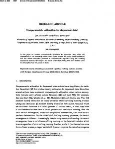
The results of the simulation study are summarized in Figures 1 and 2. The parameter of interest was X2 = var (X ). The mean squared errors depicted in the gures were obtained by averaging over 500 independent simulations, using B = 500 bootstrap resamples within each simulation. The bandwidth chosen for each simulation was h = b?1=5^ , where ^ was the sample standard deviation of the simulated sequence. (Except for the fact that the constant is 1 rather than 1:06, this is the \equivalent Normal density" prescription for bandwidth selection; see Silverman (1986, p. 45).) As before, we write l for block length. Let MSEm and MSEo denote the mean squared errors of the matched and ordinary block bootstrap methods, respectively. The following features emerged from our simulation study. Most importantly, the minimum mean squared error was consistently smaller under the matched block bootstrap than under the ordinary block bootstrap. As predicted by our theory, the block length at which the minimum occurred tended to be smaller for the matched block bootstrap. For example, in the case of Model 1 with (; n) = (0:80; 1000), the smallest value of MSEm was 4:0  10?6 and occurred at l = 5, whereas the smallest value of MSEo was 7:1  10?6 and occurred at l = 35. (Both values of l are correct to the nearest multiple of 5.) The bias terms were consistently negative for both methods. Note particularly that these trends were also apparent in Model 1 where the dependence was relatively long-range. In the case of the ordinary block bootstrap, optimal block length showed a marked tendency to increase with increasing range of dependence. This trend was not re ected in the matched block method, however. Similar results, not reported here, were obtained in simulations from a third model, a 9

moving average with negative coecient: Xt = at?1 + bt, where a = ?b = 2?1=2. This has (1) < 0 and (i) = 0 for i  2, and is \repulsive" in the sense that no covariance other than the variance is positive and thus 1 < 0. But (3.8) shows that 2 = 1=2. So kernel matching is expected to reduce bias which is con rmed by our simulations. Indeed, the only essential dierence noted between results in this and the other two models was that here, all biases were positive. As before, the minimum mean squared error was smaller for the matched block bootstrap than for the ordinary block bootstrap.

5 THEORETICAL RESULTS We now turn to rigorous derivation of results (3.2) and (3.3). The technical details of theory for block-matching are particularly arduous. To keep them in manageable, succinct form we treat a somewhat abstract version of the procedure that we earlier discussed in Sections 2 { 4. For simplicity we assume that n = bl for integers b (the number of blocks) and l (the length of each block). We consider the case where time series data fXi g are derived by sampling a continuous process with a sampling frequency which may increase with n. So, let fY (t); t 2 (0; 1)g denote a stationary stochastic process in continuous time, implying that   E fY (t)g does not depend on t, and (t)  cov fY (s); Y (s + t)g does not depend on s. Let  = (n) represent a sequence of positive constants possibly diverging to in nity as n increases, and put Xi = Y (i=). The strength of dependence of the process fXi g increases with increasing . Indeed, the variance of the sample mean is of order O(=n) (see below), and so long-range dependence might be considered to be characterized by the case where  increases with sample size. Our assumptions on the process Y are as follows: (C1A) Y is t0 -dependent for some t0 > 0, meaning that the sigma- elds F (0; s) and F (s + t0; 1) generated by fY (u); u 2 (0; s)g and fY (u); u 2 (s + t0; 1)g, respectively, are independent for each s > 0; (C1B)

E jY (t)j < 1 for some  > 8; to be determined later:

Condition (C1A) simpli es our arguments, but modi ed versions of our results hold in the case where Y is mixing with geometrically decreasing mixing rate. 10

Next we set down our assumptions on the block matching algorithm. Remember that p(j1; j2) for 1  j1 ; j2  b is the data-dependent probability that the next block is Bj2 , given that the current block is Bj1 . Put Vi = (Xi1; : : : ; Xir ) and Ui = (Xi;l?r+1; : : : ; Xil ), the rst r and the last r values in block i respectively. We impose the following conditions: (C2A) for all j1; j2,

p(j1; j2 ) = (Uj1 ; Vj2 ; Vj ; j 6= j2 );

where is nonnegative and symmetric in the last b ? 1 arguments, and r = O(); (C2B) for all j1,

b X j2 =1

(C2C) for some  > 0,

p(j1; j2 ) = 1;

sup E fp(j; j + 1)g = O(b?); j

(C2D) for any j1; j2 ; j3; j4 with j3 6= j2; j4 6= j2, there exists p0(j1; j2; j3; j4 ) 2 [0; 1] which depends only on Uj1 and Vj ; j 6= j3; j4 such that for some  > 0 and all 1  q < 1, sup kp(j1; j2) ? p0(j1; j2; j3; j4)kq = O(b?1?) ;

j1 ;j2 ;j3 ;j4

where jj:jjq denotes the Lq norm; (C2E) for some  > 0, ess supj2 6=j1+1 E fp(j1; j2)j Vj1 ; Bj ; j 6= j1; j1 + 1g = O(b?) : For example, we might de ne

p1(j1; j2) =

rY ?1 k=0

K f(Xj1 ;l?k ? Xj2 ;r?k )=hg ;

9 ,8 b 0; and 1  r = r(n) = o(). In the event that the denominator in the de nition of p(j1; j2) vanishes, de ne p(j1; j2 ) to equal b?1 for each value of j2 . Conditions (C2) may be veri ed in this setting, for a wide variety of processes including polynomial functions of Gaussian processes whose covariance

satis es (C1A). In this setting the approximating probability p0(j1; j2; j3; j4 ) in condition 11

(C2D) may be constructed by removing from the denominator in the de nition of p(j1; j2) a nite number of terms p1(j1; j ), so as to achieve the desired independence. Furthermore, condition (C2E) is an immediate consequence of the compact support of K and of the conditions imposed on h. Note that by way of contrast to rule (2.1), rule (5.1) now assumes strong positive dependence for neighbouring values, which is natural in the context of dense sampling of a continuous process. Of course, many alternative prescriptions of p are possible, still satisfying conditions (C2). In particular, there is considerable latitude for varying the block representatives that are compared via the kernel function in the de nition of p1 at (5.1). Let X and X  denote sample means of the data X and resampled data X , respectively; and let 8 9 nX ?1 < = 2 = 2(n) = var (X ) = n?1 : (0) + 2 (1 ? n?1j ) (j=); j=1

represent the variance of the sample mean. The matched-block bootstrap estimator of 2 is given by ^ 2 = var 0 (X ), where the prime denotes conditioning on X . To appreciate the size of the quantity that we are estimating, note that if  ! L as n ! 1, where 0 < L  1, then 8 n o > ?1 (0) + 2 P1 (j=L) if L < 1 < n j=0 2  > : 2(=n) R01 (t) dt if L = 1 : Therefore, 2 is of size =n. Let the stationary distribution on the block indices (1;


; b) be 1;


; b. Assume that the blocks Bi are produced with the chain in this stationary state, and put X 0 = P i X i , Xi = l?1 Pj Xij . Then E 0 (X ) = X 0 and ^ 2 = b?2(S1 + 2S2 ), where j

S1 = b S2 = = =

b X

i(X i ? X 0)2 ;

i=1 b?j bX ?1 X

j=1 i=1 bX ?1 i=1 bX ?1 i=1

 ? X 0 )g E 0f(Xj ? X 0)(X i+j

 ? X 0)g (b ? i) E 0 f(X 1 ? X 0)(X i+1

(b ? i)

b X b X j1 =1 j2 =1

j1 p(i; j1; j2 ) (X j1 ? X 0)(X j2 ? X 0)

and p(i; j1; j2) denotes the i-step transition probability in the Markov chain of blocks (p(1; j1; j2) = p(j1; j2 )). 12

If the stationary distribution of the block-matching rule is approximately uniform and is reached after two steps, then to a good approximation, Sj  Tj where

T1 =

b X (X i ? X )2 ; i=1

T2 =

b X b X j1 =1 j2 =1

p(j1; j2) (X j1 ? X )(X j2 ? X ) :

This suggests an alternative variance estimator,

~ 2 = b?2(T1 + 2T2 ) : We shall describe theory for this quantity. We believe that ~ 2 contains the essential features of ^ 2, for the following reasons. We showed earlier that the stationary distribution is uniform for a version of rank matching, and that it is approximately uniform in other cases since (3.6) is satis ed. That the stationary distribution is reached after two steps is plausible because Vj2 and Uj2 are independent if l is large. Hence, the two terms p(j1; j2) and p(j2; j3) are essentially independent. As the theorem below shows, the leading term in an expansion of bias is of size (nl)?12 , and equals ? 1 + 2 + o(2=nl) where

1  2(nl)?1

Z1

1 X i=1









i (i=) = 2=nl c1 + o 2=nl ;

c1  2 t (t) dt ; 0 2  2E fp(1; 3)(X 1 ? )(X 3 ? )g : We shall also show that 2 is typically of the same order as 1 .

Theorem 1. Assume conditions (C1) on the process Y , and (C2) on the matching rule, with  > max(8; 4=),  = o(l) and l = o(n). Then





n

o

E (~2) = 2 ? 1 + 2 + O n?2l + o 2 =(nl) ; o n var (~2) = 2n?1 l4 + o 2 n?3l + 4(nl)?2 :

(5.2) (5.3)

Since either 12 or n?1l4 dominates each remainder term then it is always true that

n

o

E (~2 ? 2)2  ( 1 ? 2 )2 + 2n?1l4 : If in addition l = of(n)1=2g and n2 = O(l3) then

E (~2) ? 2  ? 1 + 2 ; var (~2)  2n?1 l4: 13

(5.4)

The last result represents an analogue of (3.2) and (3.3). In order to compute the exact order of 2 and its leading term, we need stronger assumptions on the matching rules. A class of dierent rules is covered by

Theorem 2. Assume in addition to the conditions of the previous theorem that for some 1; 2 > 0, and all 1 < q < 1, kb p(1; 3) ? I (jX1l ? X31j  b?1 ) fP (jX1l ? X31j  b?1 jX1l )g?1kq = O(b?2 ) : Suppose too that  ! 1, Y is an almost surely continuous process and that Y (t) has a continuous density with respect to Lebesgue measure. Then

2 = 2 2=(nl) + of2 =(nl)g; where

2 =

l?1 0 X X i=?l+1 k=0

(5.5)

E fE [fY (i=) ? gjY (0)] E [fY (k=) ? gjY (0)]g?2:

If in addition the process Y is Gaussian, with (t) ? (0) = O(jtj) for some  > 0, then

2  c2 = 2 (0)?1

Z 1 0

2

(t) dt :

(5.6)

Remark 1. Observe that the rst-order contributions to squared bias and variance are

of sizes 4 (nl)?2 and 2 n?3l, respectively. Therefore the optimal block length is of size (n2 )1=3. Result (5.4) holds for such values of l.

Remark 2. As in Section 3, 2  c1 if Y is a Markov process. Remark 3. For a general stationary distribution i, X var (S1)  2 i24; so for (5.3) it seems necessary to have P 2  b?1. This implies, via the Cauchy-Schwarz i

inequality, that the stationary distribution is approximately uniform.

Remark 4. Without condition (C1A) we should replace the indices 1 and 3 in 2 by two indices j1 ; j2 with jj1 ? j2 j tending to in nity. Since then Bj1 and Bj2 become independent,

we obtain (3.7) from (3.4).

The eect of block matching on the bias may be studied most easily for Gaussian processes. Figure 3 depicts the asymptotic value of the ratio of the biases for matched 14

and non-matched blocks, 1 ? c2 =c1, for the covariance functions (t) = exp(?cjtj) (In this example we do not adhere to the technical assumption (C1A )). Here 0 <   2, and the larger  the smoother the process is. This example shows that the reduction in bias can be substantial. To appreciate that block-matching in terms of nearness of block ends is counter-productive for a time series with a considerable amount of repulsion, note that because c2 is always positive, block matching by nearness of block ends exacerbates the bias problem when c1 < 0. To be speci c, consider the case

8 > < (1 ? jtj) cos (!t) if jtj  1

(t) = > :0 otherwise ;

where ! is a parameter of the process. The value of c1 for this covariance function is 4!?3 sin ! ? 2!?2(1+cos !), which is negative for many choices of !. For !   the bias of the matched block estimator is substantially larger than the bias of the non-matched block bootstrap, see Figure 4. Similar behaviour is observed with other covariance functions that have negative parts. APPENDIX: PROOFS OF THEOREMS. Step 1: Preliminaries. Assume that E (Y ) = 0, and de ne

T3 =

b X 2

j=1

Xj ; T4 =

b X b X j1 =1 j2 =1

b X b X p(j1; j2 ) X j1 Xj2 ; T5 = p(j1; j2) X j2 :

 5 . Therefore, Since Pj2 p(j1; j2) = 1 then T2 = T4 ? XT

j1 =1 j2 =1

 5: ~ 2 = b?2(T3 + 2T4 ) ? b?1 X 2 ? 2b?2 XT It is straightforward to prove that

    E X 4 = O b?2 l?2 2 ;

and we shall show in Step 2 that for some  > 0,





o

n

E X 2 T52 = O b1? (=l)2 + b2? (=l)4 : With similar but simpler arguments one can show that

n

o

?
E X T5 = O l?1 + b1? (=l)2 : 15

(A.1)

In Step 3 we show that

 E (T4 ) = b2 E p(1; 3)X 1X 3 + O(=l) + O(b1? (=l)2):

(A.2)

Using an argument similar to that in Step 2 it may be proved that

n  o var (T4 ) = o b4 (=n)2 b?1 + l?2 2 :

From the bootstrap with independent blocks we know that

o

n

E (T3) = b2(l) = b22 (n) ? b2 1 + O (=l)2 ;

n

o

var (T3 )  2b3 4(n) = O b(=l)2 : These results, together with the Cauchy-Schwarz inequality and the fact that b = n=l, imply (5.2) and (5.3). Step 2: Proof of (A.1). Observe that





X E X 2 T52 = b?2 (6) E fp(j1; j2) p(j3; j4 )X j2 Xj4 Xj5 X j6 g = b?2 l?4S ;

where

S

X(10)

(A.3)

E fp(j1; j2) p(j3; j4)Xj2 k1 Xj4 k2 Xj5 k3 Xj6 k4 g ;

P P the six-fold sum (6) is over vectors (j1;


; j6) 2 f1;


; bg6, and the ten-fold sum (10) is over those vectors and also over (k1;


; k4) 2 f1;


; lg4 . We bound S by considering a number of dierent con gurations of the vectors (j1;


; j6 ) and (k1;


; k4). We call ki a boundary index if ki  r + t0  or ki  l ? r ? t0  + 1, and an interior index otherwise. The cases identi ed below cover all distinct con gurations up to isomorphisms. Since there is only a bounded number of the latter then we do not treat them here. Case I: k1;


; k4 are all interior indices. Here the term

E fp(j1; j2) p(j3; j4) Xj2 k1 Xj4 k2 Xj5 k3 Xj6 k4 g

(A.4)

factorizes into the product of E fp(j1; j2 ) p(j3; j4)g and E (Xj2 k1 Xj4 k2 Xj5 k3 Xj6 k4 ). The second factor equals zero unless (a) j2 = j4 = j5 = j6 , or (b) j2 = j5 6= j4 = j6, or (c) j2 = j4 6= j5 = j6, or one of the bounded number of possibilities isomorphic to these obtains. In subcase (a) the sum over k1;


; k4 contributes a term of order l2 2, and the sum 16

over j1; j2 and j3 contributes another O(b2). (Note that the sum of p(j1; j2 ) over its second index is identically 1.) Since the sums are in multiple then these two contributions should be multiplied together, and so the contribution to S obtained by summing the term at (A.4) over indices corresponding to subcase (a) is b2 l2 2 . The argument in subcase (b) is similar, with identical orders of magnitude arising from summation over k1;


; k4 and over j1 ;


; j4 . Therefore, the contribution to S that arises in subcase (b) is again O(b2 l2 2). The contribution to S from subcase (c) is

XXXX j1 j2 j3 j5





E fp(j1; j2) p(j3; j2)g O l2 2 :

(A.5)

In bounding the expectation we may suppose that j2 6= j3 + 1, since the contrary case may be treated more simply. (There, the number of sums in (A.5) is eectively only three, not four.) Under this assumption we may de ne p0(j1; j2 ; j3 + 1; j3 + 1) as in condition (C2D). Then,

E fp(j1; j2) p(j3; j2)g  E fjp(j1; j2 ) ? p0(j1; j2; j3 + 1; j3 + 1)j p(j3; j2)g +E fp0 (j1; j2 ; j3 + 1; j3 + 1) p(j3; j2)g: By the symmetry in condition (C2A), E fp(j3; j2)g  1=(b ? 1). Using (C2D) and choosing q > 2=, the rst term on the right is seen to be bounded by

    kp(j1; j2) ? p0(j1; j2; j3; j3)kq E fp(j3; j2)g1?(1=q) = O b?1? b?1+(1=q) = O b?1?(=2) :

Moreover, by (C2D) and (C2E), the second term on the right is bounded by

E [p0(j1; j2 ; j3 + 1; j3 + 1)E fp(j3; j2)jVj3 ; Bj ; j 6= j3 ; j3 + 1g]  Cb? E fp0(j1; j2; j3 + 1; j3 + 1)g  Cb? E fjp(j1; j2) ? p0(j1; j2; j3 + 1; j3 + 1)j + p(j1; j2)g  C 0 b?1? : Therefore, the expectation in (A.5) equals O(b?1?(=2)), and so the quantity at (A.5) equals O(b3?(=2)l22 ). Combining the results from subcases (a) to (c) we see that the contribution to S that arises from case I equals O(b3? l2 2), for some  > 0. Case II: k1;


; k4 are all boundary indices. De ning

 = (j1;


; j4) = p(j1; j2) p(j3; j4) ; 17

the term at (A.4) becomes E (Xj2 k1 Xj4 k2 Xj5 k3 Xj6 k4 ). We consider separately the subcases (a) j5 or j6 belongs to fj1 ? 1; j1 ; j2; j3 ? 1; j3; j4g, and (b) all other situations. In subcase (a) we bound the term by

n 

E =(?4)

o(?4)= 

E jXj2 k1 Xj4 k2 Xj5 k3 Xj6 k4 j=4

4=

:

In subcase (a) the number of values (j5; j6) is O(b) uniformly in (j1;


; j4), so summing over j5 and j6 gives a contribution O(b). By Holder's inequality

8 9 < X  =(?4)=(?4)= 0 X 14= @ 1A kk=(?4)  : E  ; j1 :::j4 j :::j4 j1 :::j4 8 9(1?4)= 8 thus ensures that this contribution does not exceed



O b4? 4



(A.6)

for some  > 0. Next we treat subcase (b). Let k3 and k4 be distant O() from (j5 ? 1)l + 1 and (j6 ? 1)l + 1, respectively. De ne

0 = 0(j1;


; j6) = p0(j1; j2; j5; j6 ) p0(j3; j4; j5; j6 ) : Then we have, in view of the independence of Xj5 k3 Xj6 k4 and 0Xj2 k1 Xj4 k2 ,

jE (Xj2k1 Xj4 k2 Xj5 k3 Xj6 k4 ) ? E (Xj2 k1 Xj4 k2 ) E (Xj5 k3 Xj6 k4 )j  jE f( ? 0)Xj2 k1 Xj4 k2 Xj5 k3 Xj6 k4 gj   +E X12 jE f( ? 0)Xj2 k1 Xj4 k2 gj :

(A.7)

By Holder's inequality, the rst term on the right-hand side of (A.7) is bounded by k ? 0 k=(?4) kX1k4 . Since

 ? 0 = p(j1; j2) fp(j3; j4) ? p0(j3; j4; j5; j6 )g +p(j3; j4) fp(j1; j2) ? p0 (j1; j2 ; j5; j6)g ?fp(j1; j2 ) ? p0(j1; j2; j5 ; j6)g fp(j3; j4) ? p0(j3; j4; j5; j6 )g ; 18

then the triangle inequality, Holder's inequality and condition (C2D) imply that for any  > 1,

n o k ? 0k=(?4) = O(b?1?) kp(j1; j2)k=(?4) + kp(j3; j4 )k=(?4)  ?2(1+) :

+O b

Similarly, the second term on the right-hand side of (A.7) is bounded by

 n k ? 0k=(?2) kX1k2 kX1 k22 = O b?1? kp(j1; j2 )k=(?2)  o  + kp(j3; j4)k=(?2) + O b?2(1+) :

If k3 is within distance O() of j5 l then we argue as above but with the de nition of 0 altered to p0(j1; j2; j5 + 1; j6) p0(j3; j4; j5 + 1; j6). Thus, the bounds just derived hold for any of the terms arising in subcase (b) of case II. Moreover, E (Xj5 k3 Xj6 k4 ) = 0 unless jj5 ? j6j  1. This, together with (A.7) and the bounds above, produce the following bound for the contribution to S from case II, subcase (b):

O(b4)

X  k(j1; j2; j3; j4 )k=(?2) + O b4?(1+) 4 kp(j1; j2 )k=(?4) j1 ;


;j4 j1 ;j2  6?2(1+) 4  X

+ O b

 :

Arguing as in the derivation of the bound at (A.6) we see that this equals





O b3+(4=) 4 + b5+(4=)??(1=) 4 + b4?2 4 ; which, since we made the assumption  > 4=, may be rendered of the order at (A.6) by choosing  > 1 suciently close to 1. Adding the bounds from subcases (a) and (b) we see that the total contribution to S from terms considered under case II is of the order at (A.6). Case III: Three ki's are boundary indices and the other is interior. Here the contribution to S is identically zero. The methods used to derive the bounds in Cases IV{VII below are somewhat dierent, and are given only in barest outline here. Although the bounds are identical, none of the cases is isomorphic to another. Case IV: k1; k2 are boundary indices and k3; k4 are interior. The contribution is identically zero unless j5 = j6, and there the contributions from the sums over (k3; k4); (k1; k2); j5 and (j1; j2; j3; j4) 19

are respectively O(l), O(2), O(b) and O(b2(?2)= b4(2=)). Multiplying them together we see that the total contribution to S is O(b3+(4=) l3 ). Because  > 8 and the geometric mean is bounded by the arithmetic mean, we have that b3+(4=)l3 = O(b3? l2 2 + b4? 4 ) for some  > 0. Case V: k3; k4 are boundary indices and k1; k2 are interior. The contribution to S is identically zero unless j2 = j4, and the contribution from the latter source is O(b4? l3 ) for some  > 0, using an argument similar to that employed to treat subcase (c) of Case I. Case VI: k1; k3 are boundary indices and k2; k4 are interior indices. The contribution to S is identically zero unless j4 = j6, and the contribution from the latter source is O(b3+(4=) l3 ). Case VII: k4 is a boundary index and the others are all interior. The contribution to S is identically zero unless j2 = j4 = j5, and the contribution from the latter source is O(b3+(1=) l3 ). Case VIII: k2 is a boundary index and the others are all interior. The contribution to S is identically zero unless j2 = j5 = j6, and the contribution from the latter source is O(b2+(2=) l3 ). Now we add the bounds derived in each of the eight cases. Because  > 8 and the geometric mean is bounded by the arithmetic mean, b3+(4=)l3 = O(b3? l22 + b4? 4 ) for some  > 0. Hence we obtain that for some  > 0,





S = O b3? l2 2 + b4? 4 : Result (A.1) now follows from (A.3). Step 3: Calculation of E (T4 ). Note that by symmetry, E fp(j1; j2 ) X j1 Xj2 g is the same for any j1 < b; j2 < b; jj2 ? j1j > 1. By an argument similar to that in Step 2 we may show that for any j1; j2,

n o jE fp(j1; j2) X j1 Xj2 gj = O(=l) E fp(j1; j1)g j1 ;j2 + O (=l)2 kp(j1; j2)k=(?2) :

Since p(j1; j2)  1 then

kp(j1; j2)k=(?2)  [E fp(j1; j2)g](?2)= : Using the fact that E fp(j1; j2)g  1=(b ? 1) if j2 6= j1 +1, and condition (C2C) if j2 = j1 +1, we obtain for  > 8,

n

o

E (T4) ? b2E fp(1; 3) X1 X 3g = O(=l) + O (=l)2 b1?3=4 ; 20

which is (A.2). Step 4: Proof of (5.5) and (5.6). Let Y; Y1 ; Y2 be independent processes with identical laws, and put Xl Zj = Yj (i=) : i=0

It is easy to see that under the conditions of Theorem 2,





2 = b?1 l?2 E [E fZ1 Z2 jY1(0) = Y2 (0)g] + o 2 =bl2 ; which is (5.5). Finally, for a Gaussian process, E fY (i=)jY (0)g = (i=)= (0) Y (0), which gives (5.6).

REFERENCES BU HLMANN, P. (1994). Blockwise bootstrapped empirical processes for stationary sequences. Ann. Statist. 22, 995{1012. BU HLMANN, P. AND KU NSCH, H.R. (1994). Block length selection in the bootstrap for time series. Research Report No. 72, Seminar fur Statistik, ETH Zurich. BU HLMANN, P. AND KU NSCH, H.R. (1995). The blockwise bootstrap for general parameters of a stationary time series. Scand. J. Statist., 22, 35 { 54. CARLSTEIN, E. (1986). The use of subseries values for estimating the variance of a general statistic from a stationary sequence. Ann. Statist. 14, 1171{1179. DAVISON, A.C. AND HALL, P. (1993). On Studentizing and blocking methods for implementing the bootstrap with dependent data. Aust. J. Statist. 35 215{224. EFRON, B. (1979). Bootstrap methods: another look at the jackknife. (With discussion.) Ann. Statist. 7, 1{26. EFRON, B. AND TIBSHIRANI, R.J. (1993). An Introduction to the Bootstrap. Chapman and Hall, New York. GO TZE, F. AND KU NSCH, H.R. (1993). Second order correctness of the blockwise bootstrap for stationary observations. Ann. Statist., under revision. HALL, P. (1985). Resampling a coverage pattern. Stoch. Proc. Appl. 20, 231{246. 21

HALL, P. AND JING, B. (1994). On sample re-use methods for dependent data. Research Report No. SR8{94, Centre for Mathematics and its Applications, Australian National University. HALL, P., HOROWITZ, J.L. AND JING, B. (1995). On blocking rules for the block bootstrap with dependent data. Biometrika 82, 561{574. KU NSCH, H.R. (1989). The jackknife and the bootstrap for general stationary observations. Ann. Statist. 17, 1217{1241. LAHIRI, S.N. (1993). On Edgeworth expansions and the moving block bootstrap for Studentized M -estimators in multiple linear regression models. J. Multivar. Anal., to appear. NAIK-NIMBALKAR, U.V. AND RAJARSHI, M.B. (1994). Validity of blockwise bootstrap for empirical processes with stationary observations. Ann. Statist. 22, 980{994. POLITIS, D.N. AND ROMANO, J.P. (1992). A general resampling scheme for triangular arrays of -mixing random variables with application to the problem of spectral density estimation. Ann. Statist. 20, 1985{2007. POLITIS, D.N. AND ROMANO, J.P. (1994). The stationary bootstrap. J. Amer. Statist. Assoc. 89, 1303{13. POLITIS, D.N. AND ROMANO, J.P. (1995). Bias-corrected nonparametric spectral estimation. J. Time Series Anal. 16, 67{103. SHAO, Q.M. AND YU, H. (1993). Bootstrapping the sample means for stationary mixing sequences. Stoch. Proc. Appl. 48, 175{190. SILVERMAN, B.W. (1986). Density Estimation for Statistics and Data Analysis. Chapman and Hall, London. WOOD, A.T.A. AND CHAN, G. (1994). Simulation of stationary Gaussian processes. J. Comp. Graph. Statist. 31, 409{432.

22

Figure 1: MSE comparisons for Model 1. Column panels correspond to  = 0:8, 0:95 respectively, and row panels to n = 200, 1000, 5000 respectively. The solid curve represents the matched block bootstrap, the dotted curve the ordinary block bootstrap.

0.0013

0.03

0.0012

0.028

0.0011

0.026

0.001

0.024 0.022

0.0008

MSE

MSE

0.0009

0.0007

0.02 0.018

0.0006

0.016

0.0005 0.0004

0.014

0.0003

0.012

0.0002

0.01 0

5

10

15

20

25

30

35

40

0

5

10

15

Block Length (l)

20

25

30

35

40

Block Length (l)

7e-05

0.0012 0.0011

6e-05 0.001 0.0009

5e-05

0.0008 MSE

MSE

4e-05

3e-05

0.0007 0.0006 0.0005

2e-05

0.0004 0.0003

1e-05 0.0002 0

0.0001 0

20

40

60

80

100

120

140

160

180

200

0

20

40

60

Block Length (l)

80

100

120

140

160

180

200

140

160

180

200

Block Length (l)

1.2e-06

5e-05 4.5e-05

1e-06

4e-05 3.5e-05

8e-07

MSE

MSE

3e-05 6e-07

2.5e-05 2e-05

4e-07

1.5e-05 1e-05

2e-07

5e-06 0

0 0

20

40

60

80

100

120

140

160

180

200

Block Length (l)

0

20

40

60

80

100

120

Block Length (l)

23

Figure 2: MSE comparisons for Model 2 when c = 0:00015. Column panels correspond to  = 1:5, 1:95 respectively; row panels to n = 1000, 5000 respectively. The solid curve represents the matched block bootstrap, the dotted curve the ordinary block bootstrap.

9e-07

1e-06

8e-07

9e-07

7e-07

8e-07

6e-07 MSE

MSE

7e-07 5e-07

6e-07 4e-07 5e-07

3e-07

4e-07

2e-07 1e-07

3e-07 0

20

40

60

80

100

120

140

160

180

200

0

20

40

60

Block Length (l)

80

100

120

140

160

180

200

700

800

900

1000

Block Length (l)

4e-08

4.5e-08

3.5e-08

4e-08 3.5e-08

3e-08

3e-08

MSE

MSE

2.5e-08 2e-08

2.5e-08 2e-08

1.5e-08 1.5e-08 1e-08

1e-08

5e-09

5e-09

0

0 0

100

200

300

400

500

600

700

800

Block Length (l)

0

100

200

300

400

500

600

Block Length (l)

24

0.6 0.4 0.0

0.2

(-c1+c2)/(-c1)

0.8

1.0

Figure 3: The gure depicts values of the ratio 1 ? c2 =c1 , the ratio of the bias of the matched to the bias of the non-matched block bootstrap, for Gaussian processes with (t) = exp(?cjtj ), where 0 <   2; the ratio is independent of c.

0.0

0.5

1.0 α

1.5

2.0

-0.1

Non-matched Matched

-0.3

Bias

0.0

0.1

Figure 4: The gure depicts values of ?c1 and of (?c1 + c2 ), the leading terms of the bias of the non-matched and matched block bootstrap, respectively, for the case (t) = (1 ? jtj) cos(!t)1fjtj