MATH FRAMEWORK FOR DECISION MAKING IN INTELLIGENT ...

Copyright by Pradeepkumar Ashok 2007

The Dissertation Committee for Pradeepkumar Ashok certifies that this is the approved version of the following dissertation:

MATH FRAMEWORK FOR DECISION MAKING IN INTELLIGENT ELECTROMECHANICAL ACTUATORS

Committee:

Delbert Tesar, Supervisor John Wesley Barnes Benito Fernandez Richard H Crawford Siddharth Pratap Si-Zhao Qin


by Pradeepkumar Ashok, B.Tech. ; M.S.

Dissertation Presented to the Faculty of the Graduate School of the University of Texas at Austin in Partial Fulfillment of the Requirements for the Degree of

Doctor of Philosophy

The University of Texas at Austin May 2007

Dedication I dedicate this work to my parents S.P. Ashok Kumar and Ambika Ashok and my beautiful wife Nishamathi Kumaraswamy

Acknowledgement I wish to thank Prof. Delbert Tesar for being my supervisor, guiding me in my research and supporting me financially during the course of my research. I consider myself very lucky to have been tutored by a visionary. Optimism and persistence are the other things that I learned from him during the course of my research under his guidance. I would also like to acknowledge the support of my colleagues Ganesh Krishnamoorthy, Thomas Yun, Jagadish Janardhan and Phani Kiran who do research relating to actuator intelligence for allowing me to bounce ideas off them and for giving me valuable feedback on the topic. I would like to thank the Robotics Reseach Group management team Chetan Kapoor, Mitch Pryor, Janie Terrel and Betty Wilson for providing an atmosphere conducive to research. I would like to thank Kyogun Chang for his support and guidance that was instrumental in my doing well in the Ph.D. qualifier exam. I would like to thank my parents for supporting me through these years and being very patient with regards to the amount of time I spent getting my education. I thank them for impressing upon me the need for higher education. I also want to thank my beautiful and intelligent wife for her support. I started writing my proposal after I was introduced to her and consider her to the key factor in my being focused and having made it out of graduate school with a sense of accomplishment.

v


Publication No._____________

Pradeepkumar Ashok, Ph.D. The University of Texas at Austin, 2007

Supervisor: Delbert Tesar Significant progress has been made in the science of designing sophisticated electromechanical actuators to serve the ever growing needs of complex motion. There are many controllable parameters that can be managed in an actuator in real time to obtain significant operational benefits. However, normally only one parameter (usually current) is managed in real time. The focus has not been managing the available resources to maximize performance but on traditional control for stability. Actuators are very nonlinear and the operation of an actuator is full of uncertainties. The nonlinearity is trivialized by using simplified linear control. The uncertainties are also neglected. Actuators are often discarded before they have been fully utilized for lack of reliable knowledge with regards to the actual condition (degradation) of the actuator. Here we strive for the best operational

vi

decision or course of action. Optimization is definitely one way to tackle this problem. But that approach, for the most part, is not transparent to the end user who might like to have some assurance that the decisions suggested by these optimization algorithms are not flawed. The objective of this report is to develop a math framework for decision making in actuators to overcome the previously cited obstacles. The framework should allow for human involvement in the decision making process. It should use test data models (as opposed to simple physics based models) for maximum utilization of actuator capabilities and representation of the nonlinearities. The model should be updatable as new information about the actuator is obtained from a sensor suite. The framework should be capable of handling uncertainties in the parametric model, the in-situ sensor data and the decision process itself. It should allow the generation and full utilization of decision making criteria for performance maximization, condition based maintenance, fault tolerance, layered control and force motion control. Based on the above requirements a framework was developed in this report that requires the following math techniques; Bayesian causal network modeling of actuators, design of experiments for data collection, Bayesian regression for model fitting, Sensor data fusion techniques for accurate modeling, combining maps to obtain decision surfaces and applying norms on the decision surfaces We show that Bayesian causal network modeling is the best suited for our task. It offers the advantage of isolating only those parameters that are important during the operation of the actuator.

vii

Also it enables the inclusion of uncertainties and propagation of uncertainties

to

demonstrate

how

other

parameters

Bayesian

through

regression

causal

techniques

links. make

We it

straightforward to update the model when new data becomes available and how this in turn helps condition based maintenance. Using the actuator Bayesian causal network we then generate 3 dimensional decision surfaces. We illustrate eight different ways of arriving at these decision surfaces from primary performance maps (maps that were generated through experiments). The illustrations were done using data gathered on a test bed built specifically for the purpose of developing the decision making framework. The test bed is modular and has a controller architecture that allows for different types of actuators (with any type of prime mover; switched reluctance motors, brushless DC motors, brushed DC motors and stepper motors) to be tested on it. We then proceed to develop norms mathematically. They are applied to the decision surfaces and their physical meaning is brought out through example scenarios. The framework was demonstrated on a simple actuator model and found to work satisfactorily for performance maximization and condition based maintenance. In future, the framework needs to be further developed to treat specific decision making situations relating to fault tolerance, layered control and force/motion control.

viii

TABLE OF CONTENTS 1

Introduction.................................................................................1 1.1

The Intelligent Actuator...........................................................1

1.2

Operation of an Intelligent Actuator ........................................2

1.3

Framework for Decision Making: Brief Background................3

1.4

Problem Statement and Research Objective..........................5

1.5

Report Outline ........................................................................8

1.6

Conclusion..............................................................................9

2

Literature Review…………………… ........................................11 2.1

Introduction...........................................................................11

2.2

Electro-Mechanical Actuator Architecture.............................11

2.3

Review of Components of the Framework............................13

2.3.1

Modeling of Actuators....................................................13

2.3.2

Propagating Uncertainties .............................................26

2.4

Performance Maps ...............................................................30

2.4.1

History of performance maps ........................................31

2.4.2

Mathematical Definition .................................................31

2.4.3

Performance Maps for Actuators...................................34

2.5

Performance Envelopes .......................................................38

2.6

Performance Criteria ............................................................41

2.7

Control Via Criteria Based Decision Making.........................43

2.8

Conclusion............................................................................44

3

Overview of Decision Making Framework .............................46 3.1

Introduction...........................................................................46

3.2

Causal Networks ..................................................................46

3.3

Probabilistic Models..............................................................51

ix

4

3.4

Generating Maps ..................................................................54

3.5

Generating Envelopes ..........................................................60

3.6

Decision Making ...................................................................62

3.7

Chapter Summary ................................................................64

Bayesian Mathematics…………….. .........................................65 4.1

Introduction...........................................................................65

4.2

Bayesian Causal Network ....................................................65

4.2.1

Causal Network .............................................................66

4.2.2

Bayesian Belief Network ...............................................67

4.2.3

Causal Network to Bayesian Causal Network ...............72

4.3

Bayesian Regression............................................................76

4.3.1

Bayes Theorem .............................................................78

4.3.2

Bayesian Linear Regression .........................................79

4.3.3

Bayesian Non Linear Regression ..................................88

4.4 5

Chapter Summary ................................................................91 Uncertainty Propagation…......................................................92

5.1

Introduction...........................................................................92

5.2

Discretization........................................................................92

5.3

Uncertainty Propagation .......................................................95

5.3.1

Forward Propagation.....................................................96

5.3.2

Backward Propagation ..................................................97

5.3.3

Propagation in Polytree Structures..............................100

5.3.4

Clustering Algorithm ....................................................105

5.4

Adding Probability Density functions ..................................106

5.5

Chapter Summary ..............................................................110

6

Performance Maps………… ..................................................111 6.1

Introduction.........................................................................111

x

6.2

Model..................................................................................111

6.3

Test bed .............................................................................112

6.4

Collecting Data for the Model .............................................115

6.5

Creation of Secondary Performance Maps.........................122

6.5.1

Additive Combination ..................................................122

6.5.2

Causal Flow Combination ...........................................131

6.5.3

End Task Combination ................................................137

6.5.4

Uncertainty Combination .............................................144

6.5.5

Region Partition Combination......................................147

6.5.6

Control Parameter Combination ..................................150

6.5.7

Envelope Generation Combination..............................155

6.5.8

Multiplicative Combination...........................................159

6.6 7

Chapter Summary ..............................................................164 Norms………………………. …. ..............................................166

7.1

Introduction.........................................................................166

7.2

Norm for Maps....................................................................166

7.2.1

Maximum: NORM _ MAX ( Z , X , Y ) ...............................167

7.2.2

Probability: NORM _ PROB( Z L ≤ Z ( X i , Y j ) ≤ ZU ) ..........170

7.2.3

Minimum: NORM _ MIN ( Z , X , Y ) .................................172

7.2.4

Difference: NORM _ DIF ( Z Old , Z New ) ............................173

7.2.5

Range: NORM _ RANGE ( Z , X , Y ) ................................175

7.2.6

Volume: NORM _ VOL( Z , X , Y ) ....................................176

7.2.7

Root Mean Square: NORM _ RMS ( Z , X , Y ) .................179

7.2.8

Volatility: NORM _ VOLAT ( Z , X , Y ) ..............................182

7.2.9

Monotonicity: NORM _ MONOT ( Z , X , Y ) .....................185

xi

7.2.10 7.3 8

Power Mean: NORM _ POW p ( Z , X , Y ) ........................188

Chapter Summary ..............................................................190 Conclusion…………………. ...................................................193

8.1

Introduction.........................................................................193

8.2

Decision Making in Intelligent Actuators .............................196

8.2.1

Modeling Nonlinearities and Uncertainties ..................197

8.2.2

Criteria Based Decision Making ..................................212

8.2.3

Software and Test Bed Development..........................230

8.3 A

Conclusion..........................................................................243 Appendix: Test Bed ..……………………………………………247

A.1

Switched Reluctance Motor………………………………….247

A.2

Controller (H-Bridge Amplifier)…..…………………………..251

A.3

PXI Chassis………………………………………..…………..253

A.4

PXI Embedded Controllers…………………………….…… 254

A.5

FPGA Board………………………………………………..….255

A.6

Hardware Programming Architecture…………..…………...256

A.7

Data Acquisition Card……………..………………………….257

A.8

Radio Shack Digital Sound Level Meter……………………258

A.9

Torque Transducer……………………………………….…..259

A.10

Power Supply………………………………………………….260

A.11

Current Sensor………………………………………………..261

B

Appendix: LabVIEW Program for SRM………………………..262

C

Appendix: Additive Combination C#......................................268

D

Appendix: Software Development Plan……………………….272 References…………………………………………………………274 Vita…………………………………………………………………..284

xii

LIST OF FIGURES Figure 1-1 System Level and Actuator Level Decision Making .............4 Figure 1-2 Example of Decision Surface [Hvass and Tesar, 2004].......6 Figure 2-1 Performance Maps [Omekanda, 2003].............................17 Figure 2-2 Global Performance Map (Torque, Drive Efficiency and Torque Ripple Combined) [Omekanda, 2003] ............................18 Figure 2-3 Example of a Neural Network ............................................21 Figure 2-4 Uncertainty Due to Noise...................................................23 Figure 2-5 Modeling Uncertainty.........................................................24 Figure 2-6 Avoiding Overfitting ...........................................................25 Figure 2-7 Models Relating Parameters .............................................26 Figure 2-8 Bayesian Network (Automotive Engine Start) [Thiesson et. al, 2002].......................................................................................28 Figure 2-9 Amplifier Performance Map ...............................................36 Figure 2-10 Motor Performance Map [Reinert, J., et.al, 1998] ............36 Figure 2-11 Bearing Performance Map [Tesar and Vaculik, 2005] .....37 Figure 2-12 Gear Train Performance Map [Podra and Andersson, 2000]............................................................................................37 Figure 2-13 Conceptual Visualization of Performance Envelopes (Yoo and Tesar, 2002) .........................................................................40 Figure 2-14 Conceptual Illustration of Criteria-Based Control Law .....43 Figure 3-1 Overview of the Steps for Decision Making in Actuators ...47 Figure 3-2 Preliminary Causal Network of Actuator Operation Parameter....................................................................................50 Figure 3-3 Causal Network of Switched Reluctance Motor.................52 Figure 3-4 Causal Network Showing the Combination of Noises........53

xiii

Figure 3-5 Plot of Tangential Flux density versus Turn on and Turn off angle............................................................................................55 Figure 3-7 Generating Maps ...............................................................57 Figure 3-7 Plot of Torque Versus Turn-on angle and Turn-off angle (Current = 1 amp) ........................................................................58 Figure 3-8 Configuration to generate Map no. 19 (MSPD Versus MTOR and MLOD) ......................................................................59 Figure 3-9 Configuration to generate Map no. 20 (MSPD Versus MTFD and MLOD) ..................................................................................59 Figure 3-10 Torque Envelope .............................................................60 Figure 3-11 Torque - Speed - Efficiency Envelope [Hvass & Tesar, 2004]............................................................................................63 Figure 3-12 MNOI (Normalized) versus MTON and MTOF ................64 Figure 4-1 An Example of a Bayesian Network and Conditional Probability Tables ........................................................................68 Figure 4-2 Causal Chain .....................................................................70 Figure 4-3 Common Causes...............................................................70 Figure 4-4 Common Effects ................................................................71 Figure 4-5 Direct and Indirect Relations .............................................73 Figure 4-6 Circular loop in Causal Network ........................................75 Figure 4-7 Elimination of Circular loop................................................76 Figure 4-8 Functions Representing the Bayesian Causal Network.....77 Figure 4-9 Histograms of the Data used in Regression Example .......82 Figure 4-10 Plot of Regression Model ................................................85 Figure 4-11 Bayesian Linear Regression of y=ax+b+σ.......................89 Figure 5-1 Bayesian Causal Network .................................................93 Figure 5-2 The Distribution of Torque for Current = 2 amps ...............94

xiv

Figure 5-3 Polytree Bayesian Causal Network .................................100 Figure 5-4 Polytree with Evidence ....................................................101 Figure 5-5 Parents and Children of node Ni ......................................102 Figure 5-6 Ad hoc Clustering ............................................................105 Figure 6-1 Actuator Model ................................................................112 Figure 6-2 The Test Bed ...................................................................113 Figure 6-3 The Generalized Controller .............................................114 Figure 6-4 Schematic Diagram of Test Bed ......................................116 Figure 6-5 PWM Signal.....................................................................118 Figure 6-6 Current Profile Caused by Different PWM Signals ..........119 Figure 6-7 MSPD Versus GSPD.......................................................121 Figure 6-8 GLOS Versus GSPD and ALOD .....................................121 Figure 6-9 Distribution for GLOS corresponding to MPDC=6 and MPFR=2 ....................................................................................126 Figure 6-10 Additive Combination of Maps.......................................127 Figure 6-11 Uncertainty Band for Gear Loss ....................................128 Figure 6-12 Distribution for MLOS corresponding to MPDC=6 and MPFR=2 ....................................................................................128 Figure 6-13 Uncertainty Band for Motor Loss ...................................129 Figure 6-14 Uncertainty Band for Total Loss ....................................130 Figure 6-15 Causal Flow Combination..............................................132 Figure 6-16 MTOR Versus MPDC and MPFR ..................................133 Figure 6-17 GTOR Versus MTOR ....................................................133 Figure 6-18 GSPD Versus GTOR and ALOD ...................................134 Figure 6-19 GNOI Versus GSPD and ALOD ....................................134 Figure 6-20 GNOI Versus MPDC and MPFR (For different ALODs) 135

xv

Figure 6-21 GNOI Versus MPDC and MPFR (For different ALODs) (With Uncertainty Bounds).........................................................136 Figure 6-22 MNOI Versus MPDC and MPFR ...................................137 Figure 6-23 Normalized MTOR versus MPDC and MPFR................139 Figure 6-24 Normalized MLOS versus MPDC and MPFR ................140 Figure 6-25 Normalized MNOI versus MPDC and MPFR .................141 Figure 6-26 Maximizing Torque and Minimizing Loss.......................142 Figure 6-27 Maximizing Torque and Minimizing Noise .....................143 Figure 6-28 Normalized Uncertainty of Motor Torque.......................144 Figure 6-29 Normalized Uncertainty of Motor Loss...........................145 Figure 6-30 Combined Uncertainty Map ...........................................145 Figure 6-31 Uncertainty Bounds on the Combined Map (Refer Figure 6-26) ..........................................................................................146 Figure 6-32 Normalized Maps Superimposed in the Same Map.......148 Figure 6-33 Combined Map Demonstrating that Different Parameters dominate Different Operational Regions....................................148 Figure 6-34 Projected View of the Combined Map ...........................149 Figure 6-35 GNOI Versus MTON and MPDC (for different values of MPFR) .......................................................................................151 Figure 6-36 GNOI Versus MTON and MPFR (for different values of MPDC).......................................................................................151 Figure 6-37 GNOI Versus MTON and (MPDC and MPFR)...............153 Figure 6-38 GNOI Versus MTON and MPDC (The combined surface and the different layers for the different values of MPFR)..........153 Figure 6-39 GNOI Versus MTON and MPFR (The combined surface and the different layers for the different values of MPDC) .........154 Figure 6-40 GLOS Versus MPFR (Envelope) ...................................156

xvi

Figure 6-41 GLOS Versus MPFR and MPDC (Envelope) ................157 Figure 6-42 MTOR Versus MPDC and MPFR ..................................160 Figure 6-43 MSPD Versus MPDC and MPFR ..................................160 Figure 6-44 MPOW Versus MPDC and MPFR .................................163 Figure 7-1 Performance Map to Demonstrate Maximum Norm ........169 Figure 7-2 Performance Map demonstrating the use of the Certainty Norm..........................................................................................171 Figure 7-3 Example demonstrating use of Difference Norm [Hvass & Tesar, 2004] ..............................................................................174 Figure 7-4 Efficiency versus Torque and Speed Maps [Hvass and Tesar, 2004] ..............................................................................178 Figure 7-5 GNOI versus MPDC and MTON (MPFR=11KHz) ...........179 Figure 7-6 GNOI versus MPDC and MTON (MPFR=20KHz) ...........180 Figure 7-7 GNOI versus MPDC and MTON (MPFR=14KHz) ...........181 Figure 7-8 GNOI versus MPDC and MTON (MPFR=14KHz) ...........181 Figure 7-9 Plot of MTOR versus MTON............................................183 Figure 7-10 Increase in Volatility due to Sensor Faults.....................184 Figure 7-11 Normalized MLOS versus MPDC and MPFR ................187 Figure 7-12 Maximizing Torque and Minimizing Loss.......................187 Figure 7-13 Maximizing Torque and Minimizing Noise .....................188 Figure 7-14 BLIF versus BSPD and BLOD .......................................189 Figure 8-1 Actuator Decision Making Framework .............................195 Figure 8-2 Simple Actuator Bayesian Causal Network .....................200 Figure 8-3 Probability Distribution of MLOS corresponding to MPDC=6 , MPFR =2 and MTON =0............................................................202 Figure 8-4 Simple Causal Network ...................................................203 Figure 8-5 Bayesian Linear Regression of y=ax+b+σ.......................205

xvii

Figure 8-6 Preliminary Actuator Bayesian Causal Network ..............209 Figure 8-7 Sensor Fusion [Krishnamoorthy and Tesar, 2005] ..........211 Figure 8-8 Additive Combination of Performance Maps ..................214 Figure 8-9 End Task Combination (Torque and Loss) ......................216 Figure 8-10 End Task Combination (Torque and Noise) ..................217 Figure 8-11 GLOS Versus MPFR and MPDC (Envelope) ................219 Figure 8-12 Illustration of RMS Norm ...............................................223 Figure 8-13 Illustration of Monotonicity Norm ...................................224 Figure 8-14 Illustration of Multiple Paths Available to go from A to B228 Figure 8-15 Software Test Bed .........................................................232 Figure 8-15 Controller Architecture...................................................233 Figure 8-16 Data Handling and Movement for Actuator Management ..................................................................................................235 Figure 8-18 Preliminary Architecture of Actuator Decision Making Software [ Yun and Tesar, 2007] ...............................................238

xviii

LIST OF TABLES Table 2-1 Decision Making Requirements for the Different Actuator Classes [Tesar et.al., 2006] .........................................................14 Table 2-2 Criteria Space [Omekanda, 2003] ......................................18 Table 2-3 Comparison of Uncertainty Measures [Walley, 1996] .........29 Table 2-4 Performance Maps in the Automotive Industry ...................32 Table 2-5 Performance Maps for Different Actuator Components [Tesar, et.al., 2005]......................................................................39 Table 2-6 Actuator Criteria Developed at the Robotics Research Group ....................................................................................................42 Table 2-7 Summary of Literature Review ...........................................45 Table 3-1 Potential Map Alternatives for the SRM Causal Network....54 Table 4-1 Data for Regression Example.............................................81 Table 4-2 Least Squares Computation for Fitting ...............................85 Table 5-1 Conditional Probability Table ..............................................95 Table 5-2 CPT Example for Uncertainty Propagation .........................96 Table 5-3 Prior Beliefs for Current ......................................................98 Table 5-4 Joint Distribution for MTOR and MCUR based on Priors in Table 5-3 .....................................................................................99 Table 5-5 Discrete Probability Distributions ......................................108 Table 5-6 Variance of x.....................................................................109 Table 5-7 Expected Values and Variances of the Distributions ........109 Table 6-1 Test Bed Components ......................................................115 Table 6-2 Plots for the Actuator Model .............................................120 Table 6-3 Part of Conditional Probability Table for Equation 6.7 ......124 Table 6-4 Objectives for Combining Maps ........................................138

xix

Table 6-5 Probability Tables for MTOR and MSPD ..........................161 Table 6-6 Probability Distribution Table for MPOW ..........................162 Table 6-7 Probability Distribution Table for MPOW (Summarized) ...163 Table 6-8 Summary of the Different Combinations ...........................165 Table 7-1 Discrete Representation of a Performance Map ...............167 Table 7-2 Mean of Performance Map MTOR versus MPDC and MPFR ..................................................................................................169 Table 7-3 Standard Deviation of Performance Map MTOR versus MPDC and MPFR......................................................................169 Table 7-4 Norms to be applied on Decision Surfaces.......................192 Table 8-1 Main Topics of this Report ................................................194 Table 8-2 Functional Representation of the Actuator in Figure 8-2...201 Table 8-3 Norms to be applied on Decision Surfaces.......................221 Table 8-4 Summary of the Different Combinations ...........................226 Table 8-5 Comparison of the Different Platforms[Adapted from National Instruments, 2007].......................................................240 Table 8-6 One Year Action Plan for AMOS ......................................242 Table 8-7 Summary of Main Results.................................................245 Table 8-8 Summary of Main Results (Continued) .............................246

xx

LIST OF ABBREVIATIONS

MTON MTOF MCUR MLOAD MFDR MFDT MTOR MSPD MNOI MEFF MPOW MLOS MPDC MPFR GTOR GSPD GNOI GLOS ALOS BLIF BSPD BLOD TNOI TLOS

Motor Turn On Angle Motor Turn Off Angle Motor Current Motor Load Radial Flux Density Tangential Flux Density Motor Torque Motor Speed Motor Noise Motor Efficiency Motor Power Motor Loss Motor Switching Duty Cycle Motor Switching Frequency Gear Torque Gear Speed Gear Noise Gear Loss Actuator Load Bearing Life Bearing Speed Bearing Load Total Noise Total Loss

xxi

1 1. Introduction 1.1 The Intelligent Actuator This report describes a math framework for decision making in intelligent electromechanical actuators. To establish the need for this math framework we will first define what we mean by an intelligent actuator. An intelligent actuator has the following characteristics:

1. It has numerous sensors for situational awareness of multiple internal physical phenomena (sensor fusion). 2. It is capable of adapting its operation to different situational requirements (criteria based control). 3. It knows the limit of its performance at all times (awareness of its performance envelope). 4. It knows when it is time for maintenance (condition based maintenance). 5. It knows how to use redundancies within it to continue operation even after a fault has occurred (fault tolerance). 6. Given extra resources within itself, it can provide layered control (mixed physical scales) or a combination of force and motion (separate force and velocity priorities) 7. It can communicate effectively with humans (human oversight).

The above list was summarized from discussions of intelligence in actuators by Isermann and Ulrich [1993], Xie, Pu, and Moore [1998],

1

Yang and Clarke [1999] and reports written with the Robotics Research Group (RRG) at The University of Texas at Austin starting with Michaels and Tesar [1995].

1.2 Operation of an Intelligent Actuator These intelligent actuators can be operated with different levels of autonomy. 1. Fully Autonomous: The actuator makes all the decisions with regards to its operation.

This scenario is highly unlikely except in

situations where the environment is pretty stable and does not vary very much. An example would be an actuator in a mobile robot in a factory setting doing repetitive undemanding tasks. 2. Semi-Autonomous: Here there is a human in the loop who monitors the overall situation and operates the actuator using commands such as “go slow”, “go fast”, “conserve energy”, “operate quietly” etc. This kind of a situation might arise where a soldier is faced with having to defuse a bomb and needs to move the actuators in a robot using simple commands. These commands map to operational regimes with preset fused criteria. 3. Least Autonomous: Here also there is a human in the loop who monitors the overall situation.

However instead of controlling the

actuator using simple commands, the human uses performance maps and decision surfaces as a basis to instruct the actuator as to what the control parameters should be.

The weights for criteria fusion are

decided depending on the current operation scenario. This kind of a situation might arise where engineers and scientists are controlling a

2

mobile robot in a hostile environment such as Mars or deep-sea and operational certainty is needed to meet a particular objective.

1.3 Framework for Decision Making: Brief Background To operate an intelligent actuator in all the three modes of operation discussed in the previous section, we need an extensive body of algorithms. This report lays the groundwork for this. At the Robotics Research Group (RRG) at The University of Texas at Austin much work has been done on criteria based decision making for redundant robots at the system level over the last 20 years. Cleary and Tesar [1990] identify modeling of the robot and criteria as the basis for decision making in redundant robots (excess DOF). Van Doren and Tesar [1992] develop more than 25 criteria for decision making. Hooper and Tesar [1994] follow up on this and develop a generalized inverse kinematics solution methodology for redundant robots that makes use of the criteria previously developed. These methods and criteria that were developed at RRG were quickly implemented in a software framework called OSCAR [Kapoor and Tesar, 1996]. OSCAR stands for Operation Software Components for Advanced Robotics. Since then numerous reports have been written at RRG to advance decision making on the system level. The results of all of these reports have been implemented in OSCAR and OSCAR is today considered a mature product. The most notable of these later reports are the ones by Pryor and Tesar [2002] and Pholsiri and Tesar [2004] both of which tackled the question of criteria fusion for decision making.

3

SYSTEM LEVEL MODELING

ACTUATOR LEVEL MODELING

Kinematic Model Dynamic Model Compliance Model

Will be developed in this report Initial Set of Norms will be developed in this report

Norms

SYSTEM LEVEL CRITERIA EXAMPLES

ACTUATOR LEVEL CRITERIA EXAMPLES

Joint Range Availabilty Torque Limit Avoidance Smallest Minimum Distance

Torque Efficiency Noise

SYSTEM LEVEL CRITERIA FUSION TECHNIQUES

ACTUATOR LEVEL CRITERIA FUSION TECHNIQUES

Task Based Decision Making Critical Boundary Method

Will be developed in later report

Figure 1-1 System Level and Actuator Level Decision Making

4

While decision making on the system level is mature (left side of Figure 1-1) the same cannot yet be said for decision making on the actuator level. There is the lack of a suitable methodology for modeling the actuator, generating criteria and for criteria fusion when it comes to decision making. A lot of work has been focused on actuator criteria development.

Scott and Tesar [1999] mathematically defined 8

actuator performance criteria. Turner and Tesar [2000] added 16 more to this list of actuator performance criteria. Hvass and Tesar [2004] identified

3

performance

criteria

relevant

to

condition

based

maintenance. In all of these efforts however not much emphasis was given to arriving at a generalized method to model the intelligent actuator (something that was already available for system level robots) in a full architecture of internal resources. This stalled the development of a decision making software framework for actuators. Yoo and Tesar [2004] show the feasibility of using 3-D performance maps for interactivity in decision making. However the process of arriving at these 3-D performance maps needs to be streamlined The research here extends the above research by setting up the mathematical framework to create robust nonlinear models of the actuator and to use them for decision making in an interactive setting.

1.4 Problem Statement and Research Objective The problem that this report aims to tackle is the lack of generalized multi-criteria decision making architecture for actuators. Discussions with colleagues at the Robotics Research Group (RRG)

5

have led to the following list of requirements for the decision making system.

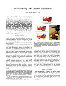
1. Should be visual and interactive: This is an absolute necessity when humans will be involved in decision making. The consensus was to use 3-D plots that we call performance maps / decision surfaces to communicate information about the actuator to the decision maker.

% Efficiency

Nominal Performance Condition Assessed Performance Condition Required Performance Condition

Speed (rad/sec)

Torque (Nm)

Figure 1-2 Example of Decision Surface [Hvass and Tesar, 2004]

Figure 1-2 is an example of the use of 3D maps for decision making [Hvass and Tesar, 2004]. It shows 3 surfaces. The one on the very top (nominal performance condition) is the performance surface of the motor in its as built condition. The surface in the middle (assessed performance condition) is generated after some faults were introduced into the motor (it shows degradation of the motor). The lower most

6

surface (required performance condition) is the absolute minimum acceptable performance. If the actuator performance goes below this surface then the actuator is replaced.

Hvass and Tesar [2004]

introduced calculable metrics (single number extracts from these surfaces) such as “Health Margin” and “Remaining Useful Life” to further help make decisions. Performance maps also help reduce mistakes that could be caused by blindly using optimization routines.

2. Use data from testing: Empirical models are more accurate than models derived purely from first principles. Therefore the framework must have the capacity to accommodate data procured from testing the actuator. There is often a fear that empirical models are black box models. However by using 3-D plots in the decision making process these empirical models become acceptable.

3. Be able to update model quickly: The ability to update the actuator model as and when new information becomes available is critical to condition-based maintenance.

4. Handle uncertainties: The framework should be able to handle uncertainties including uncertainty in sensor data, process uncertainty and modeling uncertainty.

5. Generate and combine performance maps to obtain decision surfaces: The framework should allow the easy generation of performance maps and decision surfaces with different parameters as

7

the X, Y and Z axes of the 3-D plots. It should allow for the easy generation of actuator criteria and also fusion of the criteria.

6. Should be modular: The decision making framework at the system level in RRG is modular. This made it possible to build an extensible software framework (OSCAR). Likewise, a modular decision making framework at the actuator level will make it easy to implement in software.

1.5 Report Outline In Chapter 1, we start by defining an intelligent actuator. We then describe the different modes by which an intelligent actuator is operated. Then we discuss decision making in system level robotics and compare it to the progress made in the actuator level. We finally present the problem statement and the objective of this report. In Chapter 2, we review the spectrum of actuators that make up an intelligent mechanical system. We review various actuator modeling techniques and provide an introduction to performance maps, envelopes and criteria. In Chapter 3, we outline the full decision making framework. Using an example we show how to model the actuator and use the model to generate performance maps / decision surfaces. We then show these decision surfaces help in making decisions. Chapter 4 discusses in more depth the modeling of an actuator using Bayesian causal networks for uncertainty propagation. We also

8

discuss the framework for the mathematical representation of empirical actuator data. Chapter 5 discusses algorithms for propagating uncertainties, in particular Pearl’s belief propagation algorithm. We also present a methodology for adding uncertainties, both in the continuous and the discrete domain. In Chapter 6, we show how to generate performance maps and how to combine them. We present 8 different ways to combine the maps. We illustrate each combination with an example. In Chapter 7, we mathematically define 10 different norms which are single value extracts from performance maps. These norms have physical meaning and help in decision making. We also present examples illustrating how these norms help in decision making Chapter 8 concludes the report and summarizes the complete framework. This is a standalone chapter and can be read by itself. Areas of future work are also discussed in this chapter.

1.6 Conclusion Actuators are highly nonlinear and their operational parameters drift due to aging and extended operation. Users want more performance from these actuators at lower cost and classical control theory is no longer sufficient to do this. Computational power has become cheaper allowing us now the opportunity to attempt to operate these devices closer to their operational margin using sophisticated algorithms thereby maximizing their performance. When operating actuators close to their operational margin, it is all the more important that the user be aware of the limits of the

9

actuator.

This necessitated a need for a new decision making

framework based on visual 3-D plot (performance maps/ decision surfaces). To be able to make decisions using these 3-D plots a framework was also needed to extract physically meaningful single value numbers from these maps (norms). The framework to generate decision surfaces and apply norms on them is the primary objective of this report. This report can only be considered a starting point. The framework will be demonstrated on performance maximization and condition based maintenance. Its use for fault tolerance, layered control and force/motion control will be left for future study. We call the actuators on which the framework is applied “Intelligent Actuators”. We started this chapter by discussing the characteristics of an intelligent actuator. We discussed 3 modes of operation for these actuators. The Robotics Research Group has 20+ years of experience in decision making on system level robotics. We briefly review them to show the general direction that the framework for actuators is headed. Towards the end of this chapter we defined the problem statement and the research objectives of this report.

10

2 2. Literature Review 2.1 Introduction In this chapter we will first introduce 10 basic classes of actuators that could be used as the building blocks for any mechanical system [Tesar, 2004]. We then review different modeling techniques that are capable of handling both nonlinearities and uncertainties. This is followed by an introduction to performance maps and its use within and outside the Robotics Research Group. We discuss performance envelopes and past research on actuator performance criteria.

2.2 Electro-Mechanical Actuator Architecture The actuators needed for building most mechanical systems can be classified into one of the ten classes of actuators documented in [Tesar, 2004];

1. Standardized

Actuator:

These

are

actuators

with

simple

architecture. Cost and durability are the two design criteria that are given maximum priority. 2. High Torque Actuator: These are actuators that run at low speed but produce exceptionally high torque. Two stage epicyclic and hypocyclic gears are ideal for these kinds of actuators. Special motor and gear train materials are used to maximize the torque output. 3. High Rigidity Actuator: In these actuators the attachments to the actuators are made as rigid as possible using wide diameter

11

attachment rings, special detents etc. The output attachment is close to the principle bearing which is surrounded with stiff material around it. Also the gear teeth are made large and wide for added stiffness. 4. Intelligent Actuator: These actuators are embedded with as many sensors as is possible. Data collected by using multiple sensors are used to get the best possible performance from these actuators. In terms of resource utilization, these actuators can be considered to be the least wasteful. 5. Precision Small Motion Actuator: These actuators combine two scales of motion using two actuators, one actuator producing a large motion in series with another actuator producing small motion. 6. Hybrid Actuator: These are actuators that combine a high load, low precision actuator with a low load high precision actuator to achieve high precision at high loads. The output of the primary actuator will be refined with precision control achievable with a secondary peizoelectric actuator. 7. Energy Saver Actuator: In these actuators, there is an energy storage subsystem within a standardized actuator.

The energy

storage subsystem will be either in the form of a spring (passive) or a spring and a motor combined (active). This allows for storing energy for release on a cyclic basis or to supply large bursts of energy for short periods on demand. 8. Fault Tolerant Actuator: These actuators will not have any single point failure. These actuators will have 2 motors, 2 gear trains, 2 brakes, 2 controllers, multiple sensors etc. In case one of the dual

12

components degrades, the other component will be operated at a higher duty cycle to compensate for the decreased performance. 9. Dual Input Actuator: These actuators are built with two actuators, one being primarily a torque provider and the other being primarily a velocity provider.

Combining them in parallel allows the user

multiple choices of torque and velocity at the output. 10. Two DOF Actuator: These are actuator modules (Knuckles) capable of producing motion along 2 different axes in a compact package.

These 10 classes of actuator modules in different sizes and aspect ratios allow for the quick design of any robotic entity (from 40 DOF manufacturing cells and 10 DOF robotic manipulators to 2 DOF robotic lawn movers). Their design concepts are elaborated in the report by Tesar [2004]. Each of these 10 classes of actuators place varying demand on the decision-making framework (Table 2-1) [Tesar et.al., 2006].

2.3 Review of Components of the Framework 2.3.1 Modeling of Actuators Now that we know that our framework for decision making must be applicable to all of these classes of actuators, what is the best methodology to model actuators.

13

Software Domain

Analytics and Algorithm

Integration Total

Actuator Type

14

1. Intelligent 2. Fault Tolerant 3. Dual Input 4. Energy Saver 5. Hybrid 6. 2-DOF Module 7. High Torque 8. Precision / Small Motion 9. High Rigidity 10. Standardized

CBM

Motion Control

Signal Processing

9

10

6

7

9

10

8

8

10

8

6

8

Learning

Communications

Sensor Integration

Data Acquisition

10

10

9

10

9

9.2

4

9

9

7

9

8

7.9

8

8

8

7

6

8

7

7.8

7

5

8

9

9

6

8

6

7.2

7

6

6

6

7

6

6

8

5

6.5

5

4

4

9

3

7

8

7

7

8

6.2

7

5

4

4

7

5

5

6

6

6

5.5

5

6

5

3

8

6

4

6

7

4

5.4

7

5

4

4

5

5

5

6

6

6

5.3

4

2

1

1

9

2

3

8

1

2

3.3

Modeling

Criteria

DecisionMaking

9

10

7

Table 2-1 Decision Making Requirements for the Different Actuator Classes [Tesar et.al., 2006]

That are primarily two ways to model these actuators; state-space modeling and input output modeling [Phan, Kim, Longman, 1998], [Rivals and Personnaz, 1996].

2.3.1.1 State-Space Modeling In state-space modeling, the relationship model between the input and output is usually derived from first principles. The parameters for the model are then arrived at experimentally. A simple deterministic single input single output state-space model may be represented using the following two equations.

x(k + 1) = f ( x(k ), u (k ))

(2.1)

y (k ) = g ( x(k ))

(2.2)

Equation 2.1 is the state equation and Equation 2.2 is the output equation. The function u (k ) is the scalar external input, y (k ) is the scalar output and x(k ) is a state vector of dimension n at time k . The f and g functions are nonlinear. There are a number of techniques to arrive at state space models from first principles. Sass et.al [2004] compares the three commonly used approaches; virtual work principle, linear graph theory and bond graph theory for electromechanical systems. Scott and Tesar [1999], Hvass and Tesar [2004] both derive the actuator state-space model for their decision making framework from energy principles (virtual work method). Kim and Bryant [1999] use

15

bond

graphs

to

model

the

actuator.

Numerous

simplifying

assumptions had to be made to arrive at the state-space models, thereby causing doubt on the accuracy of these models.

These

models could not be extrapolated beyond the limited operational regime defined by the physics. Nevertheless Hvass and Tesar did demonstrate a decision making framework using the physics based1 state-space model. They generated performance maps using the state-space model and used criteria to make first level decisions. A similar (though not as elaborate) decision-making framework is suggested by Omekanda [2003]. Omekanda also uses a theoretical motor model to arrive at three performance maps for a switched reluctance motor (Figure 2-1). The performance maps were for torque, efficiency and torque ripple; all plotted against two controllable inputs, turn-on angle and turn-off angle. He then superimposes these 3 maps to arrive at a combined performance map (Figure 2-2). Then by visual inspection he identifies four operating points that match his criteria for optimal performance of the motor (Table 2-2).

1-Note here that physics based model means that the model was obtained from first principles using virtual work principle, linear graph theory or bond graphs.

16

Figure 2-1 Performance Maps [Omekanda, 2003]

17

Figure 2-2 Global Performance Map (Torque, Drive Efficiency and Torque Ripple Combined) [Omekanda, 2003]

Table 2-2 Criteria Space [Omekanda, 2003]

18

This work by Omekanda has some shortcomings with regards to it being used as a comprehensive decision making framework. 1.

His paper addresses a scenario involving only two control inputs. He does not tell us how to extend it to situations involving more than two inputs.

2.

The method presented is purely visual.

A more robust

methodology would be to have a firm mathematical basis coupled with visual judgment. 3.

No consideration has been given to quantifying the uncertainty in the parameters.

4.

The method works well when all we have is a motor and three criteria (torque, efficiency and torque ripple). The methodology cannot be scaled to meet the needs for decision making in an actuator which has numerous sub components (motor + gear train + controller + bearings) and numerous criteria (more than 30 have been tabulated in Table 2-6)

Both of the above discussed decision making frameworks [Hvass and Tesar, 2004] [Omekanda, 2003] for actuators used physics based models. In order to increase the model accuracy and also account for uncertainties we decided to create a framework that was data based as opposed to one that was purely physics based. This leads to input output modeling.

2.3.1.2 Input-Output Modeling In input-output modeling, the actuator is given inputs and the outputs are measured. This data is then used to estimate both the

19

model and the model parameters that relate the input to the output. The equivalent input-output model to the state space model given by Equations 2.1 and 2.2 is [Rivals and Personnaz, 1996]

y (k ) = h( y (k − 1),... y (k − r ), u (k − 1),..., u (k − r ))

(2.3)

where n ≤ r ≤ 2n + 1 and h is a nonlinear function.

Neural network is one way of creating input-output models [Rivals and Personnaz, 1996]. A neural network consists of layers of interconnected nodes between the inputs and the output (Figure 2-3). Each node performs a functional transformation on its input.

The

inputs to each node are data or outputs of other nodes. The functions transforming the input typically fall into one of the three categories; linear (or ramp), threshold and sigmoid (hyperbolic tangent). Figure 2-3 is an example of a simple neural network. The output y is modeled as a simple combination of transfer functions and weights and is a function of x1 and x2 through the hidden nodes h1, h2 and h3. The output y for this particular network is given by Equation 2.4, 2.5, 2.6 and 2.7.

20

θ1(1)

x1

w11(1)

h1

(1) 21

w

(1) w31

w1(2)

θ 2(1)

h2

θ (2)

w2(2)

y

w12(1) (1) w22

x2

(1) w32

θ3(1)

w3(2)

h3

Figure 2-3 Example of a Neural Network

y = w1(2) h1 + w2(2) h2 + w3(2) h3 + θ (2)

(2.4)

h1 = tanh ( w11(1) x1 + w12(1) x2 + θ1(1) )

(2.5)

(1) (1) h2 = tanh ( w21 x1 + w22 x2 + θ 2(1) )

(2.6)

(1) (1) h3 = tanh ( w31 x1 + w32 x2 + θ3(1) )

(2.7)

Generalizing it we get the following two equations [Bhadeshia, 2006]

21

y = ∑ wi(2) hi + θ (2)

(2.8)

⎛ ⎞ hi = tanh ⎜ ∑ wij(1) x j + θi(1) ⎟ ⎝ j ⎠

(2.9)

i

where i refers to the number of hidden nodes, x j refers to the j number of inputs, w corresponds to the weights, θ refers to some constants and y is the output. Neural network is just one of the many modeling techniques that can be used for modeling input-output models. The neural model is a simple combination of a linear (or ramp), threshold and sigmoid (hyperbolic tangent) functions. Alternatives to these are splines, radial basis functions and polynomials [MacKay, 1992]. Now the question is how do we incorporate uncertainty in these models?

2.3.1.2.1 Incorporating Uncertainty in Models We first investigate the types of uncertainties involved in the modeling process. We have two kinds of uncertainties (Note that we are not including sensor uncertainty in the present discussion):

1. Uncertainty due to noise (Process uncertainty): If we were to repeat an experiment again and again, we would notice that we get different output readings for the same set of inputs. This is due to the

22

existence of other input variables that were not controlled during the experiment. This modeling uncertainty we also call noise.

y = 0.9771x + 0.18

7 6 5

y

4 3 2 1 0 0

2

4

6

8

x

Figure 2-4 Uncertainty Due to Noise

Figure 2-4 shows a simple neural network model relating the output y to the input x. while it is possible to get a value of y for a value of x, this neural network model does not help predict the error bounds on that value of y. This can be done using Bayesian regression techniques that allows for the use of probabilistic weights rather than deterministic weights.

2. Uncertainty due to modeling (modeling uncertainty): This can occur in two ways. First consider Figure 2-5. Assume that we have 3 data points A, B and C from which we are supposed to create a model.

23

A model that fits these 3 points is “y=x”. Also assume that in reality the model is a four degree polynomial and bends downwards slightly after x=3.5. If we were to use the “y=x” model to make predictions (by extrapolation) beyond the test data region we would be making a poor approximation. The only way to avoid making such mistakes is by never extrapolating into regions beyond the range of the test points.

7 6 5

y=x

y

4 C

3 B

2 A

1 y = 0.0417x4 - 0.5833x3 + 2.4583x2 - 2.9167x + 2 0 0

2

4

6

8

x

Figure 2-5 Modeling Uncertainty

The second reason that there is uncertainty in modeling is due to “overfitting”. We stated towards the end of the last section that there is more than one model that can be fit to the data. Figure 2-6 shows a set of points that have been fit using two models: a linear model and a

24

fifth degree polynomial. The complex fifth degree polynomial fits the data better but generalizes poorly in comparison to the linear model. So how do we choose the best model?

7 6 y = 0 .9 3 7 1 x + 0 .3 2

5

y

4 3 2 1

y = -0 .0 4 3 3 x 5 + 0 .7 1 6 7 x 4 - 4 .3 5 x 3 + 1 1 .8 8 3 x 2 1 3 .4 0 7 x + 6 .4

0 0

2

4

6

8

x

Figure 2-6 Avoiding Overfitting

MacKay [1992] elegantly describes a Bayesian interpolation framework that automatically chooses the best model from a set of models (the models range from splines, radial basis functions and polynomials to neural sigmoids). His methodology will be described in greater detail in Chapter 4.

25

2.3.2 Propagating Uncertainties In the previous section we have briefly outlined ways to represent uncertainties in models. What about transferring uncertainty from one model to another? Say we have 3 models (Figure 2-7) relating 4 parameters A, B, C and D. Model 1 is a function relating B to A. Model 2 is a function relating C to B and Model 3 is a function relating D to C. Also assume that all three models incorporate uncertainty information (using techniques explained in detail in Chapter 4). What math techniques are best suited for finding a model relating D and A that incorporates uncertainty information?

A

Model 1

B

Model 2

B

C

Model 3

C

D

Figure 2-7 Models Relating Parameters

The

three

predominant

math

techniques

for

handling

uncertainties are Bayesian probability theory, Dempster Shafer belief

26

theory and fuzzy logic possibility measures. All of them have been in use for a long time and there are advantage and disadvantages associated with each technique. Walley [1996] makes a detailed comparison of the different techniques for handling uncertainties on the basis of six criteria [Table 2-3]. Henkind and Harrison [1988] also present a similar comparison. The most important requirement for us is the need to propagate uncertainties to generate new performance maps (Section 2.4) without multiple experimentations. This need is best served by the Bayesian probability theory [Walley, 1996] for which the calculus is the best developed among the three discussed in this section. While Bayesian regression techniques help modeling uncertainty, Bayesian causal networks help propagate uncertainties. A Bayesian causal network is a network such as the one shown in Figure 2-8. It is a graphical representation of the interconnectedness of the parameters in the system. Uncertainty propagation through this type of network is well developed [Pearl, 1986]. Using these propagation techniques (Chapter 5) one can easily calculate the uncertainty in any node when the uncertainty of one particular node is known. For example in Figure 2-8, if the uncertainty in the fan belt is known, then the uncertainty in the battery power can be calculated. The two main drawbacks of Bayesian probability theory are the inability to model ignorance and imprecise or qualitative judgments of uncertainty and the computational overhead. In case of actuators we are working with data collected through experiments and the question of ignorance or qualitative judgments of uncertainty does not arise in the process of creating maps. So the first drawback is not an issue.

27

Also the most complex of actuators will have parameters / nodes in numbers of 100’s only. Such networks are not large enough to be a computational overhead [Walley, 1996].

Figure 2-8 Bayesian Network (Automotive Engine Start) [Thiesson et. al, 2002]

Bayesian networks forms the basis for the generation of performance maps. The methodology for generating performance maps is introduced in Chapter 3. For now, we will review the performance maps in literature.

28

Criteria

Defintion of Criteria [Walley, 1996]

Bayesian Probability Theory

Dempster Shafer Belief Functions

Interpretation

Can it be used as a basis for action?

Has simple behavioral interpretation.

Interpretation is unsettled and controversial.

Imprecision

Can the measure model partial or complete ignorance, limited or conflicting information, and imprecise assessments of uncertainty? Are there rules for combining measures of uncertainty, and updating them after receiving new information? Are there rules to calculate other uncertainties and to help make decision? Are there methods for checking the consistency of all uncertainty assessments and default assumptions used by the system? How practical is it for the user to make the uncertainty assessments that are needed as input?

Inadequate to model ignorance and imprecise or qualitative judgments of uncertainty. Well developed; Bayesian regression, Bayesian Causal Network etc.

Can model partial ignorance and limited evidence.

Can model imprecise or partial information.

Simple combination rules but not thoroughly developed.

Simple rules are available but they are arbitrary.

The calculus is developed based on principles of consistency. Bayesian belief networks make this simple.

Not very reliable.

Lack methods for checking consistency of model.

Not straightforward.

Is it computationally feasible for the system to derive inferences and conclusions from the assessments?

Highly developed for Bayesian models and efficient for singly connected belief networks.

Computationally efficient methods have been developed.

Requires translation of natural language judgments into possibility distribution. Nonlinear programming problem. Computations are often difficult.

Calculus

29

Consistency

Assessment

Computation

Table 2-3 Comparison of Uncertainty Measures [Walley, 1996]

Fuzzy Logic Possibility Measures

2.4 Performance Maps An actuator performance map is a 3 dimensional plot (Figure 2-9) that depicts the performance of a component of an actuator (like the controller / amplifier, the motor, the gear train or the bearings) or the actuator as a whole with respect to different control and reference parameters (these are defined later in Section 2.4.2). These performance maps can be generated by experimentally measuring the performance over the entire operating range of the actuator. First principle analysis may be used to check the correctness of the measured map. When experimental measurement is cost prohibitive or impossible the performance maps are generated by analytical models derived from first principles. While performance maps can be multidimensional with more that 3 dimensions, we prefer to have them all in no more than 3D so as to be able to clearly visualize the performance characteristics that the map is conveying. This helps avoid mistakes that could happen during the measurement process and could go unnoticed without a visual aid. To quote from a 1977 paper on engine mapping methodology [Baker and Daby, 1977] “Interactive graphics is the most convenient way to review a large volume of data supplying curve fits in several predetermined views with the opportunity to retain engineering judgment.” The measured data enables us to create a better model of the performance capability of the actuator.

30

2.4.1 History of performance maps Performance maps have been used in a variety of industries for over 30 years, for overall goals such as condition based maintenance, fault tolerance, maximum performance etc., while still maintaining human oversight. This section is a brief and in no way comprehensive introduction to the application of this performance data representation in the automotive industry. The performance maps were widely used in the automotive industry due to difficulty in analytically modeling the performance of an engine accurately. The fierce competition for getting the best out of an engine forced the manufactures to search for the best possible performance model of the engine through the use of experimental data. There is however little information on how these maps were used for decision making. A similar situation exists in the case of actuators. The best possible model will allow for more control options which in turn means more intelligence (choices) to achieve more effective actuator performance.

2.4.2 Mathematical Definition Though performance maps have been used in a lot of industries, there has been no attempt to formalize a mathematical definition for it until recently. The need arose because unlike in the automotive industry where the number of performance maps for a given system is few, the number of performance maps for an actuator is in the 50’s to

31

Reference

Description

[Baker and Daby, 1977]

This paper describes the methodology of collecting performance data of engines and using it for calibration so at to optimize fuel economy while at the same time meeting emission requirements. [Golverk, 1992] This paper describes an extrapolation methodology to compute the complete performance map of an engine from partial or limited experimental data. [Golverk, 1994] In this paper, Golverk compares four stroke diesel engines of differing powers. Since the performance maps for different engines differ from one another in both scale and shape he suggests a normalization procedure to compare the different engines. He also suggests a universal normalized performance map which is a generalization of all the performance maps of different power levels. Such a universal map then allows the calculation of approximate performance maps of an arbitrary engine. [Golverk, 1995] In this paper, Golverk extends his previous research [Golverk, 1994] and details generalization of performance maps that also take into account varying loading conditions. [Onder and Geering, In this paper, the authors first create an engine model based on analytics and use this to reduce the 1995] number of experiments needed to obtain the complete performance map. [Stevens et.al,1995] The generation of data and post processing the data is a high cost activity. This paper details the importance of a statistically designed matrix of tests to reduce the cost involved. They also use neural network techniques for data processing and use it to evaluate the relationships among engine emissions and state variables. [Cuddy and Wipke, 1997] Automobile drivetrain hybridization involves using two types of energy converters and is considered [Rizzoni et.al,1999] more fuel efficient than when using a single source [Paganelli et. Al, 2000] of power. Hybridization allows for more control choices. There is a need for a higher level of control [Paganelli et. Al, 2001] for coordination between the two sources of power. These papers describe the methodology for combining the performances of two different types of energy converters and also illustrate how the fuel economy achieved differs with the different control strategies used. Table 2-4 Performance Maps in the Automotive Industry

32

100’s range. Without a generalization, it was felt that the complexity would be difficult to deal with and its use would be restricted. An initial definition was suggested by [Hvass and Tesar, 2004]. They define a performance map to be

PM i = fi ( x, uc , ud ,θ )

(2.10)

where PMi represents the performance map, x stands for the states, uc is the controlled input, ud is the disturbance and θ represents the fitting parameters. They also state that the performance map is a surface and not a solid and this definition allows for a hyper-surface (surface with dimensionality greater than 3). A refinement of this definition was made later restricting a performance map to be no more than 3 dimensional [Tesar, et.al., 2005] primarily for enhanced visualization. They defined in a performance map to be

PM (*, m ) : f ( x, y, z ) = K

(2.11)

⎧ x : x is a control parameter ci or a reference parameter rj ⎫ ⎪ ⎪ ⎨ y : y is a control parameter ci or a reference parameter rj ⎬ ⎪ ⎪ ⎩ z : z is a dependent parameter d k or a reference parameter rj ⎭

Here PM stands for performance maps, * stands for (g, b, c, p ) where g is for gear, b is for bearing, c is for controller and p is for prime mover . (i.e. PM(b,m) stands for a bearing performance map). The symbol m is an index and K is a constant. Control parameters refer to those parameters that can be directly controlled (for example the voltage to the controller). Control

33

parameters are highly dependent on the type of controllers, prime movers, gears and bearings in the actuator. These are usually on the X or Y axis and a map can have up to a maximum of 2 control parameters. Some control parameters are voltage, current, position, turn-on angle, turn-off angle, duty cycle etc. Reference parameters refer to those parameters that cannot be directly controlled (for example: speed of the gear train). A map can have all three of its parameters as reference parameters. Some other reference parameters are torque, temperature, acceleration, load profile etc. Dependent parameters are those parameters that do not affect the other parameters. Examples of these are noise. These are always on the Z axis and there can only be one of this type of parameter on a performance map.

2.4.3 Performance Maps for Actuators Performance maps for actuators are rare in the literature. There are three primary ways by which one can generate performance maps for actuators.

1. Operate the actuator in a test bed and measure its performance using sensors. 2. If the performance of the individual components is known then they can be combined to get an actuator performance map. 3. The performance maps can also be generated analytically by using careful representation of its internal physical phenomena.

34

The first method of measuring data is a costly process. The second method is the good because performance data with regards to the motor, gear trains, bearing and controllers can be more readily and cost effectively obtained than for a one-off actuator. However there is no mathematical framework currently available for combining these. The third method while conceptually simple may be inaccurate because all phenomenon may not be representable by the analytics. Hayward and Astley [1996], Morrell and Salisbury [1996] and Kuribayashi [1993] describe the uses of performance measures and performance criteria in actuators used for different applications. The measures they highlight in their papers are singular performance measures that are highly dependent on the operating point. Hayward and Astley [1996] get around this problem by providing multiple numbers in terms of the best and worst or the maximum and minimum values of the rate of the change of the measure. A complete performance map on the other hand gives performance measures over a significant range of operating points of the actuator. Such a complete description allows for intelligent decision making since we are now more aware of how the actuator will perform over a broad range of the operational parameters of interest. Figure 2-9 is a performance map of a class D switching amplifier used to control the actuator motor. The performance measure “conduction losses” of the MOSFETs is a function of temperature and current. This performance map was created using a combination of both analytical principles and measured data. Note that this map is continuous, nonlinear and monotonous.

35

Figure 2-9 Amplifier Performance Map

Figure 2-10 is a performance map of the efficiency of the switched reluctance motor drive with respect to the turn on and turn off angles.

Figure 2-10 Motor Performance Map [Reinert, J., et.al, 1998]

36

Figure 2-11 shows the life estimate of a bearing with respect to duty cycle and the operating temperature. This map was created from analytics based on a long history of experiments.

Figure 2-11 Bearing Performance Map [Tesar and Vaculik, 2005]

Figure 2-12 Gear Train Performance Map [Podra and Andersson, 2000]

37

Figure 2-12 shows normalized wear1 ( Q% ) as a function of normalized pressure ( p% ) and normalized sliding speed ( v% ). Performance maps for the individual components are more readily available than for the actuator as a whole. The challenge is to combine these maps meaningfully. Tesar, et.al., [2005] documents 40 performance maps for individual components of the actuator (Table 2-5)

2.5 Performance Envelopes Quite simply, a performance envelope refers to the envelope (the upper and the lower limit) of performance of an actuator. More often than not, actuators are over designed and run in safe operational conditions. This is in fact a huge waste of available capacity.

1- The normalized equations are as follows [Podra and Andersson, 1999];

F vr V , p% = N and v% = o Q% = ao As AH V-

Volume wear (m3)

As-

Apparent contact area (m2)

FN -

Normal load (N)

Hv-

Hardness (Pa) of softer material in contact

ao -

Material’s thermal diffusivity (m2/s)

ro -

apparent contact area radius (m)

Sliding distance (m)

Relative sliding velocity (m/s)

38

Actuator Performance Maps Prime Mover Gear Train

Amplifier

39

Z Axis Conduction Losses (d)

1. 2.

X & Y Axes Current (c) Temperature (r)

Turn-On Switching Losses (d)

1. Switching Frequency (c) 2. Voltage (c)

Torque (d)

Turn-Off Switching Losses (d)

1. Switching Frequency (c) 2. Current (c)

Flux Density (d)

Gate Drive Losses (d)

1. Switching Frequency (c) 2. Voltage (c)

Copper Loss (d)

1. 2.

Torque (r) Speed (r)

Temperature (r)

1. Load Duty Cycle (c) 2. Time (r)

Total Harmonic Distortion (d) Total Harmonic Distortion (d) Total Harmonic Distortion (d)

1. (r) 2.

Other Losses (d)

1. 2.

Torque (r) Speed (r)

Stiffness (Gear Mesh) (d)

1. 2.

Temperature (r) Load (c)

1. Modulation Depth (c) 2. Sampling Factor (c) 1. Output Power (r) 2. Switching Frequency (c)

Torque (d)

1. PWM Switching Frequency (c) 2. PWM Duty Cycle (c)

Tooth Alignment (d)

1. 2. (c)

Temperature (r) Moment Load

Motor Acoustic Noise (d)

1. PWM Switching Frequency (c) 2. PWM Duty Cycle (c)

Backlash/ Lost Motion (d)

1. 2.

Temperature (r) Load (c)

Temperatur e (d) (MOSFET)

1. Duty Cycle (c) 2. Switching Frequency (c)

Torque (d)

Flash Temperature (d)

1. Load Duty Cycle (c) 2. Speed (c)

ElectroMagnetic Interference (d) Response Time (d)

1. Rate of Change of Current (c) 2. Frequency (r)

Torque Ripple

1. Turn-On Angle Advance (C) 2. Turn-off Angle Delay (c) 1. Speed (r) 2. RMS Torque (r)

Efficiency (d)

1. 2.

1. 2.

Average Acceleration (d)

Noise (Gear Mesh) (d)

1. 2.

Output Power

Z Axis Temperature (d)

1. 2.

X & Y Axes % Rated Load (r) Speed (c)

Z Axis Permissible Load (d)

1. 2.

Rotor Position (r) Current (c)

Life (Contact) (d)

1. 2.

Rotor Position (r) Current (c)

Life (Bending) (d)

1. 2.

X & Y Axes Speed (r) Duty Cycle (r)

Bearings Z Axis Endurance/L ife (d)

1. Temperature (r) 2. Load Duty Cycle (c)

Endurance/L ife (d)

1. Temperature (r) 2. Load Duty Cycle (c)

Friction, LoadIndependent (d) Friction, LoadDependent (d) Temperature (r)

1. 2.

Speed Increment (r) Torque (r)

X & Y Axes Load (r) Speed (r)

1. (r) 2. (c) 1. (r) 2.

Temperature

1. 2. (c)

Load (r) Duty Cycle

1. 2. (c)

Load (r) Duty Cycle

Noise (d)

1. 2.

Load (r) Speed (r)

Noise (d)

1. (r) 2. (c)

Temperature

Radical Stiffness (d)

1. 2. (r)

Load (r) Temperature

Load (c) Speed (c)

Clearance (d)

1. 2. (r)


Load (c) Speed (c)

Permissible Speed (r)

1. 2. (r)


Dead Time (c)

Current (c) Temperature (r)

1. 2.

Table 2-5 Performance Maps for Different Actuator Components [Tesar, et.al., 2005]

Duty Cycle Temperature Speed (r)

Duty Cycle

Performance Surge Taken at Some Risk and Reduced Reserve

Torque

Criteria Based Performance Envelope

Enhanced Performance Due to Intelligence Conservative Performance Region Speed Figure 2-13 Conceptual Visualization of Performance Envelopes (Yoo and Tesar, 2002)

Figure 2-13 shows a torque-speed conceptual plot. Note the tiny “conservative performance region”. This is the region where standard unintelligent actuators are operated.

Through a careful set of

experiments the true potential of the actuator can be evaluated and this would make the operational space much larger. This corresponds to the “criteria based performance envelope” in Figure 2-13. The actuator can usually be pushed to deliver even higher performance but at the risk of shortening its life. How much to push can be determined through experimentation. This knowledge would be of great benefit when the end task requirements call for very high performances for the short duration of an emergency.

40

2.6 Performance Criteria Performance criteria are measures that are used to quantify the performance of a system with regards to its output.

A number of

papers have focused on performance criteria for actuators. They however use these criteria for purposes other than decision making which is what we are primarily interested in. They are mostly used for design comparison purposes as in [Hayward and Astley, 1996] and [Morrell and Salisbury, 1996] At the Robotics Research Group, performance criteria have been in use for over 15 years for decision making at the robot system level. To aid in developing performance criteria, Hooper and Tesar [1994] outlined the desirable properties of system level criteria for decision making. The main properties that were desired were 1. Physically significant 2. Multiple physical meanings 3. Varies over the workspace 4. Single valued 5. Continuous 6. Computationally efficient 7. Mathematically independent 8. Bounded in magnitude 9. Task independent More recently, Scott and Tesar [1999], Turner and Tesar [2000], Hvass and Tesar [2004] and Yoo and Tesar [2004] have delved into developing actuator criteria for use in decision making (Table 2-6). Criteria values may be arrived at from performance maps in a number

41

of different ways (through integration, differentiation, differencing, summing, averaging etc.) Criteria that are single valued are very useful in decision making. Therefore that is one property that is definitely desired in actuator criteria. Normalization of the criteria has been done for system level robot criteria and was found to have been helpful in criteria fusion. Scott and

Rise Time, Settling Time, Overshoot, Saturation,

Tesar [1999]

Smoothness, Steady-State Error, RMS Error, PhaseLag

Turner and

Current

Saturation,

Voltage

Saturation,

Soft

Tesar [2000]

Magnetic Saturation, Hard Magnetic Saturation, Temperature, Inertial Torque, Friction, Resistive Power, Resource

Inductive

Power,

Availability,

Resistance, Thermal

Power

Availability,

Operational Range, Precision, Certainty, Operational Distance Yoo and Tesar Operational Margin, Temperature, Efficiency, Motor [2004]

Losses, Acceleration, Torque Ripple, Torque-Current Ratio, Rise Time, Magnetic Flux Density, Max Magnetic Flux Density

Hvass and

Health Margin, Remaining Useful Life, Certainty

Tesar [2004] Table 2-6 Actuator Criteria Developed at the Robotics Research Group

42

2.7 Control Via Criteria Based Decision Making Consider a switched reluctance motor performance map such as the one shown in Figure 2-14. The z axis is a combination of three criteria (torque, noise and efficiency) and the x and y axes are the control inputs (motor PWM switching duty cycle and motor PWM switching frequency).

Control Path 2

Control Path 1

B A NMTOR+NMNOI+NMLOS

1

Torque

0.8 0.6

Noise

0.4 0.2

Loss

0 20 15 10

5 PW M SW ITCHING FREQUENCY (MPFR) (KHz)

4

0

0

1

5

6

3 2 PW M SW ITCHING DUTY CYCLE (MPDC) (%)

Figure 2-14 Conceptual Illustration of Criteria-Based Control Law

Also assume that the motor is operating at point A at time T; Point A corresponds to a duty cycle and frequency that minimizes loss. Let us now assume that the motor needs to be run at high torque (corresponding to point B) at time T+ K. How does one select the control inputs for a smooth transition from point A to point B. There can be multiple paths. Figure 2-14 shows two of them. Each of the paths

43

will have to be evaluated on the basis of additional criteria such as the ones given in Scott and Tesar [1999] (Rise Time, Settling Time, Overshoot, Saturation, Smoothness Steady-State Error, RMS Error, Phase-Lag). This will have to be done to guarantee controllability, stability and observability of the actuator system. This kind of criteria based control can be used in sync with the traditional PID control, though it is our contention that this decision making framework may allow us to do away with traditional control methodologies.

2.8 Conclusion In this chapter, we start by introducing 10 basic classes of actuators.

We then review the two main modeling methodologies;

state-space and input-output modeling. We find that state-space modeling is usually based on first principles and is insufficient to model an actuator accurately. We also see that Bayesian regression techniques help represent uncertainty in input-output models. We then review 3 frameworks for managing uncertainties; Bayesian probability theory, Dempster Shafer belief functions and fuzzy logic. Bayesian theory was found most suitable for propagating uncertainties. We then explore the concept of performance maps and cite literatures that use performance maps. We also explore the concepts of actuator criteria and performance envelopes. In the last section we briefly show how this decision making framework could replace traditional control methodologies. The key results of this chapter are summarized in Table 2-7.

44

Topic

Ref:

Key Results

Classes of Electromechanical Actuators

Section 2.2

Modeling of Electromechanical Actuators

Section 2.3

Performance Maps

Section 2.4

Performance Envelopes

Section 2.5

Performance Criteria

Section 2.6

Tesar[2004] classifies most building blocks of mechanical systems into 10 classes of actuators; standardized, high torque, high rigidity, intelligent, precision small motion, hybrid, energy saver, fault tolerant, dual input and two DOF actuator • Actuators can be modeled either as state-space models or input-output models. • Physics based model is insufficient to model an actuator accurately. • Input-output model needs Bayesian regression techniques to account for uncertainties and are better suited for non linear relationships. • Bayesian causal network is the best suited for propagation of uncertainties between inputoutput models. • Performance maps are 3-D plots that depict the performance of the components under study. • Performance maps are widely used in the automotive industry primarily because competition forced the companies to explore all regions of performance for maximum benefit. • Performance maps for actuators are generally continuous and nonlinear. • The x, y and z axes of a performance map contain 3 types of parameters • Control parameters are parameters that can be directly controlled. eg. Voltage • Reference parameters are parameters that cannot be directly controlled. eg. Speed • Dependent Parameters are parameters that do not affect other parameters. Eg. Noise • Performance envelopes correspond to the limits of operation of the actuator. • Operating an actuator at its performance envelope may permanently damage the actuator. • Performance criteria are measures derived from performance maps and aid in decision making. • Approximately 40 different actuator performance criteria have been developed thus far at the Robotics Research Group.

Table 2-7 Summary of Literature Review

45

3 3. Overview of Decision Making Framework 3.1 Introduction The objective of this chapter is to present a broad overview of the mathematical tools required to generate the actuator performance maps / decision surfaces needed for intelligent decision making in actuators. We start the chapter by introducing causal network concept and explain its relevance to the problem. Using a simple example, we then show the process for generating performance maps. This is followed by a demonstration of how these tools can be extended to generate performance envelopes as well. We end by briefly discussing how one would use performance maps for decision making. The focus of this chapter is on the overall framework and hence a lot of the mathematical concepts introduced in this chapter are simplifications. Later chapters will deal with each of the tools in greater detail. Figure 3-1 is a flow chart summarizing the steps involved in the decision making framework.

3.2 Causal Networks In Chapter 2, we showed maps being extensively used in the automobile industry. In this chapter we will show how this concept of performance maps can be used for decision making in actuators. First we need a systematic method to generate performance maps.

46

Start

Create Bayesian Causal Network of Actuator Operational Parameters Design Experiments and Test Actuator to Collect Data for Modeling

Create Probabilistic Models using Collected Data

Generate the Needed Performance Maps and Decision Surfaces

Appy Norms on the Decision Surface to Obtain Criteria

Use the Criteria to Make Real Time Decision

Stop

Figure 3-1 Overview of the Steps for Decision Making in Actuators

In an actuator, there can be 100 or more operational parameters (control parameters, reference parameters and dependent parameters).

Basic

combination

and

permutation

theory

tells

that 100C3 = 161700 . Assuming that there are 100 parameters, this is the number of maps that can be generated taking 3 parameters at a time. Of course not all of the combinations will be valid or relevant. But for each valid combination, if the z axis is dependent on parameters in

47

addition to those on the x and y axes, then for each such x-y-z p

combination, there exists

∏n

i

maps where p refers to the number of

i =1

additional parameters influencing z and ni refers to the number of discretizations of the i th parameter in its range from minimum to maximum. In short, the number of maps for a single actuator can be huge. Doing experiments to generate each of these maps is impossible. This is primary reason for constructing a causal network of parameters. It reduces the amount of data that needs to be collected and stored. A causal network is a graphical representation of the interconnectedness of the all the operational parameters in an actuator. This

interconnectedness

relationships

among

is

these

an

ordered

nodes.

array

Figure

3-2

of is

nodes

and

one

such

representation for an actuator. To create a causal network, one needs to have a good understanding of how the various parameters in the actuator interact. This is best done by the actuator designer or a person who has domain expertise. To construct a causal network one needs to be clear about cause and effect. Three commonly accepted conditions to claim that X causes Y are: [Kenny, 2004]

1. Time precedence: For a parameter X to cause another parameter Y, X must happen before Y in time. 2. Relationship: There must be a functional relationship between the parameters X and Y.

48

3. Nonspuriousness: The relationship between X and Y should be nonspurious. This means that there must not be a Z which causes both X and Y such that if Z is controlled then X and Y become independent.

A causal network is a directed map that represents the causeeffect relationship as understood by the actuator designer and the actuator operator.

They are a very efficient means to represent

domain knowledge. However they can only be used for qualitative inference based on the graphical structure. They cannot be directly used for propagating uncertainties between sub models (Section 2.3.2). They need to be conditioned into a Bayesian belief network (Section 4.2).

The math for propagating uncertainties in a Bayesian belief

network (BBN) is well developed. The only shortcoming with a BBN is that the relationships representing connections in a BBN network do not necessarily have to be a cause and effect kind of relationship. So what we need is a mixture of the two; a network that embodies causality while at the same time allowing for propagation of uncertainties. Nadkarni and Shenoy [2001] very appropriately call such a network “Bayesian causal network”. We will call them the same in this report. Since causal networks are more intuitive and easier to build, we generally start with them and adapt them to embody the qualities of a Bayesian network. Conversion of causal network to Bayesian causal network is discussed in greater detail in Chapter 4. In this Chapter we will skip the construction of a Bayesian causal network and instead show how to generate performance maps using them.

49

PWM Swicthing Frequency

MOSFET Temperature

Friction Load Dependent

Turn On Loss

Bearing Load Clearance

Conduction Loss

Turn Off Loss

Bearing Noise

EMI Gate Drive Loss

Rate of Change of Current

Friction Load Independent

Current

Turn On Time

PWM Duty Cycle

Bearing Duty Cycle

Radial Stiffness Permissible Speed

Bearing Temperature

Endurance/ Life

Voltage Turn On Angle

Bearing Speed

50

Radial Flux Density

Copper Loss Turn Off Angle

Phase Management

Motor Acoustic Noise

Time

Mesh Cycle

Tangential Flux Density

Sliding Loss Rolling Loss

Motor Temperature

Average Motor Torque

Flash Temperature

Permissible Output Torque

Torque Ripple

Gear Box Temperature

Backlash Gear Torsional Load

Gear Speed

Core Loss

Stiffness

Gear Noise Motor Speed Bending Stress

Contact Stress

Gear Torque

Figure 3-2 Preliminary Causal Network of Actuator Operation Parameter

Out of Plane Moment Load

3.3 Probabilistic Models Figure 3-3 is a simple Bayesian causal network for a switched reluctance motor. There are 9 parameters in the network (4 control parameters; turn-on angle (MTON), turn-off angle (MTOF), current (MCUR) and Load (MLOD), 4 reference parameters; radial flux density (MFDR), tangential flux density (MFDT), torque (MTOR) and speed (MSPD) and 1 dependent parameter; noise (MNOI). Both MFDR as well as MFDT are dependent on MTON, MTOF and MCUR. Through properly designed experiments, one can arrive at the probabilistic functions such as the following after regression (Section 4.3). 2 MFDR ~ GAU ( f ( MCUR, MTON , MTOF ), σ MFDR )

(3.1)

2 MFDT ~ GAU ( f ( MCUR, MTON , MTOF ), σ MFDT )

(3.2)

We use probability density functions (pdf) to represent the relationship between the cause and the effect primarily because such a representation automatically accounts for uncertainties. Equation 3.1 says that MFDR is a Gaussian distribution with a mean that is a 2 . function of MCUR, MTON and MTOF and standard deviation σ MFDR

This is not always the case. Representing the parameters as probability density functions make it easy to update the model when new data is obtained (Using Bayes Theorem; Section 4.3).

51

52 Figure 3-3 Causal Network of Switched Reluctance Motor

Three other relations exist in the Bayesian causal network under study (Figure 3-3); the relationships between MTOR and MFDT, MNOI and MFDR and MSPD, MTOR and MLOD. 2 MTOR ~ GAU ( f ( MFDT ), σ MTOR )

(3.3)

2 MNOI ~ GAU ( f ( MFDR), σ MNOI )

(3.4)

2 MSPD ~ GAU ( f ( MTOR, MLOD), σ MSPD )

(3.5)

In our example we have assumed all of the relationships to have a Gaussian distribution. We have also assumed the standard 2 2 2 2 2 deviations ( σ MFDR , σ MFDT , σ MTOR , σ MNOI , σ MSPD ) to be constants.

Bearing Noise Motor Acoustic Noise

Gear Noise

Total Noise

Figure 3-4 Causal Network Showing the Combination of Noises

There may be instances in the causal network where it may not be possible to arrive at functional relationships through experiments. For example in Figure 3-4, the parameter total noise (that may not be readily obtainable) is the sum total of the motor, bearing and gear noise (data for the individual components may be easier to obtain).

53

Math techniques for the addition of probability density functions are well established and can be used in such situations (Chapter 5).

3.4 Generating Maps We now have a preliminary understanding of Bayesian causal networks and the functional relationships among the nodes and can now move on to using the network to generate maps. For the network in Figure 3-3, some of the maps that the decision maker may be interested in are listed in Table 3-1.

Map No. 1 2 3 4 5 6 7 8 9 10 11 12 13 14 15 16 17 18 19 20

X axis Y axis Z axis MTON MTON MTON MTON MTON MTON MTON MTON MTON MTON MTOF MTOF MTOF MTOF MTOF MLOD MLOD MLOD MLOD MLOD

MTOF MTOF MTOF MTOF MTOF MCUR MCUR MCUR MCUR MCUR MCUR MCUR MCUR MCUR MCUR MCUR MTON MTOF MTOR MTFD

MTFD MRFD MTOR MNOI MSPD MTFD MRFD MNOI MTOR MSPD MTFD MRFD MNOI MTOR MSPD MSPD MSPD MSPD MSPD MSPD

Comments MCUR is kept constant MCUR is kept constant MCUR is kept constant MCUR is kept constant MCUR & MLOD are kept constant MTOF is kept constant MTOF is kept constant MTOF is kept constant MTOF is kept constant MTOF & MLOD are kept constant MTON is kept constant MTON is kept constant MTON is kept constant MTON is kept constant MTON & MLOD are kept constant MTON & MTOF are kept constant MTOF & MCUR are kept constant MTON & MCUR are kept constant

Table 3-1 Potential Map Alternatives for the SRM Causal Network

54

Map No. 1 (MTFD versus MTON and MTOF) is easy to generate and is obtained directly from Equation 3.2. Since MTFD depends on a third parameter as well (namely the current), the map that is generated is for a particular value of current; MCUR=1 amp (Figure 3-5). Note that the number of maps with these parameters (MTFD, MTON and MTOF) can be as many as we desire since this only depends on how fine we discretize the current in its range from minimum to maximum. Also note the 6σ uncertainty bound ( Bu ) above and below the original map in Figure 3-5. Since the relationships are represented by pdfs’, any uncertainty bound (not just the 6σ ) can be

TANGENTIAL FLUX DENSITY

generated as desired by the decision maker.

2.5 2 1.5

} 6σ

1

UNCERTAINTY BAND

0.5 0 -0.5 60 40 20 TURN ON ANGLE

0

60

55

65

70

75

80

85

TURN OFF ANGLE

Figure 3-5 Plot of Tangential Flux density versus Turn on and Turn off angle (Current = 1 amp)

Map No. 2 (MRFD versus MTON and MTOF) is generated in a very similar manner to map No.1. In this case we use Equation 3.1 and keep current constant.

55

Map No. 3 (MTOR versus MTON and MTOF) requires us to propagate the uncertainties (also called belief updating in Bayesian belief networks). The commonly used algorithms are Pearl’s algorithm, the clustering algorithm and the polytree algorithm. These algorithms will be discussed in more detail in Chapter 5. For the sake of our illustration, we use a software called GeNIeTM [1998] to propagate the uncertainties. Most of the algorithms for propagating beliefs in a Bayesian network are for discrete variables and this requires a discretization of the continuous variable. Techniques for doing this are also discussed in Chapter 5. Figure 3-3 shows probability tables which are discretized forms of the probability density functions. To generate the map (MTOR versus MTON and MTOF) (Figure 3-7), we first assume a constant value for MCUR. Then we vary MTON (in this case from 181 degrees to 54 degrees) and MTOF (from 58 degrees to 83 degrees) and calculate MTOR for each combination of MTON and MTOF using the belief propagation algorithm. Figure 3-6 shows the MTOR values for MTON=18 degrees, MTOF=63 degrees and MCUR=1 amp. For these values, MTOR has a probability distribution that is centered on 2 Nm. We have

p (0.5 ≤ MTOR ≤ 1.5)=0.19 p (1.5 ≤ MTOR ≤ 2.5)=0.59 p (2.5 ≤ MTOR ≤ 3.5)=0.19

1 - Numerical values for the SRM causal network were obtained from the literature and serve only an illustration purpose in this chapter.

56

Figure 3-6 Generating Maps

By varying the values for MTON and MTOF (through their range of values) we are able to generate the complete map (Figure 3-7). Since we have a pdf, it is again possible to have an uncertainty band on both sides of the map.

Map No. 4 (MNOI versus MTON and

MTOF) is generated in a very similar manner to map No.3. (Note that these maps are listed in Table 3-1 but not all of them are shown as plots in this chapter).

57

10

TORQUE

8 6

} 6σ

4

UNCERTAINTY BAND

2 0 -2 60 40 20 TURN ON ANGLE

0

55

60

65

70

75

80

85

TURN OFF ANGLE

Figure 3-7 Plot of Torque Versus Turn-on angle and Turn-off angle (Current = 1 amp)

For map No. 5 (MSPD versus MTON and MTOF) we propagate the uncertainties one step further. Here we need to hold two parameters (MCUR and MLOD) at constant values. As before this implies that multiple MSPD-MTON-MTOF maps can be generated one each for each constant value we decide to allot to MCUR and MLOD. Map No.s 6-10 and map No.s 11-15 are generated in a manner similar to map No.s 1-5; In map No.s 16-20 we include MLOD as well. Note that in map No.s 19 and 20 only 3 parameters are involved. There is no extra parameter that needs to be held constant to generate it. (Figure 3-8 & Figure 3-9). The topic of generating performance maps is covered in detail in Chapter 6.

58

59 Figure 3-8 Configuration to generate Map no. 19 (MSPD Versus MTOR and MLOD)

Figure 3-9 Configuration to generate Map no. 20 (MSPD Versus MTFD and MLOD)

3.5 Generating Envelopes The generation of envelopes follows directly from the generation of maps. Going back to Table 3-1 we see that all of the maps from map No.1 to map No. 18 required that one or more secondary parameter be kept constant. For map No. 3 (MTOR versus MTON and MTOF), we could generate as many maps as we wanted for different values of current. Now if we were to combine all these maps (for different currents) and superimpose them, then the surface at the very top (or bottom as the case may be) may be considered to be a performance envelope. The performance envelope is the surface of maximum performance (as defined by the decision maker) capability.

TORQUE ENVELOPE TORQUE MAP CUR=1AMP

10

TORQUE

8 6 4 2 0 -2 60 40 20 TURN ON ANGLE

0

55

60

70

65

75

80

85

TURN OFF ANGLE

Figure 3-10 Torque Envelope

Figure 3-10 shows two surfaces. The lower one is a torque map for MCUR= 1 amp. The upper one is the torque envelope; the

60

maximum torque that can be obtained for those values of MTON and MTOF. It is obtained by superimposing all the different MTOR versus MTON and MTOF maps and choosing the topmost surface. In-order to keep the figure clean, the uncertainty limits are not shown. The pseudo code that was used for generating the envelope is as follows for MTON from 18 to 54; step through for MTOF from 58 to 63; step through max = 0; for MCUR from 0 to 4; step through calculate MTOR using belief propagation if MTOR > max, then max = MTOR end of MCUR loop MTOR(MTON,MTOF) = max end of MTOF loop end of MTON loop

In cases like map No.5 where there are two constant parameters MCUR and MLOD, we would need to iterate through both the parameters to find the max MSPD. In some cases like map no.4 where MNOI is involved, the low values (and the not the high values) are used to generate the envelope.

The envelope generating

algorithm is one of the 8 ways of combining maps discussed in Chapter 6.

61

3.6 Decision Making Performance maps / decision surfaces help incorporate intelligence in actuators. Tesar et. al [2005] describe that a framework for actuator intelligence should manage complex operational objectives such as: 1. Maximum performance 2. Condition-based maintenance 3. Fault tolerance 4. Layered control 5. Force/Motion control

In this section we will show how performance maps can be used for maximizing performance and for condition based maintenance. Hvass and Tesar [2004] demonstrated the use of performance maps for condition-based maintenance. Figure 3-11 shows three torque – speed – efficiency surfaces. The one on the very top (nominal performance condition) is the performance map of the motor in its as built condition. The surface in the middle (assessed performance condition) is the map generated after some faults were introduced into the motor (captures the degradation of the motor). The lower most surface (required performance condition) is the absolute minimum acceptable performance. If the actuator performance goes below this surface then the actuator is replaced.

Hvass and Tesar [2004]

introduced calculable metrics such as “Health Margin” and “Remaining Useful Life” to further help make decisions. The methodology of calculating such metrics (from norms) is discussed in Chapter 7.

62

% Efficiency


Speed (rad/sec)

Torque (Nm)

Figure 3-11 Torque - Speed - Efficiency Envelope [Hvass & Tesar, 2004]

Figure 3-12 shows an map generated for MNOI (noise)and then normalized so that 1 represents the desirable condition with least noise and 0 represents the worst condition. On being shown the figure the decision maker (the human operator, the core software in the actuator or the system level software) is able to quickly decide in which direction the control parameters should be moved to achieve least noise. In this case it is quite evident that the choice is to go for a high turn-on angle and low turn-off angle. Also note the layers just below the noise envelope. These surfaces are color coded so as to convey additional information. As one approaches the noise envelope in the motor, one sacrifices torque and speed. The lighter regions on the surface indicate very low speed while darker regions indicate higher speed. One is thus able to make out that the further away we operate from the envelope, the faster the motor is able to operate.

63

NOISE ENVELOPE NOISE LAYER 1 NOISE LAYER 2

NORMALIZED NOISE

1 0.8 0.6 0.4 0.2 60 40 20 TURN ON ANGLE

0

55

60

65

70

75

80

85

TURN OFF ANGLE

Figure 3-12 MNOI (Normalized) versus MTON and MTOF

Such a decision surface and its associated metric would be very useful for someone operating say the water vane of a submarine.

3.7 Chapter Summary This chapter aimed to give an overview of the math framework needed to provide intelligence in actuators. Such an overview was needed to convey why performance maps / decision surfaces are critical for actuator intelligence. It also highlights the fact that a lot of math tools need to combined to create a firm foundation for this framework and this presents an enormous challenge. The rest of the report will attempt to describe the mathematical tools briefly introduced in this chapter in greater detail.

64

4 4. Bayesian Mathematics 4.1 Introduction Chapter 3 provided an overview of the decision making framework for intelligence in actuators. In this chapter we will discuss the first couple of steps; Bayesian causal network modeling and Bayesian Regression in more depth. We begin our discussion on Bayesian causal network by showing how to convert a purely causal network to one that satisfies the mathematical properties of a Bayesian belief network. We do this so that we can later use the evidence propagation algorithm that have been well developed in the field of Bayesian

inference

making

for

our

purpose

of

propagating

uncertainties while creating performance maps. We then discuss the use of experimental data to create probabilistic models to represent the links among the parameters in the network. We also discuss methods to update the created model as new data is obtained.

4.2 Bayesian Causal Network In Chapter 3, construction of a causal network was introduced as a key step in the decision making framework for actuators. A causal network is a directed map that represents the cause-effect relationship as understood by the actuator designer and the actuator operator. They are a very efficient means to represent domain knowledge. They can only be used for qualitative inference based on the graphical structure. For making quantitative inference, a Bayesian network is more appropiate. The math for propagating uncertainties in a Bayesian

65

belief network is well developed. The only shortcoming is that the relationships representing connections in a Bayesian network do not necessarily have to be a cause and effect kind of relationship. What we need is a network that embodies causality while at the same time allowing for propagation of uncertainties. Nadkarni and Shenoy [2001] very appropriately call such a network “Bayesian causal network”. We will call them the same in this report. Since causal networks are more intuitive and easier to build, we will start with them and adapt them to embody the qualities of a Bayesian network. The rest of this section outlines this.

4.2.1 Causal Network In this section we will briefly highlight the steps involved in the construction of a causal network. Remember that we are building a causal network so as to be able to derive maps for decision making. It therefore involves input from two sets of people. 1.

The people who use the actuator and are faced with having to

make decisions on a system level in real time. These are the people who will look at the maps and decision surfaces and make decisions on how to manage the actuator. 2.

The people who designed the actuator and therefore have an in

depth knowledge of how the various parameters (the independent parameters, the reference parameters and the control parameters) are related to each other.

The causal network will be refined through multiple iterations between these two categories of people. An example of such a

66

network is the one given in Figure 3-2. At this stage in the process the network is purely a graphical representation of the domain.This network needs to be processed before quantitative inferences can be made using it. We will discuss Bayesian belief networks now before we go into converting causal networks into Bayesian causal networks.

4.2.2 Bayesian Belief Network Bayesian belief networks are based on probability theory and are primarily used for reasoning under uncertainty. They encode relationships among parameters of interest. Figure 4-1 is an example of a Bayesian belief network with 9 parameters (MTON, MTOF, MCUR, MFDR, MFDT, MTOR, MLOD, MSPD and MNOI). The probabilistic relationship relating the parameters to each other are sometimes in the form of conditional probability tables. The conditional probability tables for MCUR, MFDT and MTOR are shown in Figure 4-1. A Bayesian belief network is the joint probability distribution of all the parameters in the network. The distribution corresponding to the Bayesian belief network in Figure 4-1 is P ( MTON , MTOF , MCUR, MFDR, MFDT , MTOR, MLOD, MSPD, MNOI ) = P ( MNOI | MFDR ) × P ( MSPD | MLOD, MTOR ) × P ( MLOD) × P ( MTOR | MFDT ) ×

(4.1)

P ( MFDT | MCUR, MTOF , MTON ) × P ( MFDR | MCUR, MTOF , MTON ) × P ( MCUR ) × P ( MTON ) × P ( MTOF )

67

MTON

MTOF

MCUR MFDR

MFDT

68

MLOD

MNOI

MTOR

MSPD

Figure 4-1 An Example of a Bayesian Network and Conditional Probability Tables

where

P ( MTON , MTOF , MCUR, MFDR, MFDT , MTOR , MLOD, MSPD , MNOI )

stands for the joint probability density function, P ( MNOI | MFDR) stands for the probability distribution of MNOI (noise) given MFDR (radial flux density) and likewise for the rest of the probability equation. Bayesian network modeling assumes Markov property (i.e the conditional probability distribution of future states depend only on the present and not on any past states). Such networks express conditional independencies explicitly and are also called independence maps or I-maps. Conditional independencies are of 3 kinds [Pearl, 1986], [Korb and Nicholson, 2004]. They are an important concept in Bayesian networks and so are discussed in greater depth in the following sections.

1. Causal Chains: Consider the parameters X, Y and Z as shown in Figure 4-2, where X causes Y and Y cause Z. This corresponds to the conditional independence

P( Z | X , Y ) = P( Z | Y ) ≡ X ⊥ Z | Y

(4.2)

i.e the probability of Z given Y is the same as the probability of Z given both X and Y. In other words once Y is known, we don’t have to know X to know Z. Z is conditionally independent of X given Y. In Equation 4.2, the symbol “ ⊥ ” is used to represent independence. The example in Figure 4-2 tells us that if we know the tangential flux density then we can estimate the torque and thereby speed. If we already know the torque, then we don’t really need to know what the

69

tangential flux density is to calculate the probability distribution of the speed. Given that torque is known, speed is independent of tangential flux density.

X

Y

Z

Flux Density (Tangential)

Torque

Speed

Figure 4-2 Causal Chain

2. Common Causes: Now consider a case where Y causes both X and Z. This again results in the same conditional independence structure as before

P( Z | X , Y ) = P( Z | Y ) ≡ X ⊥ Z | Y

(4.3)

Once we know current, we don’t need the radial flux density to know the tangential flux density.

Y

X

Z

Current

Flux Density (Radial)


Figure 4-3 Common Causes

70

3. Common Effects: In the third situation we have X and Z causing Y. In this case we have

P ( Z | X , Y ) ≠ P ( Z | Y ) ≡ ¬( X ⊥ Z | Y )

(4.4)

i.e X and Z are independent until we know Y. Once we know Y then X and Z become dependent. If speed is known, then load and torque become dependent. The symbol “ ¬ ” in Equation 4.4 is a logical NOT.

X

Z

Y

Torque

Load

Speed

Figure 4-4 Common Effects

The concept of conditional independence plays a crucial role is the propagation of evidence / uncertainties. As indicated before, the formalism for propagation of uncertainties is well developed for Bayesian belief networks. So we will now detail the steps to convert a casual network into a Bayesian belief network.

71

4.2.3 Causal Network to Bayesian Causal Network Converting a causal network to a Bayesian causal network involves 3 steps. [Nadkarni and Shenoy, 2001].

4.2.3.1 Resolving Conditional Independence and Direct / Indirect Relationships We briefly introduced the concept of I-maps in Section 4.2.2. An I-map is characterized by the fact that, in such networks, parameters that are found to be separated are conditionally independent, given other parameters. A dependence map (D-map) [Pearl, 1986] on the other hand guarantees that parameters that are connected are dependent. A network that is both a D-map and an I-map is called a perfect map. In a perfect map, an arrow between two parameters implies a causal relationship while no arrows imply conditional independence. Bayesian networks are I-maps but a causal network is usually a D-map. Arrows in a causal network depict direct relationships or causality. During the creation of a causal network not much thought is given to the concept of conditional independence. Conditional independence however is an important requirement for propagating evidence and uncertainty as it tells us how information about one parameter affects the inference of another. So it is important that we distinguish between those parameters that are directly related and those that indirectly related (conditionally independent). In Figure 4-5, the first network is a causal network; one that was built based on the input of domain experts. It shows the input current

72

affecting both the tangential flux density and the torque in an actuator. It is a D-map and all dependence relations are represented. But in reality current affects torque only through the tangential flux density. So current is conditionally independent of torque given that the tangential flux density is known.

Making a minor modification

(removing a link) makes the network an I-map. The new network represents both dependence as well as conditional independence and can now be used for making inferences efficiently.

Causal Network

Bayesian Causal Network

Current


Current


Torque

Figure 4-5 Direct and Indirect Relations

4.2.3.2 Resolving the Direction of the Arrows Consider the two statements;

1. When current is high, then the torque is high.

Current

Torque

73

Torque

2. If the torque measured is high, then the current must also be high.

Torque

Current

Which direction should the arrow point? These two statements indicate two very different types of reasoning: deductive and abductive. When we reason from the cause to the effect, the reasoning process is called deductive and when we reason from the effect to the cause, the reasoning process is called abductive. In the first statement, the reasoning is from the cause to the effect. When we input a higher current the end result is higher torque. This is a deduction. In the second statement the reasoning is from effect to cause. The decision maker has observed a higher torque and infers that the current needs to be high for that to happen. It does not mean that torque causes current. This is abductive reasoning. One has to be careful about the type of reasoning one uses in the network and avoid abduction consistently throughout the network.

4.2.3.3 Eliminating Circular Relations Bayesian networks need to be acyclic for the inference process (explained in the next chapter) to work. When a causal network is first constructed there may be loops in the structure. One reason for the loops is mistakes made during the creation of the network (coding mistakes). Another reason is the presence of feedback loops in the structure representing dynamic relations among parameters over time.

74

Coding mistakes are usually caused because of issues brought about by improper reasoning (abductive versus deductive) or because an indirect causal relationship is encoded as a direct relationship. These loops can easily be removed following the steps outlined in the previous two sections. Often it may be possible to aggregate the parameters into a single parameter thereby eliminating the circular loop. Another reason for the loops is the presence of feedback in the structure. Feedback loops are loops that correspond to two different time frames. An examples of such a loop is given in Figure 4-6 (A subset of Figure 3-2).

Conduction Loss

MOSFET Temperature

Figure 4-6 Circular loop in Causal Network

Conduction losses in the MOSFET of a controller leads to an increase in MOSFET temperature. As the MOSFET temperature rises the resistance of the MOSFET increases leading to further conduction losses which again increases the MOSFET temperature. This circularity can be resolved by splitting one of the parameters into two;

75

one corresponding to time T and the other corresponding to time T-1 (Figure 4-7)

MOSFET Temperature Time (T-1)

Conduction Loss

MOSFET Temperature Time(T)

Figure 4-7 Elimination of Circular loop

It is essential that all circular loops be eliminated as the inference procedure in Bayesian network needs an acyclic structure. That concludes our discussion on how to go from a causal network to a Bayesian causal network; one that can be used for propagating uncertainties and generating maps and envelopes.

4.3 Bayesian Regression So far we have primarily concerned ourselves with the graphical structure of the Bayesian causal network. We will now illustrate a methodology to arrive at the functions that represent the links in the Bayesian causal network. For a network such as shown in Figure 4-8, a set of 5 equations mathematically represent the whole network. The equations are written in such a way that the parameters on the left hand side are the effects and those on the right hand side are the causes. Each equation represents a mechanism. Such sets of equations are also called “Structural Equations” in literature [Pearl, 2000]. For arriving at the functions one needs data. Collection of data for the creation of model or equations will not be discussed in this

76

report [Yoo and Tesar, 2004]. We will assume that the data needed is available.

MFDR = f ( MCUR, MTON , MTOF ) Or P ( MFDR | MCUR, MTON , MTOF ) MFDT = f ( MCUR, MTON , MTOF ) Or P ( MFDT | MCUR, MTOF , MTON ) MNOI = f ( MFDR) Or P ( MNOI | MFDR)

≡

MTOR = f ( MFDT ) Or P( MTOR | MFDT ) MSPD = f ( MTOR, MLOD) Or P ( MSPD | MLOD, MTOR) Figure 4-8 Functions Representing the Bayesian Causal Network

The functions should have the following characteristics. 1) Encode probabilistic information. 2) Be updatable as new data comes in.

We will now briefly introduce Bayes theorem after which we will describe Bayesian linear regression and then follow it up with a brief introduction to Bayesian non linear regression and a methodology that helps choose the appropriate non linear model.

77

4.3.1 Bayes Theorem Bayesian statistics revolves around the use of Bayes’s theorem for inference.

It involves the use of new data to modify the fitting

parameters of the actuator models. For example; Assume that we have two performance map parameters X and Y (these parameters may be control, reference or dependent parameter) whose relation is governed by Y = aX , where a is the fitting parameter. a is a probability density function. Bayes theorem is useful for finding a new distribution for a when new data relating X and Y become available. Bayes’s theorem basically turns around conditional probabilities and can be stated as

P (a | NewData) =

P( NewData | a) • P(a) P ( NewData)

(4.5)

Here we are interested in P (a | NewData) ; the probability distribution of the fitting parameters a when new data is available. This is also called the posterior distribution. On the right hand side we have 3 terms. P (a )

corresponds to the probability distribution of a before we take the

new data into account. It is called the prior probability as it represents the distribution of the model fitting parameter a before we take the new data into consideration . P( NewData ) is the probability distribution of the new data and P ( NewData | a) is the distribution of the new data predicted by using the prior fitting parameter a . P ( NewData | a) is also called the likelihood function

as is represents the likelihood of the

new data happening with the prior fitting parameter.

78

When new data is known, P( NewData ) becomes a constant and Equation 4.5 can then be written as

posterior ∝ prior × likelihood

(4.6)

To summarize, what we have initially is the old or prior fitting parameters and the new data. Using Bayes’s theorem, we find the new or posterior fitting parameters. In the next section we will demonstrate how this theorem applies when the model is a linear regression model.

4.3.2 Bayesian Linear Regression In this section we will illustrate Bayesian linear regression with a simple example. We follow the discussion given in Schmitt [1969]. Let us assume that we want to find out the relationship between 2 parameters X and Y , where Y and X can be control, reference or dependent parameters. We will also assume that X is relatively errorless when compared to Y . Then assuming a linear relationship, the model will be of the form Y = a + bX + ε

(4.7)

where a and b are the fitting parameters and ε corresponds to the error in Y and which, for simplicity in the current discussion is assumed to be a Gaussian distribution with mean 0 and constant variance σ :

ε ~ GAU (0, σ 2 )

79

(4.8)

Let us assume that we don’t have any knowledge of the parameters a , b and σ yet. Then we can assume the following prior distribution for a , b and σ .

π (a) = FLAT

(4.9)

π (b) = FLAT

(4.10)

π (σ ) = LFLAT

(4.11)

and

In the case of a and b , since we don’t know anything about them, it means that they can be any value in the interval of interest. The prior distributions of a and b are therefore constants or FLAT . In the case of σ , the situation is a little different. Since σ ≥ 0 , the prior distribution that corresponds to ignorance is

1

σ

[Jeffreys,

1961]. This type of prior is also called LFLAT . The prior represented by π (a, b, σ ) is obtained by multiplying Equations 4.9, 4.10 and 4.11:

π (a, b, σ ) = FLAT × FLAT × LFLAT ∝

1

σ

(4.12)

Now assume that we collect new data relating X and Y . For discrete values of X (i.e X=3, 4, 4.5, 5, 5.5, 6, 6.5 and 7), 100 data points are collected corresponding to Y. The data is as summarized in Table 4-1 with the corresponding variances. Figure 4-9 shows the histograms of the data collected.

80

x

y

σ

3

0.0987

0.009173

4

0.1999

0.01015

4.5

0.2513

0.01068

5

0.3203

0.009347

5.5

0.3303

0.009812

6

0.3493

0.008866

6.5

0.4702

0.009873

7

0.4897

0.0104

Table 4-1 Data for Regression Example

Now that we have the prior and the new data we need one more piece of information before we calculate the posterior and that is the likelihood function. The likelihood function is defined as follows. [Casella and Berger, 2001, pg 290] “Let f (x | θ ) denote the joint probability density function or probability mass function of the sample X=(X 1 ,..., X n ) . Then given that

X= x is observed, the function of the parameter θ is defined by

L(θ | x)=f (x|θ )

(4.13)

Is called the likelihood function.” In our example assuming Gaussian distribution, the probability density function for each of the data points, given the parameters a , b and σ can be written as

1 e 2πσ

f ( yi | xi , a, b, σ ) =

81

⎛ ( y − ( a + bxi ))2 ⎞ −⎜ i ⎟⎟ ⎜ 2σ 2 ⎝ ⎠

(4.14)

Histogram of Y for X=3


Normal

Normal

25

Mean StDev N

20

0.09870 0.009173 100

Mean StDev N

0.1999 0.01015 100

20

Frequency

Frequency

15 15

10

10

5

5

0

0.08

0.09

0.10 Y

0.11

0

0.12

0.18

0.19

Histogram of Y for X=4.5

0.20 Y

0.21

0.22

0.23


Normal

Normal

20

Mean StDev N

0.2513 0.01068 100

20

Mean StDev N

0.3203 0.009347 100

Mean StDev N

0.3493 0.008866 100

15 Frequency

Frequency

15 10

5

10

5

0

0.23

0.24

0.25 Y

0.26

0

0.27

0.29

0.30

0.31


0.33

0.34


Normal

Normal Mean StDev N

20

12

0.3303 0.009812 100

10

15

8 Frequency

Frequency

0.32 Y

10

6 4

5 2 0

0.31

0.32

0.33

0.34

0

0.35

0.3300

0.3375

0.3450

Y


0.3675

Normal Mean StDev N

20

20

0.4702 0.009873 100

Mean StDev N

15 Frequency

15 Frequency

0.3600


Normal

10

10

5

5

0

0.3525 Y

0.44

0.45

0.46

0.47 Y

0.48

0

0.49

0.47

0.48

0.49

0.50

0.51

Y

Figure 4-9 Histograms of the Data used in Regression Example

82

0.52

0.4897 0.01040 100

The likelihood function (assuming that we have the 8 data points shown in Figure 4-9) is then given by the joint probability density function: 8

f ( y1 ,..., y8 / x1 ,..., x8 , a, b, σ ) = ∏ i =1

⎛ ( yi − ( a + bxi )) 2 ⎞ ⎟⎟ 2σ 2 ⎠

−⎜ ⎜ 1 e⎝ 2πσ

(4.15)

For simplicity we will henceforth write x1 ,..., x8 as x% and

y1 ,..., y8 as y% . We saw earlier that the posterior distribution is proportional to the product of the prior distribution and the likelihood function (Equation 4.6). Multiplying Equations 4.12 (Prior) and 4.15 (Likelihood function), we get the posterior distribution f (a, b, σ / x% , y% ) as

f (a, b, σ / x% , y% ) ∝

1

σ

8

1 e 2πσ

×∏ i =1

⎛ ( y − ( a + bxi ))2 ⎞ −⎜ i ⎟⎟ ⎜ 2σ 2 ⎝ ⎠

(4.16)

Simplifying Equation 4.16 we get

f (a, b, σ / x% , y% ) ∝

1

σ

9

−

e

1 2σ 2

8

∑[ yi −( a +bxi )]2 i =1

(4.17)

Now that we have the posterior distribution we can find the new distribution of the fitting parameters a , b and σ . The estimates for a , b and σ are denoted with a cap on them ( aˆ , bˆ and σˆ ) and are those

values that maximize the posterior density function (Equation 4.17) [Schmitt, 1969].

83

To find a , b and σ ’s that maximize Equation 4.17 we differentiate the equation with respect to a , b and σ and equate the equations to zero. Doing the computations and simplifying them we get.

S xy bˆ = S xx

(4.18)

ˆ aˆ = y − bx

(4.19)

S EE n −1

(4.20)

and

σˆ = where

S EE = S yy −

S xy 2 S xx

(4.21)

S xy = ∑ ( x − x )( y − y )

Here

S xx = ∑ ( x − x ) 2 and

S yy = ∑ ( y − y ) 2 For the data in Table 4-1, we do the calculation (Table 4-2) to arrive at aˆ , bˆ and σˆ .

84

x

y

x2

y2

xy

( x − x )2

( y − y )2

( x − x )( y − y )

3

0.0987

9

0.009742

0.2961

4.785156

0.04623

0.470339844

4

0.1999

16

0.03996

0.7996

1.410156

0.012953

0.135152344

4.5

0.2513

20.25

0.063152

1.13085

0.472656

0.003895

0.042908594

5

0.3203

25

0.102592

1.6015

0.035156

4.34E-05

-0.00123516

5.5

0.3303

30.25

0.109098

1.81665

0.097656

0.000275

0.005183594

6

0.3493

36

0.12201

2.0958

0.660156

0.001266

0.028914844

6.5

0.4702

42.25

0.221088

3.0563

1.722656

0.024488

0.205389844

7

0.4897

49

0.239806

3.4279

3.285156

Sx =

S y = S xx = S yy =

∑x ∑y ∑x ∑y 2

41.5

2.5097

x

y

0.030972

0.318977344

S yy =

S xy = S xx =

S xy =

∑ xy ∑ ( x − x ) ∑ ( y − y ) ∑ ( x − x )( y − y )

2

2

2

227.75 0.907448

14.2247

12.46875

0.120124

1.20563125

5.1875 0.313713

Table 4-2 Least Squares Computation for Fitting

The calculations give us bˆ = 0.0967 , aˆ = −0.1879 and σˆ = 0.0243 . The regression model is shown in Figure 4-10.

0.6 0.5

6.5

7

0.4 y

y = 0.0967x - 0.1879

5

0.3

5.5

6

4.5 0.2

4

0.1

3

0 0

1

2

3

4

5

6

x

Figure 4-10 Plot of Regression Model

85

7

8

Note that aˆ , bˆ and σˆ are just the means of the parameters. Each of their distributions can be determined by integrating out the other parameters [Schmitt, 1969]. To get the distribution for a , integrate Equation 4.17 with respect to b and σ . This gives us ⎛ ⎞ S EE S xx a ~ STU ⎜ * | aˆ , ,n − 2⎟ n(n − 2) S xx ⎝ ⎠

(4.22)

For the data that we have been working with in this chapter, this gives us

a ~ STU (−0.1879, 0.00135, 6) in our example Similarly we get ⎛ ⎞ S 1 b ~ STU ⎜ * | bˆ, EE ,n − 2⎟ n − 2 S xx ⎝ ⎠

(4.23)

and

⎛

σ ~ IGAM ⎜⎜ * | ⎝

⎞ S EE , n − 2 ⎟⎟ n −1 ⎠

(4.24)

Here STU refers to the Student distribution and IGAM refers to the inverse Gamma distribution. Now that we have the new distributions for a , b and σ we can use it to predict an output and the uncertainty associated with it for any given input (i.e predict a new yo given an xo ) The probability density of any yo can be found by the compounding the two probabilities

86

(probability of yo given the model and the probability of the model given the data).i.e

∫∫∫ f ( y

o

| Model ) f ( Model | x% , y% )

(4.25)

which is equivalent to f ( yo | x% , y% , xo ) = ∫∫∫ f ( yo | a, b, σ , xo ) f ( a, b, σ | x% , y% ) da db dσ

(4.26)

f (a, b, σ | x% , y% ) in Equation 4.26 corresponds to calculating the fitting parameters a , b and σ given the data x% and y%

f ( yo | a, b, σ , xo ) in Equation 4.26 corresponds to calculating yo given a , b , σ and xo . Putting then together gives us the distribution of the

new yo . For the example in this chapter, we get the new distribution to be equal to [Schmitt, 1969]

⎛ ⎞ S EE ⎡ ( xo − x ) 2 n + 1 ⎤ ˆ yo ~ STU ⎜⎜ * | aˆ + bxo , + ⎢ ⎥ , n − 2 ⎟⎟ n − 2 ⎣ S xx n ⎦ ⎝ ⎠

(4.27)

To summarize all this, we started off with a model of the form Y = a + bX + ε where the probability density functions of a , b and σ

were not known (Figure 4-11(1)). So we assumed some priors. To this we added data (Figure 4-11(2)) and calculated the new distributions of a , b and σ (Figure 4-11(3)). When further new data (Figure 4-11(5))

becomes available this new distribution of

87

a , b and σ (Figure

4-11(3)) become for the starting point (Figure 4-11(4)) for updating the model with new data. This process is repeated every time new data becomes available.

4.3.3 Bayesian Non Linear Regression The previous section showed the fitting of the data to a linear model. The math was involved even for this simple case. The use of a Gaussian error model and flat priors made the calculation of the posteriors manageable. A lot of work has been done in the field of nonlinear regression fitting of probabilistic models that are Gaussian in nature. They will not be covered in detail in this report. The reader is referred to two papers that detail this work and involve fitting the data to piecewise polynomials (Splines) [Denison et.al., 1998] [DiMatteo et.al., 2001] as a starting point for further study. In cases where Gaussian distribution cannot be assumed, numerical techniques will need to be used to calculate the posterior distribution of the fitting parameters. Markov Chain Monte Carlo methods such as Gibbs Sampling and Metropolis-Hasting algorithm [Casella and George, 1992][Chib and Greenberg, 1995] may need to be used. One

additional

issue

that

needs

further

study

is

the

methodology that allows us to choose the nonlinear function (from among Legendre polynomials, radial basis functions, splines, hermite functions and neural network functions) that best fits the data. We next present an approach to choosing models.

88

Fitting for the first time to obatin a model

89

Updating the model when new data is obtained

Prior Distributions for a, b and σ are Assumed

Data is Collected from the Test Bed

π (a ) = FLAT

x

y

σ

3

0.0987

0.009173

4

0.1999

0.01015

π (b) = FLAT

4.5

0.2513

0.01068 0.009347

π (σ ) = LFLAT

5

0.3203

5.5

0.3303

0.009812

6

0.3493

0.008866

6.5

0.4702

0.009873

7

0.4897

0.0104

(1)

(2)

Using Data New Distributions for a, b and σ are Calculated ⎛ ⎞ S EE S xx a ~ STU ⎜ * | aˆ , ,n − 2⎟ n(n − 2) S xx ⎝ ⎠ ⎛ ⎞ S 1 ,n − 2⎟ b ~ STU ⎜ * | bˆ, EE n − 2 S xx ⎝ ⎠

⎛

σ ~ IGAM ⎜⎜ * | ⎝

⎞ S EE , n − 2 ⎟⎟ n −1 ⎠

Predictions for Y can now be made using Y = a + bX + σ (3)

When New Data is Obtained We Again Use the Maximum Likelihood Estimator Techniques to Find a New Distributions for a, b and σ . This Time We Use the Distributions of a, b andσ Obtained at the End of our Previous Steps as Priors. Note: (4) is (3) ⎛

π (a) = STU ⎜ * | aˆ , ⎝

⎞ S EE S xx ,n − 2⎟ n( n − 2) S xx ⎠

⎛ ⎞ S 1 ,n − 2⎟ π (b) = STU ⎜ * | bˆ, EE n 2 S − xx ⎝ ⎠

⎛

π (σ ) = IGAM ⎜⎜ * | ⎝

y

x

σ

New Data

⎞ S EE , n − 2 ⎟⎟ n −1 ⎠

(4)

(5)

FLAT , LFLAT , STU , IGAM are standard probabilty distributions

Figure 4-11 Bayesian Linear Regression of y=ax+b+σ

New Set of Distributions fora, b and σ

(6)

Mackay [1992] outlines a model comparison methodology which we now describe. We start by assuming that each model H i has a vector of parameters w . Each model is defined by

1. Its functional form (spline, hermite etc.). 2. P ( w | H i ) : The values that parameters might take prior to the availability of data. 3. P ( D | w, H i ) : The data that is predicted when H i is assumed to have parameters w .

The process of selecting the appropriate model is split into two main steps:

1. Model Fitting Once data is available, the revised estimates for w is found by using the following equation which is the posterior probability of the parameters w .

P ( w | D, H i ) =

P( D | w, H i ) P( w | H i ) P( D | H i )

(4.28)

As illustrated in the previous section, the values for the parameters w can be found by maximizing the posterior.

90

2. Model Comparison Now to find the model that is most plausible given the data, we calculate the posterior probability of each model. It is given by

P( H i | D) ∝ P( D | H i ) P( H i )

(4.29)

P( H i | D ) corresponds to probability of model H i given data D . If we assume that all models have equal priors

P ( H i ) , then the most

appropriate model is that which gives the best P( D | H i ) . Techniques for evaluating P( D | H i ) are described in [Mackay, 1992] and beyond the scope of this report.

4.4 Chapter Summary In this chapter we showed how a causal network can be conditioned to make it suitable for inference. Getting the causal networks into a Bayesian framework is essential for the propagation of uncertainties needed for the creation of maps and envelopes. The uncertainty propagation algorithms will be covered in the next chapter. We also showed how probabilistic models can be created through regression to enable us to propagate uncertainties. The models created in this way are also amenable to being updated as new data becomes available. This type of representation enables decision making under uncertainty and becomes the basis for operational technology such as condition based maintenance.

91

5 5. Uncertainty Propagation 5.1

Introduction In this chapter, we will be discussing how the math framework

of a belief network allows us to transfer uncertainties. We will start of with a 2 node example and then follow it up with larger polytree structures. We will describe the Pearl’s belief propagation algorithm for polytree networks. We will also discuss ways to convert complex networks into networks on which the belief propagation algorithm can be applied. We will end this chapter by illustrating the math required for adding two probability distributions. But before we do all of this, we will briefly touch on the topic of discretization.

5.2

Discretization The models that we created through regression in the last

chapter were continuous probabilistic models. Though there are algorithms for the propagation of continuous probabilities [Sudderth et.al, 2003], a big majority of the algorithms use discrete probabilistic models [Korb and Nicholson, 2004]. We will be using a discrete distribution propagation algorithm such that it becomes necessary to show how to discretize a continuous probability distribution.

92

Current

Torque

Figure 5-1 Bayesian Causal Network

We will illustrate discretization with an example. Assume a network with just two nodes as shown in Figure 5-1; current ( MCUR ) and torque ( MTOR ). Also assume that the relationship between them

MTOR = f ( MCUR) or

P( MTOR | MCUR) has

been

derived

from

experimental data for a particular value of current ( MTOR =2amps) is given by the relationship − 1 P ( MTOR | MCUR = 2) = e 2πσ

( MTOR − μ ) 2 2σ 2

(5.1)

where μ =4.601 and σ =0.1071. The distribution is shown in Figure 5-2. The area under the curve for MTOR = 4.28 to MTOR = 4.92 approaches unity. Written mathematically

MTOR = 4.92

P (4.28 ≤ MTOR ≤ 4.92) =

∫

MTOR = 4.28

− 1 e 2πσ

( MTOR − μ ) 2 2σ 2

dMTOR = 1

(5.2)

This corresponds to the probability that for MCUR =2, the probability that MTOR will be between 4.28 and 4.92 is 1. Discretization involves splitting the region from the upper bound (in this

93

case 4.92) to the lower bound (in this case 4.28) into a finite number of regions and then calculating the probabilities for each one of them.

Histogram of Torque Normal 80

Mean StDev N

70

4.601 0.1071 1000

Frequency

60 50 40 30 20 10 0

4.32

4.40

4.48

4.56 4.64 Torque

4.72

4.80

4.88

Figure 5-2 The Distribution of Torque for Current = 2 amps

The probabilities are calculated using the following equation.

MTOR =UB

P ( LB ≤ MTOR ≤ UB) =

∫

MTOR = LB

− 1 e 2πσ

( MTOR − μ ) 2 2σ 2

dMTOR

(5.3)

where LB refers to lower bound and UB refers to upper bound for each region. If we consider splitting the distribution in Figure 5-2 into 8 distinct regions, then using Equation 5.3 we can arrive at the values given

in

Table

5-1.

From

the

table

we

can

infer

that

P( MTOR = 4.32 | MCUR = 2) = 0.012 , P( MTOR = 4.40 | MCUR = 2) = 0.054

94

and so on. The region that we denote as MTOR = 4.32 is actually for the range 4.28 ≤ MTOR ≤ 4.36 centered on 4.32. MCUR = 2 MTOR

P( MTOR)

4.32

0.012

4.40

0.054

4.48

0.158

4.56

0.272

4.64

0.273

4.72

0.162

4.80

0.056

4.88

0.013

Table 5-1 Conditional Probability Table

Note that the probability values in the second column in the Conditional Probability Table (CPT) add up to 1.

5.3

Uncertainty Propagation In Chapter 3, we cited uncertainty propagation algorithms as

critical for the generation of maps but skipped the math involved. In this section we will remove the mystery and show the math. The uncertainty propagation can take place in both the forward direction and the reverse direction and we will explain both.

95

5.3.1 Forward Propagation Forward propagation is very straightforward. We will use the same set of nodes as in Figure 5-1 to illustrate this. Assume the following CPT to represent the relationship between MTOR and MCUR (Note an additional column corresponding to MCUR = 3 .) MCUR = 2

MCUR = 3

MTOR

P( MTOR)

MTOR

P( MTOR)

4.32

0.012

4.72

0.012

4.40

0.054

4.80

0.055

4.48

0.158

4.88

0.160

4.56

0.272

4.96

0.272

4.64

0.273

5.04

0.273

4.72

0.162

5.12

0.161

4.80

0.056

5.20

0.055

4.88

0.013

5.28

0.012

Table 5-2 CPT Example for Uncertainty Propagation

Forward propagation is as simple as simply reading the values from the CPT. For example P ( MTOR = 4.40 | MCUR = 2) = 0.054 ,

P( MTOR = 4.72 | MCUR = 2) = 0.162 , P( MTOR = 4.72 | MCUR = 3) = 0.012 and so on. If we need probabilities for values such as MTOR = 4.73 , we need to start with a CPT that was discretized further. In the above illustration it was assumed that MCUR was known with certainty. i.e it was either 2 or 3. What if there was uncertainty

96

about MCUR, the control parameter, such that P ( MCUR = 2) = 0.8 and P ( MCUR = 3) = 0.2 . Then how do we calculate P ( MTOR = 4.72) ?

P ( MTOR = 4.72) is given by the relationship P( MTOR = 4.72) = P( MTOR = 4.72 | MCUR = 2) × P( MCUR = 2) + P( MTOR = 4.72 | MCUR = 3) × P ( MCUR = 3)

(5.4)

Equation 5.4 is the chain rule of probability which is given by the following theorem. Theorem 5.1: Given three events A, B, C,

P (C | A) = P(C | B) P( B | A) + P(C | ¬B) P (¬B | A)

Equation 5.4 works out to be P( MTOR = 4.72) = 0.162 × 0.8 + 0.012 × 0.2 = 0.132 We can therefore see that the framework is capable of handling uncertainties in the control parameters as well.

5.3.2 Backward Propagation In the last section we showed how to find P ( MTOR) given MCUR . Now we will show how to find P( MCUR) given MTOR . Backward propagation is a little bit more involved. We will again use the same CPT as before (Table 5-2). We will show in sections how to calculate

P( MCUR = 2 | MTOR = 4.72) To begin, we need to first calculate the joint distribution which is given by

P ( MTOR, MCUR ) = P ( MTOR | MCUR ) × P ( MCUR)

97

(5.5)

where P( MCUR) represents the prior belief about the probabilities of the current. Since nothing is known they can be thought to have values as shown in Table 5-3. MCUR

P( MCUR)

2

0.5

3

0.5

Table 5-3 Prior Beliefs for Current

Table 5-2 and Table 5-3 when multiplied together gives us the joint distribution for MTOR and MCUR . The full distribution is shown in Table 5-4. Now this resulting joint distribution table can be used to recover the conditional distributions for MCUR given possible values of MTOR . Bayes theorem gives us the following equation in terms of MCUR and MTOR .

P ( MCUR | MTOR ) =

P( MTOR | MCUR) × P( MCUR) ∑ P(MTOR | MCUR) × P(MCUR)

(5.6)

MCUR

Hence, if we go back to what we were trying to calculate, using Equation 5.6, we get P ( MCUR = 2 | MTOR = 4.72) =

0.081 = 0.931 . The 0.087

values involved in this equation are shown in corrugated boxes in Table 5-4. Note that the denominator of Equation 5.6 is actually a normalizing constant and in the literature often represented by α .

98

MTOR = 4.32 MTOR = 4.40 MTOR = 4.48

MTOR = 4.56

MCUR = 2 P (4.32, 2) =

MCUR = 3 P (4.32,3) =

0.012(0.5) = 0.006 P (4.40, 2) = 0.054(0.5) = 0.027 P (4.48, 2) = 0.158(0.5) = 0.079 P(4.56, 2) = 0.272(0.5) = 0.136 P(4.64, 2) =

0.000(0.5) = 0.000 P (4.40,3) = 0.000(0.5) = 0.000 P (4.48,3) = 0.000(0.5) = 0.000 P(4.56,3) = 0.000(0.5) = 0.000 P(4.64,3) =

MTOR = 4.64 0.273(0.5) = 0.137 P (4.72, 2) = MTOR = 4.72 0.162(0.5) = 0.081 P (4.80, 2) = MTOR = 4.80 0.056(0.5) = 0.028 P (4.88, 2) = MTOR = 4.88 0.013(0.5) = 0.007 P (4.96, 2) = MTOR = 4.96 0.000(0.5) = 0.000 P(5.04, 2) = MTOR = 5.04 0.000(0.5) = 0.000 P(5.12, 2) =

MTOR = 5.12 0.000(0.5) = 0.000 P(5.20, 2) =

P ( MTOR = 4.32) = 0.006 + 0.000 = 0.006 P ( MTOR = 4.40) = 0.027 + 0.000 = 0.027 P ( MTOR = 4.48) = 0.079 + 0.000 = 0.079 P( MTOR = 4.56) =

0.136 + 0.000 = 0.136 P( MTOR = 4.64) =

0.000(0.5) = 0.000 0.137 + 0.000 = 0.137 P (4.72,3) = 0.012(0.5) = 0.006 P (4.80,3) = 0.055(0.5) = 0.028 P (4.88,3) = 0.160(0.5) = 0.080 P (4.96,3) = 0.272(0.5) = 0.136 P(5.04,3) = 0.273(0.5) = 0.137 P (5.12,3) = 0.161(0.5) = 0.081 P(5.20,3) =

P ( MTOR = 4.72) = 0.081 + 0.006 = 0.087 P ( MTOR = 4.80) = 0.028 + 0.028 = 0.056 P( MTOR = 4.88) = 0.007 + 0.080 = 0.087 P( MTOR = 4.96) = 0.000 + 0.136 = 0.136 P( MTOR = 5.04) = 0.000 + 0.137 = 0.137 P ( MTOR = 5.12) = 0.000 + 0.081 = 0.081 P( MTOR = 5.20) =

0.055(0.5) = 0.027 0.000 + 0.027 = 0.027 P(5.28,3) = P( MTOR = 5.28) = MTOR = 5.28 0.000(0.5) = 0.000 0.012(0.5) = 0.006 0.000 + 0.006 = 0.006 P ( MCUR = 2) P ( MCUR = 3) = 0.501 = 0.501 MTOR = 5.20 0.000(0.5) = 0.000 P(5.28, 2) =

Table 5-4 Joint Distribution for MTOR and MCUR based on Priors in Table 5-3

99

5.3.3 Propagation in Polytree Structures The previous two sections dealt with uncertainty transfer in a 2 node Bayesian causal structure (BCS). In this section we will consider bigger BCSs (Figure 5-3). The BCS shown in Figure 5-3 is also called a polytree and is characterized by the fact that there is only one path between any two nodes. Any node in such a structure separates the graph into two disjoint components.

N2

N1

N3

N4

N5

N6 Figure 5-3 Polytree Bayesian Causal Network

Pearl [1988] came up with an elegant algorithm to propagate beliefs in such a network. Since this is a very critical sub-algorithm in the generating algorithm for performance maps, we explain the

100

algorithm in some detail. However we will not derive the equations used in the algorithm for which the reader is referred to Castillo et. al. [1997]. Neapolitan [2003] also gives a detailed explanation of the algorithm. Basically the algorithm involves 5 equations [Castillo et. al., 1997] that need to be calculated multiple times. First we will introduce some basic notations. Let N1 , N 2 ,..., N i , N i +1 ,...N n represent n nodes in a polytree structure. In the equations to follow N i is used to represent any node. Our objective in to find the probability of a node (say N Z in Figure 5-4) when we know the values to some of the nodes ( N e1 , N e 2 ,..., N ej , N e ( j +1) ,..., N em ) .

N2

N e1

NZ

N e5

N6 Figure 5-4 Polytree with Evidence

101

N e3

Our first equation is

P( N i | N e1 , N e 2 ,..., N ej , N e ( j +1) ,..., N em ) = αλ ( N i )π ( N i )

(5.7)

where λ ( N i ) is given by Equation 5.8, π ( N i ) is given by Equation 5.9 and α is the normalizing constant rendering

∑ P( N ) = 1 . i

Equation

Ni

5.7 gives us the probability distribution of any node. Our second equation is ( λ Values) c

λ ( Ni ) = ∏ λCH N ( Ni ) j =1

j

i

(5.8)

where λCH j Ni ( N i ) is given by Equation 5.10. CH i refers to the children (the next node down the line) of the current node N i and c refers to the number of children for node N i .

PA2

PA1

Ni

CH 2

CH1

Figure 5-5 Parents and Children of node Ni

102

Our third equation is ( π Values)

∑

π ( Ni ) =

PA1 ,..., PAp

p

P ( N i | PA1 ,..., PAp )∏ π PAj Ni ( PA j )

(5.9)

j =1

where π PAj Ni ( PAj ) is calculated using Equation 5.11, PAj refers to the parent (the previous node) of the node N i and p refers to the number of parents there exists for node N i . Our fourth equation is ( λ Messages)

λPA N ( N i ) = j

i

∑ λ(N ) ∑ i

M1 ,..., M q

Ni

q

P( N i |M 1 ,..., M q )∏ π M k Ni ( M k )

(5.10)

k =1

Here M 1 ,..., M q corresponds to parents of CH j other than N i .

π M CH ( M k ) is given by Equation 5.11 k

j

Our fifth and final equation is ( π Messages)

π N CH ( N i ) = απ ( N i )∏ λCH N ( N i ) i

j

k≠ j

k

i

(5.11)

Now that we have all the necessary relations we will summarize the algorithm

103

Algorithm 5.1: Pearl Belief Propagation Algorithm, Initialization: 1) Set all π messages to 1 2) Set all λ messages to 1 3) If node N i has no parents then set π ( N i ) = P( N i ) , the prior probability. 4) Set λ values according to the following conditions: a. If there is specific evidence for a node such that node

N i takes on one of the values in a set { e1 , e2 ,..., en } then set λ ( N i ) = (0, 0,..., 0,1, 0,..., 0, 0) where 1 is at the position that corresponds to the evidence. b. If there is node evidence for a node then set all the values to 1; i.e. λ ( N i ) = (1,1,...,1,1, )

For each node N i in the network, do the following until no change occurs 1) If N i has received all the π messages from its parents, then calculate π ( N i ) (Equation 5.9). 2) If N i has received all the λ messages from its children, then calculate λ ( N i ) (Equation 5.8). 3) If π ( N i ) has been calculated and N i has received all the

λ messages from all its children except CH j then calculate

π N CH ( N i ) and send it to CH j (Equation 5.11). i

j

104

4) If λ ( N i ) has been calculated and N i has received all the π messages

from

all

it

parents

except

PAj

,

then

calculate λPAj Ni ( N i ) and send it to PAj (Equation 5.10). Now for each node use Equation 5.7 to calculate the belief. End of calculation.

5.3.4 Clustering Algorithm Pearl’s algorithm works only for a tree type structure. Most networks however are directed acyclic graphs where there maybe at least a couple of node connected by more that one path between them. For example, in Figure 5-6, initially there are two paths between N1 and

N 4 , one through N 2 and the other through N 3 . We cannot apply Pearl’s algorithm to this network. We can however combine N 2 and N 3 to get a tree structure as suggested in Figure 5-6. N1

N1

N3

N2

N4

N 2 N3

N5

N6

N4

N6 Figure 5-6 Ad hoc Clustering

105

N5

The most popular method for doing this is the junction tree algorithm. It is straightforward but is very long. Huang and Darwiche [1994] give a beautiful presentation of the procedure. The article by Skelar [2004] is also useful with regards to the actual coding of the algorithm.

5.4

Adding Probability Density functions At this point we revisit an issue first raised in Chapter 3.

Suppose that we have two parameters, motor noise (MNOI) and gear noise (GNOI). Then the total noise (TNOI) is the sum of these two parameters. Both MNOI and GNOI are distributions and their addition is not straightforward.


Gear Noise

Total Noise

If the distributions of MNOI and GNOI are of a standard form (like a Gaussian for example) then we can use the following theorem [Casella and Berger, 2001] to add the distributions:

106

Theorem 5.2: Let X and Y be independent random variables with moment generating functions M X (t ) and M Y (t ) . Then the moment generating function of the random variable Z = X + Y is given by

M Z (t ) = M X (t ) M Y (t )

(5.12)

Example: Suppose that ⎛ ( x − μ )2 ⎞ ⎟ 2σ 2 ⎟⎠

−⎜ ⎜ 1 f X ( x | μ,σ 2 ) = e⎝ 2πσ

(5.13)

and ⎛ ( y −γ ) 2 ⎞ ⎟ 2τ 2 ⎟⎠

−⎜ ⎜ 1 fY ( y | γ ,τ 2 ) = e⎝ 2πτ

(5.14)

The Moment Generating Functions (MGF) (See Casella and Berger, 2001 for more on this topic) are M X (t ) = e

μt +

σ 2t 2 2

, M Y (t ) = e

γt+

τ 2t 2 2

(5.15)

which gives M Z (t ) = M X (t ) M Y (t ) = e

( μ +γ ) t +

(σ 2 +τ 2 ) t 2 2

(5.16)

which is the MFG of a Gaussian distribution with mean μ + γ and variance σ

2

+τ

2

. Therefore Z ~ GAU ( μ + γ , σ 2 + τ 2 ) .

107

The above methodology can be used to add any number of parameters. In this report we primarily concern ourselves with discrete distribution. Hence, we now discuss adding distributions that are in a discrete form. Assume that we have the following two discrete distributions and we want to add them.

x

p ( x)

y

p( y )

0.0 0.4 0.8 1.2 1.6 2.0 2.4 2.8 3.2 3.6 4.0

0 0 0.008 0.425 0.547 0.019 0 0 0 0 0

0.0 0.4 0.8 1.2 1.6 2.0 2.4 2.8 3.2 3.6 4.0

0 0 0 0 0 0.130 0.867 0.002 0 0 0

Table 5-5 Discrete Probability Distributions

The first step is to calculate the expected value and the variance of the two distributions. The expected value of x is given by E ( X ) = ∑ xP ( x)

(5.17)

In the example that we are working with, this turns out to be E ( X ) = 0.0 × 0 + 0.4 × 0 + 0.8 × 0.008 + 1.2 × 0.425 + 1.6 × 0.547

+2.0 × 0.019 + 2.4 × 0 + 2.8 × 0 + 3.2 × 0 + 3.6 × 0 + 4 × 0 = 1.430

108

(5.18)

The variance is given by the second moment about the mean and is mathematically expressed by

{

Var ( X ) = E [ X − E ( X ) ]

2

}

(5.19)

= ∑ [ x − E ( X )] p( x) 2

The calculations are shown Table 5-1.

x

p ( x)

0.0 0.4 0.8 1.2 1.6 2.0 2.4 2.8 3.2 3.6 4.0

0 0 0.008 0.425 0.547 0.019 0 0 0 0 0

[ x − E ( X )] [ x − E ( X )] 2

2.043756 1.060076 0.396396 0.052716 0.029036 0.325356 0.941676 1.877996 3.134316 4.710636 6.606956

2

p( x)

0 0 0.003171 0.022404 0.015883 0.006182 0 0 0 0 0 Var ( X ) = 0.04764

Table 5-6 Variance of x

Similarly the expected value and the variance of y are calculated and they are as shown in Table 5-7.

E( X )

Var ( X )

E (Y )

Var (Y )

1.430

0.048

2.349

0.019

Table 5-7 Expected Values and Variances of the Distributions

Now all that is left is to combine the expected values and the variance of the two distributions. For that we use the following two rules:

109

Rule 5.1: When two variables are added, the expected value of the sum is the sum of the individual expected values.

E ( X + Y ) = E ( X ) + E (Y )

(5.20)

Rule 5.2: When two variables are added, the variance of the sum is the sum of the individual variances as long as the two variables are independent.

Var ( X + Y ) = Var ( X ) + Var (Y )

Using

Rule

5.1

and

Rule

5.2

for

our

(5.21)

example

we

get

E ( X + Y ) = 3.778 and Var ( X + Y ) = 0.066 .

5.5

Chapter Summary In this chapter we discussed in detail the means by which

uncertainty can be propagated in a Bayesian causal structure. We started by demonstrating uncertainty propagation on a 2 node structure. Then we described Pearl’s belief propagation algorithm for polytree structures. A simple illustration was given to show that when the Bayesian causal structures are complex, clustering algorithms can be used to convert them to polytree structures. We then looked into how probability distributions (both in its continuous and discrete form) can be added mathematically.

110

6 6. Performance Maps 6.1 Introduction In this chapter we will put together all the mathematics developed so far in this report to demonstrate the generation of performance maps. We will distinguish between primary and secondary maps (which are decision surfaces for the operation of intelligent actuators). The maps are presented for an actuator model for which partial data is collected on a test bed set up at the Robotics Research Group. We will first discuss the model and the test bed before demonstrating the algorithms.

6.2 Model A simple actuator model with a motor and gear train are considered as shown in Figure 6-1. The motor PWM duty cycle (MPDC), motor PWM switching frequency (MPFR) and the motor turn on angle (MTON) affect the motor torque (MTOR), motor loss (MLOS) and motor noise (MNOI). The gear torque (GTOR) is dependent on the motor torque and the gear speed (GSPD) is dependent on both the gear torque and the actuator load (ALOD). The gear speed and the actuator load affect the gear loss (GLOS) and the gear noise (GNOI). The entire model can be represented using 8 probabilistic functions.

P ( MLOS | MPDC , MTON , MPFR)

(6.1)

P ( MNOI | MPDC , MTON , MPFR)

(6.2)

111

Motor Loss (MTOR)

P ( MTOR | MPDC , MTON , MPFR)

(6.3)

P(GTOR | MTOR)

(6.4)

P (GSPD | GTOR, ALOD)

(6.5)

P ( MSPD | GSPD)

(6.6)

P (GLOS | GSPD, ALOD)

(6.7)

P (GNOI | GSPD, ALOD)

(6.8)

Motor PWM Switching Frequency (MPFR)

Motor Turn On Angle (MTON)

Motor Noise (MNOI)

Gear Loss (GLOS)

Motor Torque (MTOR)

Motor PWM Duty Cycle (MPDC)

Gear Torque (GTOR)

Motor Speed (MSPD)

Gear Speed (GSPD)

Actuator Load (ALOD)

Gear Noise (GNOI)

Figure 6-1 Actuator Model

The conditional probability tables for Equations 6.1, 6.2 and 6.3 were obtained by conducting experiments on the test bed set up (Figure 6-2). The other 5 relations were simulated using relationships cited in Park and Tesar [2005].

6.3 Test bed The test bed that was used for obtaining the conditional probability tables for Equations 6.1, 6.2 and 6.3 is shown in Figure 6-2.

112

All the components used in the test bed are listed in Table 6-1. We use a four phase switched reluctance motor for our tests. The controller for the motor was built in house and consists of four H-bridge amplifiers based on an open source motor controller design [OSMC, 2001] (Figure 6-2).

Torque Sensor

Sound Meter

Switched Reluctance Motor

Torque Display Unit

Emergency Switch Figure 6-2 The Test Bed

The torque sensor used is manufactured by WEN Technology Inc., and uses surface acoustic wave strain sensing elements to measure torque. The sound meter used to measure noise is a

113

Radioshack manufactured digital sound level meter. The output from the phono jack is connected to the data acquisition board to collect data. The four H-bridge amplifiers are activated by signals sent from an National Instruments FPGA board. There is an opto-isolator circuit between the H-bridges and the FPGA board to prevent any damage to the FPGA board.

DC Power Supply

Current Sensor

Opto-Isolator Circuitry

Four H-Bridge Amps Figure 6-3 The Generalized Controller

The FPGA board is housed in a National Instruments PXI chassis which runs on LabVIEWTM real-time operating system. The motor is run using code written in LabVEIWTM and has the provision to

114

vary the turn-on angle. Details on the code and all the test bed components are presented in Appendix A and B. No.

Test Bed Component

Details

1


2

Torque / Speed Sensor

3

Sound Level Meter

4

National Instruments FPGA Board National Instruments PXI chassis National Instruments Data Acquisition Board

5 6 7 8

24 Volt power Supply Motor Controller

9

Current / Voltage Sensors

Model No. RA165157,0.73KW, 4 Phase, 24 Volts TORQSENSE Model No. E300RWT-40Nm RadioShack Digital Sound Level Meter Model No. 332055 Model No. NI PXI 7831 R Model No. NI PXI-1042 Model No. NI PCI-6035E Cosel Model No. P600E-24 Open Source Motor Controller [OSMC, 2001] FW BELL CLN-25 Closed loop sensor

Table 6-1 Test Bed Components

Data from the all the sensors are collected using National Instruments data acquisition card and software.

6.4 Collecting Data for the Model The primary objective with collecting data from the test bed was to get a reasonably representative set of data to illustrate the concept of combining maps and also to show how the availability of additional

115

5V TTL 24V PWM 4 Digital Outputs PWM to Mosfet Drive 5V TTL

FPGA

4 Analog Current Inputs

116

PWM Signal to Buck Converter 96 DI/O

8 AO 8 AI

O p t o i s o l a t o r

4 Phase HBridge (Expandable to 6 or more) 1 Buck Converter

2

3 Rectifier 4

Transformer

Figure 6-4 Schematic Diagram of Test Bed

choices help make better decisions. The test bed that was built is very flexible and can be used to control the following four parameters

1)

PWM Switching Duty Cycle (MPDC): The signals from the FPGA are pulse width modulated. These signals which are 5 volt TTL (Figure 6-4) pass through optoisolator and H-bridge circuitry to become 24 volts PWM supply (in our test bed). The PWM signal can be defined by its duty cycle and its frequency. Duty cycle is the ratio of the “ON” time of the pulse to the “OFF time of the pulse. Figure 6-5 shows PWM signals with different duty cycles. The top 3 PWM signals correspond to 50% duty cycle while the bottom 3 corresponds to 25% duty cycle. A low duty cycle results in lesser current flowing through the phase wires than a higher duty cycle (Figure 6-6).

2)

PWM Switching Frequency (MPFR): This parameter dictates how fast the switching of the PWM signal occurs. In Figure 6-5 the second PWM signal has four times the switching frequency of the first one. The higher the switching frequency, the smoother the current profile (Figure 6-6).

3)

Motor Turn On Angle (MTON): In a switched reluctance motor, the stator windings are switched on when the rotor pole comes close to the stator pole (This corresponds to ROTOR POS1 in Figure 6-5). This can be delayed or advanced for adjusting the torque ripple or changing the losses or changing noise levels etc. In Figure 6-5, the fifth

117

and the sixth PWM signals show delayed turn on of a particular phase.

STATOR

ROTOR POS1

STATOR

STATOR

ROTOR POS2

ROTOR POS3

24 degrees

MPDC = 50 (%) MPFR = 3 Hz MTON = 0 deg MTOF= 24 deg MPDC = 50 (%) MPFR = 12 Hz MTON = 0 deg MTOF= 24 deg MPDC = 50 (%) MPFR = 12 Hz MTON = 0 deg MTOF= 21 deg MPDC = 25 (%) MPFR = 3 Hz MTON = 0 deg MTOF= 24 deg MPDC = 25 (%) MPFR = 3 Hz MTON = 1 deg MTOF= 24 deg MPDC = 25 (%) MPFR = 3 Hz MTON = 2 deg MTOF= 24 deg

Figure 6-5 PWM Signal

118

STATOR

ROTOR POS4

STATOR

ROTOR POS5

4)

Motor Turn Off Angle (MTOF): When the rotor pole becomes aligned with the stator pole (This corresponds to ROTOR POS5 in Figure 6-5), that particular phase needs to be turned off. Otherwise this results in the generation of negative torque. Switching off before it reaches POS5 can have benefits [Omekanda, 2003].

In addition to varying the parameters of the PWM signal, turn on angle and turn off angle, one also has the option of varying the DC supply voltage fed to the motor. It can be done using a buck converter as shown in Figure 6-4. In our test bed we only control MPDC, MPFR and MTON. The software for controlling the motor and varying these parameters was written in LabVIEW and is given in Appendix B.

High Duty Cycle and High Frequency

High Duty Cycle and Low Frequency

Current

Low Duty Cycle and Low Frequency

Time

Figure 6-6 Current Profile Caused by Different PWM Signals

119

The conditional probability tables for motor noise and motor torque (Equations 6.2 and 6.3) were obtained by directly measuring these parameters using the noise and torque sensors and varying MTON, MPDC and MPFR. The loss (Equation 6.1) was arrived at by measuring input voltage, input current, output torque and output speed and then subtracting the power output from power input. It is noted here that the experiments were not elaborate. The experiments were conducted by varying MTON between 0 and 4 degrees, MPDC between 1 and 6 and MPFR between 2 and 20. The rest of the conditional probability tables (Equations 6.4 -6.8) were obtained by using analytical relations for gears [Park and Tesar, 2005]. They have all been plotted along with their 6 x standard deviation bands and the Table 6-2 references those figures in this chapter. We call all the maps in Table 6-2 primary performance maps as they have been directly generated from experimental data. Maps that are arrived at after mathematical operations on the primary maps are termed secondary performance maps.

Equation 6.4

Figure 6-17

Equation 6.5

Figure 6-18

Equation 6.6

Figure 6-7

Equation 6.7

Figure 6-8

Equation 6.8

Figure 6-19

Table 6-2 Plots for the Actuator Model

120

800 6 X STANDARD DEVIATION

MOTOR SPEED (MSPD) (RPM)

700 600 500 400 300 200 100 0 0

1

2

3 4 GEAR SPEED (GSPD) (RPM)

5

6

7

Figure 6-7 MSPD Versus GSPD

GEAR LOSS (GLOS) (Watts)

5 4 3 2 1

0 30 8

20

6 10

ACTUATOR LOAD (ALOD) (Nm)

2 0

0

4 GEAR SPEED (GSPD) (RPM)

Figure 6-8 GLOS Versus GSPD and ALOD

121

6.5 Creation of Secondary Performance Maps Now that we have the model and the relationships (primary performance maps) between the various parameters we are ready to combine them to obtain secondary performance maps which are the actual decision surfaces. There are many different ways to combine primary maps. We show 8 methods.

6.5.1 Additive Combination Here we demonstrate how to combine maps where the Z axis of the final combined map results from the addition of the individual Z axes of two other maps. In the actuator model given in this chapter we have two such situations; we can combine the motor loss and the gear loss to get the total loss or we can combine motor noise and gear noise to get total noise. We will illustrate the former in this section. We assume here that the X and Y axes are the motor PWM duty cycle (MPDC) and the motor PWM frequency (MPFR) and the two Z axes are motor loss (MLOS) and gear loss (GLOS). The two maps that are going to be combined are shown as the first two plots in Figure 6-10. Note that in Figure 6-10, the plotted values are the means of the distributions of Z corresponding to the X and Y values. The uncertainty bands are shown in Figure 6-13 and Figure 6-14. Note that one of the two maps to be combined is itself not a primary performance map (GLOS Vs MPDC and MPFR). So we first show how to obtain GLOS Vs MPDC and MPFR and then move onto additive combination. Algorithm 6.1 shows the steps for obtaining GLOS Vs MPDC and

122

MPFR. We call this combination “Causal Flow Combination” and it is described again in Section 6.5.2 Algorithm 6.1: Map Combination – Causal Flow Combination Initialization: 5) Once the Z , X and Y axes of the desired secondary performance map have been decided on, if there are other parameters that affect

Z , then hold them as constants and

enter them as evidence in the Bayesian causal network. 6) Transform the network into a polytree using junction tree algorithm. 7) Set step sizes for X and Y ( X _ STEP and Y _ STEP ) based on how fine the CPT’s involving them have been discretized. Also set the maximum and minimum values for X and Y ( X _ MIN ,

X _ MAX , Y _ MIN and Y _ MAX ).

Loop through X from X _ MIN to X _ MAX in increments of X _ STEP Loop through Y from Y _ MIN to Y _ MAX in increments of Y _ STEP 1. Perform belief updating on that polytree with the current X and Y . 2. Record the distribution of Z as that corresponding to the current X and Y . Exit loop Y . Exit loop X .

123

We will now illustrate this algorithm for the generation of GLOS versus MPDC and MPFR. We assume that we have the actuator model and have collected enough data to have conditional probability tables for all equations from Equation 6.1 to Equation 6.8. An example of a conditional probability table is Table 6-3. The data points in the table are interpreted in the following way.

P (GLOS = 1.2 | GSPD = 2, ALOD = 0) = 0.793

Gear Speed (GSPD) (RPM) Actuator Load (ALOD) (Nm)

0

1

2

3

4

5

6

7

0

0

0

0

0

0

0

0

0

1

0

0

0

0

0

0

0

0.4

0

0.013

0

0

0

0

0

0

0.8

0

0.936

0.179

0.008

0

0

0

0

1.2

0

0.051

0.793

0.425

0.063

0.006

0.001

0

1.6

0

0

0.028

0.547

0.563

0.176

0.034

0.006

2

0

0

0

0.019

0.358

0.566

0.293

0.09

2.4

0

0

0

0

0.015

0.239

0.495

0.368

2.8

0

0

0

0

0

0.012

0.166

0.406

3.2

0

0

0

0

0

0

0.011

0.121

3.6

0

0

0

0

0

0

0

0.009

4

0

0

0

0

0

0

0

0

Gear Loss (GLOS) Watts

Table 6-3 Part of Conditional Probability Table for Equation 6.7

Algorithm 6.1 starts with initialization: 1) We decide on the X, Y and Z axes and initialize the other parameters (other than X and Y) that affect Z.

In our

examples X AND Y correspond to MPDC and MPFR and the other parameters that affect Z or GLOS are the motor turn

124

on angle (MTON) and the actuator load (ALOD). For illustration purpose let us assume MTON = 0 and ALOD = 0. 2) The next step calls for converting the Bayesian causal network into a polytree if it is not already one. For this report we use code developed by the Decision Systems Laboratory at The University of Pittsburgh (http://dsl.sis.pitt.edu) for doing this. The code is available as a fully portable library of C++ classes. This code allows us to convert our actuator model into a polytree structure, initialize the nodes and also update belief. 3) We now set step sizes for MPDC and MPFR. We assume step size for MPDC to be 1 and for MPFR to be 3 with MPDC varying from 0 to 6 and MPFR varying 2 to 20.

That ends initialization. To generate the map we proceed as follows Loop through MPDC from 0 to 6 in increments of 1 Loop through MPFR from 2 to 20 in increments of 3 1. Update beliefs for the current values of MPDC and MPFR. 2. Record the distribution of GLOS. Exit loop MPFR Exit loop MPDC

We now have a table of distributions of GLOS corresponding to the range of values of MPDC and MPFR. The distribution for one data

125

point corresponding to MPDC=6 and MPFR=2 is as shown in Figure 6-9

Figure 6-9 Distribution for GLOS corresponding to MPDC=6 and MPFR=2

Using the techniques covered in Section 5.4 we calculate the expected value for this data point and it turns out to be

E (GLOS | MPDC = 6, MPFR = 2) = 2.03 . This is point A in Figure 6-10. Similarly the expected values are calculated for the range of values of MPDC and MPFR and the entire map is thus constructed.

The

variance corresponding to point A is also calculated as illustrated in Section 5.4 and is 0.124. Taking the square root of the variance gives us the standard deviation SD(GLOS | MPDC = 6, MPFR = 2) = 0.352 . The gap between the points A and A’ in Figure 6-11 corresponds to 6 times the standard deviation. If the distribution is assumed to be Gaussian, then 99.73% of the actual GLOS will be within this band for MPDC=6 and MPFR=2. By calculating the standard deviation for all points across the range of MPDC and MPFR, the full map in Figure 6-11 is constructed.

126

E (GLOS | MPDC = 6, MPFR = 2) = 2.03

2.5

GEAR LOSS (GLOS) Watts

2

A

1.5 1 0.5 0 20 15 10 5

PW M SW ITCHING FREQUENCY (MPFR) KHz

0

0

1

2

3

4

6

5

PW M SW ITCHING DUTY CYCLE (MPDC) %

E ( MLOS | MPDC = 6, MPFR = 2) = 1.75 2.5

MOTOR LOSS (MLOS) Watts

2 1.5

B

1 0.5 0 20 15 10 5 PW M SW ITCHING FREQUENCY (MPFR) KHz

0

0

1

2

3

4

6

5


E (TLOS | MPDC = 6, MPFR = 2) = 3.78 5

TOTAL LOSS (TLOS) Watts

4 3

C

2 1

0 20 15 10 5 PW M SW ITCHING FREQUENCY (MPFR) KHz

3

0

0

4

5

6

2 1 PW M SW ITCHING DUTY CYCLE (MPDC) %

Figure 6-10 Additive Combination of Maps

127

6 × SD (GLOS | MPDC = 6, MPFR = 2) = 2.112

GEAR LOSS (GLOS) UNCERTAINTY BAND

4 3

A 2 1

A'

0 20 15 10 5 PW M SW ITCHING FREQUENCY (MPFR)

3

0

0

1

4

5

6

2 PW M SW ITCHING DUTY CYCLE (MPDC)

Figure 6-11 Uncertainty Band for Gear Loss

The map MLOS versus MPDC and MPFR is constructed similarly. For MPDC = 6 and MPFR =2 the distribution for MLOS is as shown in Figure 6-12.

Figure 6-12 Distribution for MLOS corresponding to MPDC=6 and MPFR=2

The expected value and standard deviation are calculated as for GLOS. The expected value for point B is shown in Figure 6-10. The 6 SD uncertainty band for MPDC=6 and MPFR=2 is shown in Figure 6-13.

128

6 × SD ( MLOS | MPDC = 6, MPFR = 2) = 2.100

MOTOR LOSS (MLOS) UNCERTAINTY

4 3 2 B

1 B'

0 20 15 10 5 PW M SW ITCHING FREQUENCY (MPFR)

3

0

0

1

4

5

6

2 PW M SW ITCHING DUTY CYCLE (MPDC)

Figure 6-13 Uncertainty Band for Motor Loss

6.5.1.1 Combining the Maps Now that we have both the GLOS and MLOS maps we are ready to combine them. In Section 5.4 we introduced two rules (Rule 5.1 and Rule 5.2) to enable us to combine the expected values and variances of two distributions. Going back to our data point (MPDC=6, MPFR=2)

we

have

E (GLOS | MPDC = 6, MPFR = 2) = 2.03

and

E ( MLOS | MPDC = 6, MPFR = 2) = 1.75 . Therefore using Rule 5.1 E (TLOS | MPDC = 6, MPFR = 2) = 2.03 + 1.75 = 3.78 . This corresponds to point C in Figure 6-10. Similarly we have Var (GLOS | MPDC = 6, MPFR = 2) = 0.1238 and

Var ( MLOS | MPDC = 6, MPFR = 2) = 0.1225 . Using Rule 5.2 we get

Var (TLOS | MPDC = 6, MPFR = 2) = 0.1238 + 0.1225 = 0.2463 which gives us SD(TLOS | MPDC = 6, MPFR = 2) = 0.2463 = 0.4962 . Six times the standard deviation band for this point is shown in Figure 6-14.

129

6 × SD (TLOS | MPDC = 6, MPFR = 2) = 2.977

TOTAL LOSS (TLOS) UNCERTAINTY

6 5 C

4 3 2

C'

1

0 20 15 10 5 PW M SW ICTHING FREQUENCY (MPFR)

3

0

0

1

4

5

6

2 PW M SW ICTHING DUTY CYCLE (MPDC)

Figure 6-14 Uncertainty Band for Total Loss

We have just shown how to combine the expected values and the standard deviation for a specific (X,Y) point. To get the combined map we do the following.

Loop through MPDC from 0 to 6 in increments of 1 Loop through MPFR from 2 to 20 in increments of 3

1. 2.

E (TLOS | MPDC , MPFR) = E (GLOS | MPDC , MPFR)+E ( MLOS | MPDC , MPFR) Var (TLOS | MPDC , MPFR)

= Var (GLOS | MPDC , MPFR )+ Var ( MLOS | MPDC , MPFR)

Exit loop MPFR Exit loop MPDC

130

Now we will generalize the algorithm. Assume that there are t maps with independent Z’s ; Z1 ( X , Y ), Z 2 ( X , Y ),..., Z t ( X , Y ) . Then the combined map Z C ( X , Y ) is obtained using the following algorithm. Algorithm 6.2: Map Combination- Additive Combination

Loop through X from X 1 to X n Loop through Y from Y1 to Ym t

Set E ( Z C ( X , Y )) = ∑ E ( Z i ( X , Y )) i =1

t

Set Var ( Z C ( X , Y )) = ∑ Var ( Z i ( X , Y )) i =1

Exit loop Y . Exit loop X .

6.5.2 Causal Flow Combination We already presented the algorithm for casual flow combination in the previous section (Algorithm 6.1). We will briefly illustrate it for another scenario. In the actuator model discussed in this chapter, through experiments we can obtain the following fours primary performance maps (Figure 6-15) 1. MTOR versus MPDC and MPFR (Figure 6-16) 2. GTOR versus MTOR (Figure 6-17) 3. GSPD versus GTOR and ALOD (Figure 6-18) 4. GNOI versus GSPD and ALOD (Figure 6-19)

131

Without doing any further experiments we can combine these four maps to get GNOI versus MPDC and MPFR. This is very trivial once the Bayesian causal network of the actuator is set up. All one has to do is use Algorithm 6.1 and generate the GNOI versus MPDC and MPFR map. Maps from Experiments

MTOR versus MPDC and MPFR

MLOS

+

GTOR versus MTOR

+

GSPD versus GTOR and ALOD

+

MNOI

=

GNOI versus MPDC and MPFR

GNOI

MPFR

MTON

GNOI versus GSPD and ALOD

MTOR

GTOR

MPDC

GSPD

MSPD

ALOD

GLOS

Figure 6-15 Causal Flow Combination

We do this for four different load conditions (ALOD=0 Nm, ALOD=10 Nm,

ALOD=20 Nm,

and ALOD=30 Nm) both with and

without the uncertainty bands. (Figure 6-20, Figure 6-21)

132

MOTOR TORQUE (MTOR) (Nm)

0.5 0.4 0.3 0.2 0.1 0 20 15 10

4


0

0

1

6

5


Figure 6-16 MTOR Versus MPDC and MPFR

50 45

GEAR TORQUE (GTOR) (Nm)

40 35 30 25 20 15 10 5 0 0

0.05

0.1

0.15 0.2 0.25 MOTOR TORQUE (MTOR) (Nm)

Figure 6-17 GTOR Versus MTOR

133

0.3

0.35

GEAR SPEED (GSPD) (RPM)

8 6 4 2

0 30 20

40

10 ACTUATOR LOAD (ALOD) (Nm)

0

0

10

50

30 20 GEAR TORQUE (GTOR) (Nm)

Figure 6-18 GSPD Versus GTOR and ALOD

GEAR NOISE (GNOI) (dB)

80 75 70 65 60 30 8

20

6 4

10 ACTUATOR LOAD (ALOD) (Nm)

2 0

0

GEAR SPEAD (GSPD) (RPM)

Figure 6-19 GNOI Versus GSPD and ALOD

134

ALOD=0 Nm

ALOD=10 Nm

80 GEAR NOISE (GNOI) (dB)


80 75 70 65 60 20

75 70 65 60 20

15 10 5 PW M SW ITCHING FREQUENCY (MPFR) (KHz)

3

0

0

1

4

6

5

15 10

2 PW M SW ITCHING DUTY CYCLE (MPDC) (%)



1

0

ALOD=30 Nm

ALOD=20 Nm

135

80



0

6

5

4

3

75 70 65 60 20

75 70 65 60 20

15

5

10 5 PW M SW ITCHING FREQUENCY (MPFR) (KHz)

0

0

4 3 2 1 PW M SW ITCHING DUTY CYCLE (MPDC) (%)

6


3

0

0

4

5


Figure 6-20 GNOI Versus MPDC and MPFR (For different ALODs)

6

ALOD=0 Nm

ALOD=10 Nm



80 75 70 65 60 20

75 70 65 60 20


3

0

0

4

5

6



0

0


ALOD=30 Nm

ALOD=20 Nm

136

80



1

6

5

4

3

75 70 65 60 20

75 70 65 60 20

15

5

10 5 PW M SW ITCHING FREQUENCY (MPFR) (KHz)

0

0

4 3 2 1 PW M SW ITCHING DUTY CYCLE (MPDC) (%)

6


3

0

0

4

5


Figure 6-21 GNOI Versus MPDC and MPFR (For different ALODs) (With Uncertainty Bounds)

6

6.5.3 End Task Combination In this section we combine maps having Z axes which represent different physical phenomenon and where the control and reference parameters remain the same. As an example we will be combining

1. MNOI versus MPDC and MPFR (Figure 6-22) 2. MLOS versus MPDC and MPFR (Second plot in Figure 6-10) 3. MTOR versus MPDC and MPFR (Figure 6-16)

MOTOR NOISE (MNOI) (dB)

90 85 80 75 70 65 60 20 15 10 5 PW M SW ITCHING FREQUENCY (MPFR) (KHz)

4

0

0

1

5

6

3 2 PW M SW ITCHING DUTY CYLCE (MPDC) (%)

Figure 6-22 MNOI Versus MPDC and MPFR

Here we combine MNOI, MLOS and MTOR (which are different physical phenomena) as opposed to Section 6.5.1 where we combined MLOS and GLOS (same phenomenon).

137

Depending on the end task, the 3 maps may need to be combined with different weights. Some of the end task objectives may be as listed in Table 6-4.

Objective

Noise

Torque

Loss

Priority Priority Priority Operate

the

motor

very 1

0

0

Operate the motor at high 0

1

0

0

1

0.5

0.5

0.5

0

quietly.

torque. Operate the motor efficiently.

0

Operate the motor at high 0 torque and minimize loss Operate the motor at high 0.5 torque and low noise

Table 6-4 Objectives for Combining Maps

End task combination may be split into two steps. The first step is to prepare the maps for combining (by normalizing them) and the second step is to combine them depending on the end task requirements.

6.5.3.1 Normalization This involves scaling the Z axis parameters to a value between 0 and 1. In this report we define a Z value of 1 to mean desirable and 0

138

to mean undesirable. There are basically two types of parameters and depending on their type, the normalization equation is different.

1. Type I Normalization: One case occurs for parameters that are more desirable when they have a high value. Examples are torque, efficiency, etc., These parameters can be normalized using a relationship such as the one given in Equation 6.9

NORMALIZED MOTOR TORQUE (NMTOR)

Z Normalized ( X , Y ) = W ( Z , X , Y ) ×

Z ( X , Y ) − NORM _ MIN ( Z , X , Y ) NORM _ RANGE ( Z , X , Y )

(6.9)

1 0.8 0.6 0.4 0.2 0 20 15 10


4

0

0

1

5

6


Figure 6-23 Normalized MTOR versus MPDC and MPFR

Figure 6-23 shows Figure 6-16 after it has been normalized using Equation 6.9. If torque were the only objective, then Figure 6-23 clearly shows that it would be of great benefit to operate at high duty cycles. W ( Z , X , Y ) in Equation 6.9 corresponds to weights that the end

139

user may assign to the parameters depending on their perceived n

priority. Their value varies from 0 to 1 and in this case

∑W (Z , X , Y ) = 1 i =1

i

where n refers to the numbers of parameters that are being combined. 2. Type II Normalization: The second case occurs for parameters that are more desirable when they have a low value. Examples are torque ripple, noise, loss etc. These parameters can be normalized using Equation 6.10

NORMALIZED MOTOR LOSS (NMLOS)

Z Normalized ( X , Y ) = W ( Z , X , Y ) ×

NORM _ MAX ( Z , X , Y ) − Z ( X , Y ) (6.10) NORM _ RANGE ( Z , X , Y )

1 0.8 0.6 0.4 0.2 0 20 15 10


4

0

0

1

5

6


Figure 6-24 Normalized MLOS versus MPDC and MPFR

The normalized MLOS and MNOI are shown in Figure 6-24 and Figure 6-25 respectively. In both the cases the figures show that lower duty cycles are best for these parameters. These parameters do not vary much over their frequency range.

140

NORMALIZED MOTOR NOISE (NMNOI)

1 0.8 0.6 0.4 0.2 0 20 15 10


4

0

0

1

5

6


Figure 6-25 Normalized MNOI versus MPDC and MPFR

6.5.3.2 Combination Our objective now is to combine the maps according to certain end task objectives. Let us first consider the fourth objective in Table 6-4. “Operate the motor at high torque and at the same time minimize loss. Also give equal priority to both these parameters and neglect noise”. To get the map for this objective all we need to do is to multiply the map in Figure 6-23 by 0.5 and multiply the map in Figure 6-24 by 0.5 and add them up. We get Figure 6-26. A quick look at the figure tells us that in order to meet this objective it is best to operate the motor at a duty cycle of 2% and at low and high frequencies.

141

Operational regions that are best for the objective of maximizing torque and minimizing loss

MAXIMIZE TORQUE MINIMIZE LOSS

0.7 0.65 0.6 0.55 0.5 0.45 0.4 20 15 10 5 PW M SW ITCHING FREQUENCY (MPFR) (KHz)

4

0

0

1

5

6


Figure 6-26 Maximizing Torque and Minimizing Loss

If we were to consider the fifth objective in Table 6-4, “Operate the motor at high torque and low noise, giving equal priority to both the parameters and ignoring loss”, then we get the map shown in Figure 6-27. We multiply both the normalized torque map (Figure 6-23) and the normalized noise map (Figure 6-25) by 0.5 and add them up to get the combined map. This map indicates that the particular objective in consideration is maximized in regions close to a frequency of 14 KHz. It is also pointed out here that in both these cases if we had performed the normal optimization routine instead of the visual approach we would have found out only one of the maximums, depending on where we started the optimization procedure.

142

MAXIMIZE TORQUE MINIMIZE NOISE

Operational regions that are best for the objective of maximizing torque and minimizing noise


4

0

0

1

5

6


Figure 6-27 Maximizing Torque and Minimizing Noise

We will show how to handle uncertainties in these types of combinations in the next section. We will now generalize the algorithm covered in this section. Assume that the t normalized maps to be combined

are

represented

using

the

notations Z n1 ( X , Y ), Z n 2 ( X , Y ),..., Z nt ( X , Y ) and the weights for the maps are known and sum to 1. Let the final combined map be represented by Z nC ( X , Y ) . Then the algorithm for deriving Z nC ( X , Y ) is as follows. Algorithm 6.3: Map Combination- End Task Combination Loop through X from X 1 to X n Loop through Y from Y1 to Ym

143

t

Set Z nC ( X , Y ) = ∑ (Wb ( Z b , X , Y ) × Z nb ( X , Y ) ) b =1


6.5.4 Uncertainty Combination In this section we will demonstrate how to combine uncertainties. Specifically we will combine the motor torque uncertainty and motor loss uncertainty. Like we did in the previous section the first step is to normalize the uncertainties. Lower uncertainties are always desirable. Therefore we apply Type II normalization to both the motor torque uncertainty and the motor loss uncertainty. The resulting maps are Figure 6-28 and Figure 6-29 respectively.

MTOR UNCERTAINTY (NORMALIZED)

1

0.5

0 20 15 10

PWM SWITCHING FREQUENCY (MPFR) (KHz)

5 0

0

1

2

3

4

6

PWM SWITCHING DUTY CYCLE (MPDC) (%)

Figure 6-28 Normalized Uncertainty of Motor Torque

144

5

MLOS UNCERTAINTY (NORMALIZED)

1

0.5

0 20 15 10 PWM SWITCHING FREQUENCY (MPFR) (KHz)

5 0

0

1

2

3

4

5

6


Figure 6-29 Normalized Uncertainty of Motor Loss

We combine these two maps just like we did in the previous section. We multiply each of the maps by a weight and add them up. In this particular example we assume equal weights of 0.5. The

UNCERTAINTY MEASURE MAXIMIZE TORQUE MINIMIZE LOSS

resulting map is shown in Figure 6-30.

1 0.8 0.6 0.4 0.2 0 20 15 10 5 PW M SW ITCHING FREQUENCY (MPFR) (Khz)

4

0

0

1

6


Figure 6-30 Combined Uncertainty Map

145

5

As can be seen in Figure 6-30, the uncertainty measure is best at low duty cycles and therefore the motor needs to run at low duty cycles if uncertainty is to be minimized. The generalized algorithm for this type of combination is the same as Algorithm 6.3 except for the fact that we start with normalized uncertainty maps (where standard deviation is used as the measure of uncertainty and is the quantity that is normalized). Sometimes it is useful to visualize the uncertainty bounds on the original map. For the example given in this section, we could apply Type II normalization to the combined uncertainty map (Figure 6-30) and scale it suitably and superimpose it on the original combined map (Figure 6-26) to get Figure 6-31 .


0.8 0.7 0.6 0.5 0.4

20 15 10 5 PW M SW ITCHING FREQUENCY (MPFR) (KHz)

4

0

0

1

5

6


Figure 6-31 Uncertainty Bounds on the Combined Map (Refer Figure 6-26)

146

The scaling weight is arbitrary and the bounds are useful only for relative comparisons between the different operational regions. Figure 6-31 (Where the dark colored surface is the actual combined map and the light colored surfaces are the upper and lower uncertainty bounds) tells us that uncertainty is bad at high duty cycle low frequency as compared to low duty cycle low frequency. Both Figure 6-30 and Figure 6-31 give us the same information; the only difference being their presentation.

6.5.5 Region Partition Combination Sometimes it is useful to know operational regions where one parameter is better or more dominant than the other. In this section we combine maps to allow us to do that. We will use the same three maps that we used in Section 6.5.3. (Figure 6-23, Figure 6-24 and Figure 6-25). Superimposing these three normalized maps onto one map gives us Figure 6-32. NMLOS, NMNOI and NMTOR in the figure corresponds to normalized motor loss, normalized motor noise and normalized motor torque respectively. If we take the topmost layer in Figure 6-32 we get Figure 6-33. Following the legend in Figure 6-33 we can easily see operational regions where torque, loss and noise dominates. Figure 6-34 is a projected view of the combined map.

147

NMLOS

NMNOI

NMTOR

NMTOR+NMNOI+NMLOS

1 0.8 0.6 0.4 0.2 0 20 15 10

4


0

1

0

5

6


Figure 6-32 Normalized Maps Superimposed in the Same Map

NMTOR+NMNOI+NMLOS

1

Torque

0.8 0.6

Noise 0.4 0.2

Loss

0 20 15 10


4

0

0

1

5

6


Figure 6-33 Combined Map Demonstrating that Different Parameters dominate Different Operational Regions

148

20

17

PWM Switching Frequency (MPFR) (%)

14 Torque 11

Noise

Loss

8

5

2 0

1

2

3

4

5

6

PWM Switching Duty Cycle (MPDC) (%)

Figure 6-34 Projected View of the Combined Map

We

will

now

generalize

this

algorithm.

Let

Z n1 ( X , Y ), Z n 2 ( X , Y ),..., Z nt ( X , Y ) be the t normalized maps and let the combined map be represented by Z nC ( X , Y ) . Algorithm 6.4: Map Combination – Region Partition Combination Loop through X from X 1 to X n Loop through Y from Y1 to Ym Set Z nC ( X , Y ) = Z n1 ( X , Y )

149

Set MAP( X , Y ) = 1 Set i = 1 Loop through all the maps from Z n1 to Z nt If Z ni ( X , Y ) ≥ Z nC ( X , Y ) then Z nC ( X , Y ) = Z ni ( X , Y ) and MAP( X , Y ) = i i = i +1

Exit map loop. Exit loop Y . Exit loop X . Note that Algorithm 6.4 gives us two outputs. First it gives us

Z nC ( X , Y ) which is the new combined map. Second it also tells us which of the maps that were combined dominate and in what regions the individual maps dominate. In the algorithm MAP( X , Y ) is the variable that keeps track of the map that dominates at position ( X , Y ) . The legend in Figure 6-34 shows the maps that were chosen for each

( X , Y ) position.

6.5.6 Control Parameter Combination In this section we will discuss combining 2 or more distinct control/reference parameters on the X or Y axis. As an example we will combine the following maps. 1. GNOI versus MTON and MPDC (Figure 6-35) 2. GNOI versus MTON and MPFR (Figure 6-36)

150

MPFR =14 KHz

MPFR =17 KHz

MPFR =11 KHz MPFR =20 KHz


68

MPFR =8 KHz MPFR =5 KHz MPFR =2 KHz

66 64 62 60 6 4

4

3


2 0

1 MOTOR TURN ON ANGLE (MTON) (Degrees)

0

Figure 6-35 GNOI Versus MTON and MPDC (for different values of MPFR)

MPDC = 5%

MPDC = 6%

MPDC = 4%


68

MPDC = 3% MPDC = 2%

66 64 62 60 20 15

4 10

MPDC = 1%


1 0

0

3 2 MOTOR TURN ON ANGLE (MTON) (Degrees)

MPDC = 0%

Figure 6-36 GNOI Versus MTON and MPFR (for different values of MPDC)

151

The map we need is GNOI versus MTON on the X axis and both MPDC and MPFR on the Y axis. This map is useful in scenarios where both MPDC and MPFR need to be increased or decreased simultaneously and we need to know how GNOI varies with MTON. To generate this map, first discretize MPDC and MPFR into equal parts between their ranges. For example; allow MPDC to take on values (0,1,2,3,4,5,6) and allow MPFR to take on values (2,5,8,11,14,17,20) such that MPFR[1]=2, MPFR[2]=5 etc. Then do the following:

Loop through MTON from 0 to 4 in increments of 2 Loop through n from 1 to 7 in increments of 1 Set MPFR = MPFR[n] Set MPDC = MPDC[n] Update beliefs to get

Z ( MTON , n) = P(GNOI | MTON , MPDC , MPFR) Exit loop n Exit loop MTON

This algorithm gives us the map in Figure 6-37. This map shows us how GNOI varies when both MPDC and MPFR are increased at the same time. Note that in Figure 6-35 only the expected value of

Z ( MTON , n) is plotted. Since the above algorithm gives us the full distribution of Z ( MTON , n) , the uncertainty bands can be plotted after obtaining the standard distribution.

152


68 66 64 62 60 6 4

4 MPDC (%)

20

3 2

2

1

14 MPFR (KHz)

0

0

8

MOTOR TURN ON ANGLE (MTON) (Degrees)

2

Figure 6-37 GNOI Versus MTON and (MPDC and MPFR) MPFR =17 KHz

MPFR =14 KHz

COMBINED SURFACE

MPFR =11 KHz MPFR =20 KHz


68

MPFR =8 KHz MPFR =5 KHz MPFR =2 KHz

66 64 62 60 6 4

4

3 2


1 0

0

MOTOR TURN ON ANGLE (MTON) (Degrees)

Figure 6-38 GNOI Versus MTON and MPDC (The combined surface and the different layers for the different values of MPFR)

153

COMBINED SURFACE

MPDC = 6%

MPDC = 5%

MPDC = 4%


68

MPDC = 3% MPDC = 2% MPDC = 1%

66 64 62 60 20 15

4 10


1 0

0


MPDC = 0%

Figure 6-39 GNOI Versus MTON and MPFR (The combined surface and the different layers for the different values of MPDC)

Figure

6-38

and

Figure

6-39

show

the

final

surface

superimposed on the original maps that have been combined. Note here that a more generalized approach to this type of combination would be to first normalize the X and Y axes and then combine them. After combination they can be un-normalized to get the decisions surface. We now present a generalized algorithm. For simplicity we restrict ourselves to illustrating the situation where one of the two axes X or Y is combined. The algorithm is easily extendable to combining both the X and Y axes. Let Z ( X , Y 1), Z ( X , Y 2),..., Z ( X , YL) be L maps to be combined. Let each of Y 1, Y 2,..., YL be discretized into Q equal parts between their minimum and maximum

154

Algorithm 6.5: Map Combination – Control Parameter Combination Loop through X from X 1 to X n Loop through Q from 0 to Q in increments of 1 Set Y 1 = Y 1_ MIN + Q * Y 1_ STEP Set Y 2 = Y 2 _ MIN + Q * Y 2 _ STEP … Set YL = YL _ MIN + Q * YL _ STEP Update beliefs to get Z ( X , Y 1, Y 2,...YL) = P( Z | X , Y 1, Y 2,..., YL) Exit loop Y . Exit loop X .

6.5.7 Envelope Generation Combination In this section we will discuss finding the performance envelope for a parameter. A performance envelope is the boundary of the region that contains all possible output parameter values for the full range of inputs. In a 2-D plot, the bounded region is an area and the envelope is the outer boundary (Figure 6-40). We will illustrate finding the performance envelope for the 2-D case and then extend the argument to the 3-D case where the performance envelope binds a volume. Let us assume that the parameter in consideration is GLOS and the inputs that affect this parameter are MTON, ALOD, MPDC and MPFR. Figure 6-40 shows plots of GLOS versus MPFR for different values of MTON, ALOD and MPDC. The lines of most interest to us are the ones at the top and the bottom, because these lines indicate the boundaries of operation.

155

TOP BOUNDARY

LINE 1 MTON = 0 Degrees ALOD = 0 Nm MPDC= 6 %

LINE 2 MTON = 0 Degrees ALOD = 10 Nm MPDC= 6 %

2.5


2

1.5

1

0.5

0 2

4

6 8 10 12 14 16 PW M SW ITCHING FREQUENCY (MPFR) (KHz)

BOTTOM BOUNDARY

18

20

LINE 3 MPDC= 0 %

Figure 6-40 GLOS Versus MPFR (Envelope)

There are two lines at the top corresponding to MTON = 0 Degrees, ALOD = 0 Nm, MPDC = 6% and MTON = 0 Degree, ALOD = 10 Nm, MPDC = 6%. These two lines define the top boundary of the performance envelope. The lines at the bottom corresponding to MPDC = 0% define the bottom boundary.

156

Extending this concept to the 3-D case we have surfaces instead of lines. The envelope consists of a top surface and a bottom surface. Figure 6-41 is a map of GLOS versus MPDC and MPFR. Different layers of the map are shown for different values of MTON and ALOD. The top most and the bottom most layers are obtained using the following algorithm. MTON= 0 Degrees ALOD = 0 Nm

MTON= 0 Degrees ALOD = 10 Nm MTON= 2 Degrees ALOD = 0 Nm


TOP SURFACE

MTON= 2 Degrees ALOD = 10 Nm

2.5


2


1.5


1


0.5


0 20



3

0

0

1

4

5


6 MTON= 2 Degrees ALOD = 30 Nm

BOTTOM SURFACE

Figure 6-41 GLOS Versus MPFR and MPDC (Envelope)

Loop through MPDC from 0 to 6 in increments of 1 Loop through MPFR from 2 to 20 in increments of 3 Set GLOS _ TOP ( MPDC , MPFR ) ~ GAU (0, 0) Set GLOS _ BOT ( MPDC , MPFR) ~ GAU (99999, 0) Loop through MTON from 0 to 4 in increments of 2 Loop through ALOD from 0 to 30 in increments of 10 1. Update beliefs to get GLOS.

157

2. If E (GLOS ) > E (GLOS _ TOP) then

GLOS _ TOP( MPDC , MPFR) ~ GLOS 3. If E (GLOS ) < E (GLOS _ BOT ) then

GLOS _ BOT ( MPDC , MPFR) ~ GLOS Exit loop ALOD Exit loop MTON Exit loop MPFR Exit loop MPDC

GLOS_TOP and GLOS_BOT are the top and bottom surfaces respectively. We will now generalize the algorithm. Let us assume that we need to find the envelope for the map Z(X,Y) and let OP1 , OP2 ,...OPn represent the n other parameters that affect Z. Then the algorithm is as follows. Algorithm 6.6: Map Combination- Envelope Generation Loop through X from X _ MIN to X _ MAX in increments of X _ STEP Loop through Y from Y _ MIN to Y _ MAX in increments of Y _ STEP 1. Set Z _ TOP( X , Y ) ~ GAU (0, 0) 2. Set Z _ BOT ( X , Y ) ~ GAU (99999, 0) 3. Loop through OP1 from OP1 _ MIN to OP1 _ MAX in increments of OP1 _ STEP 4. Loop through OP2 from OP2 _ MIN to OP2 _ MAX in increments of OP2 _ STEP

158

5. … 6. Loop through OPn from OPn _ MIN to OPn _ MAX in increments of OPn _ STEP

•

Update beliefs to get Z

•

If E ( Z ) > E ( Z _ TOP) then

Z _ TOP( X , Y ) ~ Z

•

If E ( Z ) < E ( Z _ BOT ) then

Z _ BOT ( X , Y ) ~ Z 7. Exit loop OPn 8. Exit loop OPn −1 9. … 10. Exit loop OP1 Exit loop Y . Exit loop X .

Note that the envelope here corresponds to operational conditions that does not cause harm to the actuator in any way. This does not reflect the extended performance envelope or region where the actuator could be made to run for short periods of time with the risk of shortening its life.

6.5.8 Multiplicative Combination Another combination of interest to us is where we need to multiply the Z axes of two maps to arrive at a third map. We will

159

demonstrate the multiplication of motor torque and motor speed to arrive at motor power output. i.e we multiply: 1. MTOR versus MPDC and MPFR (Figure 6-42) and 2. MSPD versus MPDC and MPFR (Figure 6-43) to get 3. MPOW versus MPDC and MPFR A 0.5 MOTOR TORQUE (MTOR) (Nm)

0.4 0.3 0.2 0.1 0 20 15 10


3

0

0

1

6

5

4


Figure 6-42 MTOR Versus MPDC and MPFR

A

MOTOR SPEED (MSPD) (RPM)

800 600 400 200 0 20 15 10 5 PW M SW ITCHING FREQUENCY (MPFR) (KHz)

3

0

0

1

4


Figure 6-43 MSPD Versus MPDC and MPFR

160

5

6

Both MTOR AND MSPD are probability density functions and the dark surfaces in Figure 6-42 and Figure 6-43 represent the expected values while the two lighter surfaces above and below are the uncertainty bounds. Multiplying the two surfaces is equivalent to multiplying the corresponding probability density functions at each (X,Y) position on the maps. For instance we would multiply P ( MTOR) and P ( MSPD) at MPDC = 3% and MPFR =2KHz to get P( MPOW ) at that point. We will now demonstrate in detail how this multiplication is done. Assume the following probability tables for MSPD and MTOR corresponding to point A in Figure 6-42 and Figure 6-43.

P ( MTOR = 0.1)

= 0.052

P( MSPD = 200)

= 0.129

P ( MTOR = 0.15)

= 0.895

P( MSPD = 200)

= 0.746

P ( MTOR = 0.2)

= 0.052

P( MSPD = 200)

= 0.124

Table 6-5 Probability Tables for MTOR and MSPD

To get the probability distribution of the MPOW for point A we multiply each of MTOR probabilities with each of the MSPD probabilities. This is shown in Table 6-6.

161

1

2

3

4

5

6

7

8

9

P ( MTOR = 0.1) ×P ( MSPD = 200)

= P( MPOW = 20)

P ( MTOR = 0.1) ×P ( MSPD = 300)

= P( MPOW = 30)

P ( MTOR = 0.1) ×P ( MSPD = 400)

= P( MPOW = 40)

P ( MTOR = 0.15) ×P ( MSPD = 200)

= P( MPOW = 30)

P ( MTOR = 0.15) ×P ( MSPD = 300)

= P( MPOW = 45)

P ( MTOR = 0.15) ×P ( MSPD = 400)

= P( MPOW = 60)

P ( MTOR = 0.2) ×P ( MSPD = 200)

= P( MPOW = 40)

P ( MTOR = 0.2) ×P ( MSPD = 300)

= P( MPOW = 60)

P ( MTOR = 0.2) ×P ( MSPD = 400)

= P( MPOW = 80)

= 0.052 × 0.129 = 0.0067 = 0.052 × 0.746 = 0.0388 = 0.052 × 0.124 = 0.0065 = 0.895 × 0.129 = 0.1155 = 0.895 × 0.746 = 0.6677 = 0.895 × 0.124 = 0.1110 = 0.052 × 0.129 = 0.0067 = 0.052 × 0.746 = 0.0388 = 0.052 × 0.124 = 0.0065

Table 6-6 Probability Distribution Table for MPOW

Rows 2 & 4, 3 & 7 and 6 &8 can be added up together to give us the probability distribution of MPOW for MPDC = 3% AND MPFR = 2Khz (Table 6-7). This corresponds to point A in Figure 6-44.

162

P ( MPOW = 20) = 0.0067 P ( MPOW = 30) = 0.1543 P ( MPOW = 40) = 0.0132

P ( MPOW = 45) = 0.6677 P ( MPOW = 60) = 0.1498 P ( MPOW = 80) = 0.0065 Table 6-7 Probability Distribution Table for MPOW (Summarized)

30

A

MOTOR POWER (MPOW) (Watts)

25 20 15 10 5 0 20 15 10 5 PW M SW ITCHING FREQUENCY (MPFR) (KHz)

4

0

0

1

5

6


Figure 6-44 MPOW Versus MPDC and MPFR

The same multiplication procedure can be applied for the whole range of MPDC and MPFR values to obtain the MPOW map (Figure 6-44).

163

We

will

now

generalize

this

simple

algorithm.

Let

Z1 ( X , Y ), Z 2 ( X , Y ),..., Z t ( X , Y ) be the t maps to be multiplied and let the combined map be represented by Z C ( X , Y ) . Algorithm 6.7: Map Combination – Multiplicative Combination

Loop through X from X 1 to X n Loop through Y from Y1 to Ym t

ZC ( X , Y ) = ∏ Zi ( X , Y ) i =1


6.6 Chapter Summary In this chapter 8 different ways to combine maps have been presented and they are tabulated in Table 6-8. Data that was used was collected from the test bed that was set up at the Robotics Research Group. Modeling the actuator as a Bayesian Causal network allowed us to handle uncertainties with ease. In the next chapter we will formulate norms which in turn allow us to extract actuator criteria which can then be used for decision making.

164

Type of combination

Details

Example illustrated in this chapter

Additive combination

Add maps representing same phenomenon

Add: GLOS Vs MPDC & MPFR MLOS Vs MPDC & MPFR To get: TLOS Vs MPDC & MPFR

Causal flow combination

Combine maps obtained from different components within an actuator

End task combination

Combine maps for specific end task requirements

Combine: MTOR Vs MPDC & MPFR GTOR Vs MTOR GSDP Vs GTOR GNOI Vs GSPD & ALOD To get: GNOI Vs MPDC & MPFR Combine: MTOR Vs MPDC & MPFR MLOS Vs MPDC & MPFR MNOI Vs MPDC & MPFR

Uncertainty Combination

Combine uncertainties of the maps combined for specific end task requirements

Combine uncertainties of: MTOR Vs MPDC & MPFR MLOS Vs MPDC & MPFR

Region partition combination

Combine maps to arrive at best operational regions for each of the maps combined.

Combine: MTOR Vs MPDC & MPFR MLOS Vs MPDC & MPFR MNOI Vs MPDC & MPFR

Control parameter combination

Combine the control parameters in maps

Envelope generation combination

Combine maps to obtain performance envelopes

Combine: GNOI Vs MTON & MPDC GNOI Vs MTON & MPFR To get: GNOI Vs MTON & MPDC & MPFR Combine: GLOS Vs MPDC & MPFR & MTON & ALOD

Multiplicative Combination

Multiply two maps to obtain a third map having a different phenomenon

Multiply: MTOR Vs MPDC & MPFR MSPD Vs MPDC & MPFR To get: MPOW Vs MPDC & MPFR

Table 6-8 Summary of the Different Combinations

165

7 7. Norms 7.1 Introduction In the previous chapter we showed how to create decision surfaces (or performance maps). In this chapter we will introduce mathematical operators that can be used on these decision surfaces to arrive at actuator decision making criteria.

7.2 Norm for Maps A norm is defined as a single number extract from maps that can be used for decision making. Each map or decision surface can be represented by multiple norms in order to adequately represent its physical meaning to the decision maker. Norms can be extracted from both the discrete (look up tables) and continuous (equation) form of performance maps. In this report we will demonstrate calculation of norms from discrete representation of the map. The norm equations can easily be adapted for the continuous case. Table 7-1 is a discrete representation of a performance map. Here we assume the X axis to be discretized into n equal units and the Y axis into m units. All the Z’s inside the table are the probability density functions of the Z axis for the corresponding values of X and Y. More conveniently the Z’s can be split into their means Z and standard deviation (SD). Then a performance map is represented using two tables one for the mean and the other for the standard deviation.

166

…

X1

X2

Y1

Z (1,1)

Z (2,1) …

Y2

Z (1, 2)

Y3

…

X n −1

Xn Z (n,1) Z (n, 2)

…

Ym −1 Ym

Z (m,1)

Z (m, n)

Table 7-1 Discrete Representation of a Performance Map

Table 7-2 and Table 7-3 together represent the performance map MTOR versus MPDC and MPFR. Table 7-2 corresponds to Figure 7-1. We will now start discussing the norms.

7.2.1 Maximum: NORM _ MAX ( Z , X , Y ) NORM _ MAX is a measure of the maximum value in the map under consideration. It is mathematically defined by i =n, j =m

{

}

NORM _ MAX ( Z , X , Y ) = max Z ( X , Y )) i =1, j =1

167

(7.1)

A simple algorithm for calculating this norm is as follows: Algorithm 7.1: Norm Calculation: Maximum Set NORM _ MAX ( Z , X , Y ) = 0 Loop through X from X 1 to X n Loop through Y from Y1 to Ym If Z ( X , Y ) ≥ NORM _ MAX ( Z , X , Y ) then set NORM _ MAX ( Z , X , Y ) = Z ( X , Y ) Exit loop Y . Exit loop X .

Example Scenario: Consider a scenario where the torque of the motor is of utmost importance. The decision maker may use the maximum norm on a map such as MTOR versus MPDC and MPFR to arrive at the values of the control parameters that would maximize torque. When the above algorithm is applied to the decision surface (Table 7-2 in its discrete form) we get NORM _ MAX ( MTOR, MPDC , MPFR ) = 0.328 . This is the maximum torque attainable with the given decision surface and this corresponds to MPDC=6% and MPFR =14KHz. This is point A in Figure 7-1.

168

PWM Switching Frequency (KHz) 2 5 8 11 14 17 20

PWM Duty Cycle (%) 0

1

2

3

4

5

6

0 0 0 0 0 0 0

0.120 0.138 0.147 0.180 0.205 0.191 0.149

0.121 0.139 0.148 0.181 0.206 0.192 0.150

0.150 0.161 0.174 0.207 0.234 0.218 0.177

0.199 0.212 0.223 0.257 0.283 0.268 0.227

0.238 0.251 0.262 0.295 0.318 0.305 0.265

0.254 0.267 0.278 0.310 0.328 0.318 0.281

Table 7-2 Mean of Performance Map MTOR versus MPDC and MPFR PWM Switching Frequency (KHz) 2 5 8 11 14 17 20

PWM Duty Cycle (%) 0

1

2

3

4

5

6

0 0 0 0 0 0 0

0.0244 0.0212 0.0156 0.0251 0.0240 0.0231 0.0153

0.0246 0.0207 0.0154 0.0251 0.0242 0.0229 0.0154

0.0154 0.0219 0.0254 0.0246 0.0277 0.0268 0.0254

0.0229 0.0257 0.0274 0.0294 0.0317 0.0305 0.0275

0.0277 0.0287 0.0298 0.0323 0.0311 0.0323 0.0302

0.0289 0.0304 0.0313 0.0322 0.0282 0.0310 0.0316

Table 7-3 Standard Deviation of Performance Map MTOR versus MPDC and MPFR


A

0.4 0.3 0.2 0.1 0 20 6

10 PWM SWITCHING FREQUENCY (MPFR) (KHz)

4 0

0

2 PWM SWITCHING DUTY CYCLE (MPDC) (%)

Figure 7-1 Performance Map to Demonstrate Maximum Norm

169

7.2.2 Probability: NORM _ PROB( Z L ≤ Z ( X i , Y j ) ≤ ZU ) The probability norm is a measure of the probability that the Z parameter will lie within a range, given some values for the X and Y parameters. It is given by ZU

NORM _ PROB( Z L ≤ Z ( X i , Y j ) ≤ ZU ) = ∑ Z ( X i , Y j )

(7.2)

ZL

This norm is very useful when calculating and comparing the utility of different operational scenarios.

They are also useful for

arriving at operational regions that ensure a certain % probability of maintaining Z within a certain range.

Example Scenario:

Consider a scenario where the noise of the

actuator has to be kept within a certain limit (say less than Z D = 70 Db (Figure 7-2)) with a certain probability certainty (say 99% probability). We can use the norm NORM _ PROB ( Z L ≤ Z ( X i , Y j ) ≤ ZU ) on the MNOI versus MTON and MTOF map to find the region in which to operate the actuator so that the noise is within bounds.

170

UPPER UNCERTAINTY BOUND OF 99% UNCERTAINTY BAND FOR NOISE (SURFACE C)

NOISE = 70 dB (SURFACE D)

MEAN OF NOISE MAP (SURFACE B)

NOISE

90 80 70 60 50 60 40 20

TURN ON ANGLE

0

60

55

65

70

75

80

85

LOWER UNCERTAINTY BOUND OF 99% UNCERTAINTY BAND FOR NOISE (SURFACE A)

TURN OFF ANGLE

Figure 7-2 Performance Map demonstrating the use of the Certainty Norm

Algorithm 7.2: Applying Certainty Norm: An Example (Figure 7-2) Set Z D = the desired upper boundary (in the example Z D = 70dB ) Set Required Probability = Preq (in the example Preq = 99% ) Set OPERATIONAL _ SET = {

}

Loop through X from X 1 to X n Loop through Y from Y1 to Ym Calculate ZUL ( X , Y ) such that NORM _ PROB ( Z ( X , Y ) ≤ ZUL ) = Preq If ZUL ≤ Z D then add the current ( X , Y ) to the OPERATIONAL _ SET Exit loop Y . Exit loop X .

171

Algorithm 7.2 gives us the operational region that ensures that the noise is within a certain value with an associated probability. Figure 7-2 is a graphical representation of the use of the certainty norm. It shows the noise performance map (surface B) with the two 99% uncertainty bounds (surfaces A and C). It also shows a flat surface corresponding to 70 dB (Surface D). In all those regions where the 70 dB surface is above the upper uncertainty limit for noise (Surface C) we can be guaranteed with 99% certainty that the noise is within the desired limits.

7.2.3 Minimum: NORM _ MIN ( Z , X , Y ) The minimum norm is similar to the maximum norm. It is a measure of the lowest value in the map under consideration. It is mathematically defined by i =n, j =m

{

}

NORM _ MIN ( Z , X , Y ) = min Z ( X , Y ) i =1, j =1

The following algorithm may be used to calculate this norm: Algorithm 7.3: Norm Calculation: Minimum Set NORM _ MIN ( Z , X , Y ) = VERY _ LARGE _ VALUE Loop through X from X 1 to X n Loop through Y from Y1 to Ym If Z ( X , Y ) ≤ NORM _ MIN ( Z , X , Y )

172

(7.3)

then set NORM _ MIN ( Z , X , Y ) = Z ( X , Y ) Exit loop Y . Exit loop X . Example Scenario: In a scenario where the actuator is running on a limited source of power (such as a battery), instances such as low battery level calls for operational regimes with minimum losses. In such cases, the decision maker may use the minimum norm to figure our operational choices that are most conducive to extending the use of the limited power resource.

7.2.4 Difference: NORM _ DIF ( Z Old , Z New ) The difference norm is used to the maximum change that occurs in a map as a result of aging of the actuator or faults in the actuator. This requires frequent collection of new data using sensors to update the model and the generation of maps; Z Old (using the original model) and Z New (using the updated model). Mathematically the difference norm is given by

NORM _ DIF ( Z Old , Z New ) i =n, j =m

{

}

= max ( Z Old ( X , Y )) − ( Z New ( X , Y )) i =1, j =1

The algorithm for calculation this norm is as follows:

173

(7.4)

Algorithm 7.4: Norm Calculation: Difference Set NORM _ DIF ( Z Old , Z New ) = 0 Loop through X from X 1 to X n Loop through Y from Y1 to Ym

(

)

If Z Old ( X , Y ) − Z New ( X , Y ) ≥ NORM _ DIF ( Z Old , Z New )

(

then set NORM _ DIF ( Z Old , Z New ) = Z Old ( X , Y ) − Z New ( X , Y )

)


Example Scenario: This norm is very useful for condition based maintenance. Actuator decision criteria such as health margin and remaining useful life that were developed by Hvass and Tesar [2004] relates to this norm. Figure 7-3 is an Efficiency Vs Speed and Torque map [Hvass and Tesar, 2004].

% Efficiency


Speed (rad/sec)

Torque (Nm)

Figure 7-3 Example demonstrating use of Difference Norm [Hvass & Tesar, 2004]

174

The difference between nominal ( Z NPC ), assessed ( Z APC ) and required ( Z RPC ) performance maps is used to calculate the criteria; “Health Margin”. One definition cited by Hvass and Tesar is

Z APC − Z RPC ×100% Z NPC − Z RPC

(7.5)

NORM _ DIF ( Z APC − Z RPC ) × 100% NORM _ DIF ( Z NPC − Z RPC )

(7.6)

% HM =

which is equivalent to

% HM =

This is an excellent demonstration of how norms can be used t to arrive at decision making criteria.

7.2.5 Range: NORM _ RANGE ( Z , X , Y ) Range is a measure of the total variation in the Z value in a map. It can easily be defined in terms of two previously defined norms,

NORM _ MIN ( Z , X , Y ) and NORM _ MAX ( Z , X , Y ) .

NORM _ RANGE ( Z , X , Y ) = NORM _ MAX ( Z , X , Y ) − NORM _ MIN ( Z , X , Y )

(7.7)

Example Scenario: This norm is very useful for compare two different maps that have the same Z parameter but different X and Y parameters. For example assume that we have two noise (MNOI)

175

maps, one with turn on angle (MTON) and turn off angle (MTOF) as the X and Y axes and the other with voltage (MVOT) and current (MCUR) as the X and Y axes and we need to find out which of the maps are more useful for controlling the noise. We first calculate the following two norms:

NORM _ RANGE (MNOI , MTON , MTOF ) & NORM _ RANGE ( MNOI , MVOT , MCUR ) . The value of the above norms will show which of the parameters combinations (MTON & MTOF or MVOT and MCUR) have a greater effect on noise. The higher the value of the norm, the greater the effect. This information can then be used to choose the appropriate control parameters.

7.2.6 Volume: NORM _ VOL( Z , X , Y ) This norm is a measure of the volume under a map. This norm is very useful in comparing maps that have been generated with the original model and with a new updated model. It may be mathematically defined as

NORM _ VOL( Z , X , Y ) =

i = n −1 j = m −1

∑ ∑ i =1

( Z ( X ,Y ) + Z ( X ,Y i

i =1

i

j +1

) + Z ( X i +1 , Y j ) + Z ( X i +1 , Y j +1 ) 4

j =1

i = n −1 j = m −1

×∑

j

∑ (( X j =1

i +1

− X i ) × (Y j +1 − Y j )

176

)

)

(7.8)

The algorithm to calculate this norm for a map follows: Algorithm 7.5: Norm Calculation: Volume Set NORM _ VOL( Z , X , Y ) = 0 Loop through X from X 1 to X n −1 Loop through Y from Y1 to Ym −1 Calculate Z AVG where Z AVG = ( Z ( X , Y ) + Z ( X + X _ STEP, Y ) + Z ( X , Y + Y _ STEP ) + Z ( X + X _ STEP, Y + Y _ STEP )) 4

Calculate NORM _ VOL( Z , X , Y ) given by NORM _ VOL( Z , X , Y ) = NORM _ VOL( Z , X , Y ) + ( Z AVG × X _ STEP × Y _ STEP )


Example Scenario: The volume norm is very similar to the difference norm and can be used for the creation of criteria for condition based maintenance and fault tolerance. Of the many different ways of defining health margin that Hvass and Tesar [2004] came up with, one of them involved the use of volume:

⎡ ( Z APC − Z RPC )dV ⎤ ⎢∫ ⎥ % HM = ⎢ V ⎥ × 100% ( Z − Z ) dV RPC ⎢ ∫ NPC ⎥ ⎣V ⎦

177

(7.9)

where APC, RPC and NPC refer to assessed performance condition, required performance condition and nominal performance condition respectively (Figure 7-3). Using the norm defined in this section it can be rewritten as

% HM =

NORM _ VOL( Z APC ) − NORM _ VOL( Z RPC ) ×100% NORM _ VOL( Z NPC ) − NORM _ VOL( Z RPC )

(7.10)

Figure 7-4 shows efficiency versus torque and speed maps [Hvass and Tesar, 2004]. Faults cause the map to become smaller (from frame 1 to frame 4) with time. By calculating the difference in the volume of the maps one is able to predict the health of the actuator.

MEFF

MEFF

MSPD

MTOR

MSPD

MTOR

MSPD

MTOR

MEFF

MEFF

MSPD

MTOR

Figure 7-4 Efficiency versus Torque and Speed Maps [Hvass and Tesar, 2004]

178

7.2.7 Root Mean Square: NORM _ RMS ( Z , X , Y ) This is an averaging norm and is useful in comparing maps and choosing an appropriate map for the situation. It is defined by

∑∑ ( Z ( X , Y ) ) n

NORM _ RMS ( Z , X , Y ) =

Example Scenario:

m

2

X =1 Y =1

(7.11)

m× n

Consider the fact that gear noise (GNOI) is

dependent on MTON, MPDC and MPFR. Also assume that we have chosen MPDC and MTON to be the main control parameters. Then for each of the different values of MPFR, we have a map /decision surface.


68 66 64 62 60 6 4

4

3 2


1 0

0


Figure 7-5 GNOI versus MPDC and MTON (MPFR=11KHz)

179

Figure 7-5, Figure 7-6 and Figure 7-7 are three such maps corresponding to MPFR = 11 KHz, MPFR = 20 KHz and MPFR = 14 KHz respectively. Now the question to solve is this: If the objective is to have minimum noise, then which of these three surfaces would we use as a basis for decision making. Applying the RMS norm to each of the maps we get

NORM _ RMS (GNOI , MPFR = 11) = 62.89dB NORM _ RMS (GNOI , MPFR = 20) = 62.30dB and

NORM _ RMS (GNOI , MPFR = 14) = 63.44dB

This suggests that we should use the map with MPFR = 20 KHz as our basis for decision making as it is the map that gives the lowest average noise.


66

64

62

60 6 4

4

3 2


1 0

0



180


68 66 64 62 60 6 4

4 2 PWM SWITCHING DUTY CYCLE (MPDC) (%)

1 0

0


Figure 7-7 GNOI versus MPDC and MTON (MPFR=14KHz) MPFR =14 KHz MPFR =11 KHz MPFR =20 KHz GEAR NOISE (GNOI) (dB)

68 66 64 62 60 6 4


1 0

0



In the above example since the decision surfaces do not intersect, the conclusion that we reached is quite evident just by looking at the 3 D plot with all 3 maps super imposed.

181

7.2.8 Volatility: NORM _ VOLAT ( Z , X , Y ) Volatility is a measure of the risk associated with using a performance map. We base this on the length of the uncertainty band. The bigger the uncertainty band of a map, the bigger the volatility. We base this norm on the standard deviation (SD). Mathematically it is defined by i =n j =m

NORM _ VOLAT ( Z , X , Y ) =

∑ ∑ 6 × SD(Z ( X , Y ) i

i =1 j =1

i

m× n

An algorithm for calculating this norm is given next. Algorithm 7.6: Norm Calculation: Volatility Set VOL _ TOT = 0 Loop through X from X 1 to X n Loop through Y from Y1 to Ym Calculate Z Band ( X , Y ) = ZU − Z L where ZU and Z L are such that ZU

∫ Z ( X , Y )dZ = 99.99%

ZL

Calculate VOL _ TOT = VOL _ TOT + Z Band ( X , Y ) Exit loop Y . Exit loop X .

NORM _ VOLAT ( Z , X , Y ) =

VOL _ TOT m× n

182

(7.12)

Example Scenario: If the volatility of a map or envelope is high then its use could lead to considerable uncertainty in the decisions made using this map. This is usually the case when the operation is beyond the rated operational regime. Figure 7-9 is a plot of motor torque versus turn on angle. The curve corresponding to MCUR = 1 amp is within the safe envelope and less uncertainty is expected in this case. When current is increased to 10 amps, the motor is pushed to perform at a higher torque, outside the conventional envelope. Usually the process is a lot less predictable when operated beyond the rated values. 10 amp UNCERTAINTY BAND

MCUR=10 amp

MTOR MCUR=1amp

1amp UNCERTAINTY BAND

MTON Figure 7-9 Plot of MTOR versus MTON

The 10 amp uncertainty band is definitely larger than the 1 amp uncertainty band and hence the MCUR = 10 amp map is considered more volatile that the MCUR = 1 amp map. Any decision based on the

183

MCUR = 10 amp will be much more uncertain than the one based on MCUR = 1amp For condition based maintenance new performance data is collected in frequent intervals and actuator models are updated frequently. If the maps generated from new models are more volatile than the maps generated from the original model then it could signal possible degradation of actuator or existence of a faulty sensor.

MCUR= 4amp

MTOR 4 amp UNCERTAINTY BAND

MTON

MCUR= 4amp

MTOR 4 amp UNCERTAINTY BAND (FAULTY SENSOR)

MTON Figure 7-10 Increase in Volatility due to Sensor Faults

184

7.2.9 Monotonicity: NORM _ MONOT ( Z , X , Y ) Monotonicity is a measure of the number of ups and downs in a map. It gives us a measure of how difficult it is to move from one point on a map / decision surface to another. Mathematically it is given by

NORM _ MONOT ( Z , X , Y )

}{

)}

⎡ n m−2 ⎤ ⎡ ⎤ ⎢ ∑ ∑ XOR ⎣ SIGN ( Z ( X i , Y j +1 ) − Z ( X i , Y j )) , SIGN Z ( X i , Y j + 2 ) − Z ( X i , Y j +1 ) ⎦ ⎥ i =1 j =1 ⎥ = ⎢ m n−2 ⎢ ⎥ ⎡ ⎤ XOR SIGN ( Z ( X , Y ) Z ( X , Y )) , SIGN Z ( X , Y ) Z ( X , Y ) 1 + − − + ⎢ ∑∑ ⎥ i +1 j i j i+2 j i +1 j ⎣ ⎦ j i = 1 = 1 ⎣ ⎦

{

(

}{

{

(

−1

(7.13)

)}

where SIGN is a Boolean operator that returns a 1 if the operand is positive and returns a 0 if the operand is negative or 0. XOR is an Exclusive OR operator . The measure can be calculated using the following algorithm. Algorithm 7.7: Norm Calculation: Monotonicity Set NORM _ MONOT ( Z , X , Y ) = 1 Loop through X from X 1 to X n SET Y _ SIGN _ COUNTER = 0 Loop through Y from Y1 to Ym −1 Calculate SIGN _ CHECK = Z ( X , Y + Y _ STEP ) − Z ( X , Y ) Increment Y _ SIGN _ COUNTER every time the sign of

SIGN _ CHECK changes Exit loop Y . NORM _ MONOT ( Z , X , Y ) = NORM _ MONOT ( Z , X , Y ) + Y _ SIGN _ COUNTER

Exit loop X .

185

Loop through Y from Y1 to Ym SET X _ SIGN _ COUNTER = 0 Loop through X from X 1 to X n −1 Calculate SIGN _ CHECK = Z ( X + X _ STEP, Y ) − Z ( X , Y ) Increment X _ SIGN _ COUNTER every time the sign of

SIGN _ CHECK changes Exit loop X . NORM _ MONOT ( Z , X , Y ) = NORM _ MONOT ( Z , X , Y ) + X _ SIGN _ COUNTER

Exit loop X . NORM _ MONOT ( Z , X , Y ) = [ NORM _ MONOT ( Z , X , Y ) ]

−1

Example Scenario: Consider the three maps created in Section 6.5.3 (End Task Combination) where noise, torque and loss were combined with different weights. (Figure 7-11, Figure 7-12 and Figure 7-13). It is useful to know which of the decision surface is easiest to navigate. Applying the monotonicity algorithm to the three surfaces we get

NORM _ MONOT ( MLOS = 1, MTOR = 0, MNOI = 0) = 0.0769 Surface 1 (Figure 7-11)

NORM _ MONOT ( MLOS = 0.5, MTOR = 0.5, MNOI = 0) = 0.0435 Surface 2 (Figure 7-12) and NORM _ MONOT ( MLOS = 0, MTOR = 0.5, MNOI = 0.5) = 0.05 Surface 3 (Figure 7-13)

The above numbers indicate that it is easier to move from one position to another on Surface 1 than it is on Surface 3 (Monotonicity of

186

Surface 1 is greater than that of Surface 3). Likewise it is easier to


move from one position to another on Surface 3 than it is on Surface 2.

1 0.8 0.6 0.4 0.2 0 20 15 10


0

0

1

6

5

4


Figure 7-11 Normalized MLOS versus MPDC and MPFR



4

0

0

1


Figure 7-12 Maximizing Torque and Minimizing Loss

187

5

6



4

0

0

5

6


1

Figure 7-13 Maximizing Torque and Minimizing Noise

7.2.10

Power Mean: NORM _ POW p ( Z , X , Y )

Sometimes it is desirable to obtain single numbers from maps which are raised to the power of a certain number. This way we are able to encode additional information into the norm that is calculated. It is defined by

∑∑ ( Z ( X , Y ) ) n

NORM _ POW p ( Z , X , Y ) =

m

X =1 Y =1

m× n

p

(7.14)

Example Scenario: Timken [2006] states that doubling load on a bearing reduces its life to one tenth and doubling the speed reduces its life by one half. This is reflected in Figure 7-14 where we have added an additional parameter of relevance (temperature).

188

BEARING TEMPERATURE = 20 DEG C BEARING TEMPERATURE = 25 DEG C

BEARING LIFE (NORMALIZED) (BLIF)

1 0.8 0.6 0.4 0.2

0 10000 8000

8

6000

6

4000 BEARING SPEED (BSPD) (RPM)

4

2000

2 0

0

BEARING LOAD (BLOD) (ft-lbs)

Figure 7-14 BLIF versus BSPD and BLOD

At first glance the two surfaces (one corresponding to 20 degree centigrade and the other corresponding to 25 degree centigrade) may not seem to be much different. But if life is a very critical issue then the decision maker can use a inverse cubic powered norm to differentiate these two surfaces (this would be as opposed to the NORM _ RMS which is usually the most commonly used averaging norm) and heavily penalize loss of life. When an inverse cubic power norm NORM _ POW −3 is applied to the two surfaces we get a norm value of 14713429 for the 20 degree map and a value of 28737166 for the 25 degree map. The second value is almost twice the first, suggesting that a 5 degree change in temperature is twice as harmful. Of course the actual power for the norm to be used is dependent on the end user goals and desire to emphasize a change in the map.

189

7.3 Chapter Summary In this chapter we explored 10 different ways of extracting single values from performance maps / decision surfaces. They were all mathematically defined (summarized in Table 7-4) and where appropriate pseudo algorithms were also provided for ease in computing these norms. For all these norms example scenarios were illustrated. The “max” norm for example was used to extract the maximum value of torque from a torque performance map /decision surface (Section 7.2.1). The “prob” norm was used to extract regions in a surface that operated below a particular noise value with 99% certainty (Section 7.2.2). The “min” noise was used to find operational regimes corresponding to minimum loss in a loss performance map (Section 7.2.3). Both the “dif” norm and the “vol” norm were illustrated as having great value for condition based maintenance decisions (Section 7.2.4 & 7.2.6). The “range” norm was used to compare two maps representing the same phenomenon but having different control / reference parameters in the X and Y axes (Section 7.2.5). The “rms” norm was used to compare gear noise decision surfaces that were dependent on more that 2 control parameters; motor turn on angle, motor PWM duty cycle and motor PWM switching frequency (Section 7.2.7). The “volat” was used to compare the uncertainty in a decision surface under different or faulty operation (Section 7.2.8). The monotonicity norm “monot” was used to indicate the level of difficulty in moving from one point on the decision surface to another (Section 7.2.9). We illustrate the power norm “powp” on a bearing life decision surface (Section 7.2.10).

190

NORMS

MATHEMATICAL DEFINITION

NORM _ MAX ( Z , X , Y ) : Gives the

i =n, j =m

max {Z ( X , Y )} i =1, j =1

maximum value of a map. NORM _ PROB ( Z L ≤ Z ( X i , Y j ) ≤ ZU ) :

ZU

∑ Z ( X ,Y ) i

Gives the probability that a point inside

j

ZL

a map will lie between two limits. NORM _ MIN ( Z , X , Y ) :

Gives

the

191

NORM _ DIF ( Z Old , Z New ) : the

min {Z ( X , Y )} i =1, j =1

minimum value of a map.

calculate

i =n, j =m

maximum

Used

to

difference

i =n, j =m

max {(Z

Old

}

( X , Y )) − ( Z New ( X , Y ))

i =1, j =1

between two maps. NORM _ VOL( Z , X , Y )

:

Used

to

calculate the volume under a map.

i = n −1 j = m −1

∑ ∑ i =1

( Z ( X ,Y ) + Z ( X ,Y i

i =1

NORM _ RANGE ( Z , X , Y ) : Gives the

i

j +1

) + Z ( X i +1 , Y j ) + Z ( X i +1 , Y j +1 ) 4

j =1

i = n −1 j = m −1

×∑

j

∑ (( X j =1

i +1

− X i ) × (Y j +1 − Y j )

)

NORM _ MAX ( Z , X , Y ) − NORM _ MIN ( Z , X , Y )

)

distance between the maximum and minimum value in a map. NORM _ RMS ( Z , X , Y ) : It is the root of

the mean of sum of squares. NORM _ VOLAT ( Z , X , Y ) : Tells us

how reliable a map is for making

∑∑ ( Z ( X , Y ) ) n

m

X =1 Y =1

m× n i =n j =m

∑ ∑ 6 × SD(Z ( X , Y )

192

of how difficult it would be to move from one point in a map to another. NORM _ POW p ( Z , X , Y ) : The map is condensed to a norm using a power

i

i =1 j =1

i

m× n

decisions. NORM _ MONOT ( Z , X , Y ) : Measure

2

}{

)}

⎡ n m−2 ⎤ ⎡ ⎤ ⎢ ∑∑ XOR ⎣ SIGN ( Z ( X i , Y j +1 ) − Z ( X i , Y j )) , SIGN Z ( X i , Y j + 2 ) − Z ( X i , Y j +1 ) ⎦ ⎥ ⎢ i =1 j =1 ⎥ ⎢ m n−2 ⎥ ⎡ ⎤ ⎢ + ∑∑ XOR ⎣ SIGN ( Z ( X i +1 , Y j ) − Z ( X i , Y j )) , SIGN Z ( X i + 2 , Y j ) − Z ( X i +1 , Y j ) ⎦ + 1⎥ ⎣ j =1 i =1 ⎦

{

}{

{

∑∑ ( Z ( X , Y ) ) n

m

(

(

p

X =1 Y =1

m× n

relation so as to embed additional information. Table 7-4 Norms to be applied on Decision Surfaces

)}

−1

8 8. Conclusion 8.1

Introduction The main objective of this report was to create a decision

making framework for intelligent actuators. An intelligent actuator is defined to have the following characteristics (Section 1.1)

8. It has numerous sensors for situational awareness of multiple internal physical phenomena (sensor fusion). 9. It is capable of adapting its operation to different situational requirements (criteria based control). 10. It knows the limit of its performance at all times (awareness of its performance envelope). 11. It knows when it is time for maintenance (condition based maintenance). 12. It knows how to use redundancies within it to continue operation even after a fault has occurred (fault tolerance). 13. Given extra resources within itself, it can provide layered control (mixed physical scales) or a combination of force and motion (separate force and velocity priorities) 14. It can communicate effectively with humans (human oversight).

The decision making framework needs to allow maximizing actuator performance, enable the use of condition based maintenance [Hvass and Tesar, 2004] [Demling and Tesar, 2006], pursue the option

193

for fault tolerance [Tesar, et. al., 2006] and looks towards the benefits of layered control and force/motion control. [Tesar, et.al, 2004, 2005]. The intelligence (decision processes) framework developed in this report (Figure 8-1) has three broad sections; Modeling nonlinearities and uncertainties (Section 8.2.1), Criteria based decision making (Section 8.2.2) and software for actuator decision making (Section 8.2.3). This can be further subdivided into eight sections (Table 8-1) (Figure 8-1):

No. 1

Topic

Chapter, Section, Reference Section 8.2.1.1.1, Chapter 4 Section 8.2.1.3, [Yoo and Tesar, 2004] Section 8.2.1.1.2, Chapter 4 Section 8.2.1.3 [Krishnamoorthy and Tesar, 2006] Section 8.2.2.1.1, Chapter 6 Section 8.2.2.1.2, Chapter 7

2

Bayesian Causal Network modeling of an Electromechanical Actuator Experimentation and Data Collection

3

Bayesian Regression

4

Sensor Data Fusion

5

Creation of Performance Maps / Decision surfaces Creation of Norms leading to Development of Actuator Operational Criteria Test Bed Development for Decision Section 8.2.3.1.1, Making Chapter 6 Software Architecture Development (Section 8.2.3.1.2) [Yun and Tesar, 2007]

6

7 8

Table 8-1 Main Topics of this Report

This report claims original research contributions with respect to Items 1, 5, 6 and 7 listed above (underlined) and also the first attempt to solidify the overall decision making framework. The rest of this chapter will be used to describe the framework.

194

Decision Making in Intelligent Actuators (Section 8.2) 1. Bayesian Causal Network Modeling of an Actuator (Section 8.2.1.1.1)

1. Modeling Nonlinearities and Uncertainties

2. Experimentation & Data Collection (Section 8.2.1.3)

(Chapter 4 & 5) (Section 8.2.1)

3. Bayesian Regression (Section 8.2.1.1.2)

4. Sensor Data Fusion (Section 8.2.1.3)

2. Criteria Based Decision Making

5. Creation of Performance Maps/Decision Surfaces (Section 8.2.2.1.1)

(Chapter 6 & 7) (Section 8.2.2)

6. Creation of Norms Leading to Criteria (Section 8.2.2.1.2)

3. Software for Actuator Decision Making

7. Test Bed Development

(Chapter 6) (Section 8.2.3)

8. Software Architecture Development (Section 8.2.3.1.2)

(Section 8.2.3.1.1)

Figure 8-1 Actuator Decision Making Framework

195

8.2

Decision Making in Intelligent Actuators Significant progress has been made in the science of designing

sophisticated electromechanical actuators [Kendrick and Tesar, 2006] to serve the ever growing needs of complex motion. However, very little has been done to improve the effective decision making capabilities of these actuators. The focus has always been on the control (avoidance of instability) of the actuator (which is very different from decision making to maximize performance).The objectives of traditional control are limited to satisfying or optimizing relatively simple criteria like rise time, stability, error etc. There are many controllable parameters that can be managed in an actuator in real time but until now little has been done to use this resource. (Section 6.4) For example, in an electric motor real time controllable parameters like turn on angle, turn off angle and voltage are usually held constant and only the current is varied which tends to result in mediocre performance. Significant effort is spent trying to develop the science to improve rise time characteristics, stability and minimization of error. Almost no effort has not been put towards other objectives like real time management of say torque production, noise reduction and improved efficiency. The literature shows that often varying the turn on angle, turn off angle or voltage can provide substantial benefits in terms of these objectives [Omekanda, 2003]. So why hold them as constant? Why not vary them in real time and reap the benefits? In these times when energy is a costly commodity it is almost a crime to under utilize actuators. We suggest that if there was a viable decision making framework, then more developers would

196

adopt the decision making concept of actuators. The primary purpose of this report to enable that. We split our discussion into the 3 main sections shown in Figure 8-1. In each section we will discuss the main facts pertaining to that part of the framework, the development done in this report, and the conclusions and future work for that section.

8.2.1 Modeling Nonlinearities and Uncertainties Actuators are very nonlinear (Figures 6-7, 6-8, 6-17, 6-18, 6-19 all correspond to data collected from the software test bed used in this report and quick review of those charts is sufficient evidence of their nonlinearity). The operation of an actuator is also full of uncertainties (again the data collected from the test bed is a testimony to that fact). These uncertainties exists due to the limitations in the data collected due to sensor resolution and also on account of not being able to keep track of all the parameters that affect the operation of the actuator (especially those related to operational environment such as temperature or humidity). Uncertainty also creeps in the when we use a model that was arrived at by fitting the collected data. A computational approach is needed within the framework to manage these uncertainties (as opposed to ignoring them in the decision making process). Test data is a must in addition to a physics based model to obtain the most meaningful and complete model of the actuator. Testing is a costly process and there is the need for a methodology to make it more cost effective. Further, standardized testing leads to a high quality of certification necessary for commercialization of any important product. The lack of a well documented methodology

197

reduces the value of our experimental data because we are less aware of the proper approach to follow to obtain data that would be useful for advanced decision making in actuators. Often actuators are discarded (due to fixed maintenance schedules) before they have been fully utilized. We stop using old actuators that have been in operation for some time. This would not be necessary if we had reliable knowledge with regards to the actual condition of the actuator. It is acknowledged that “less sensor” actuator control may be cheaper in the short run. But we believe that a multisensor actuator will not only aid in decision making [Krishnamoorthy and Tesar, 2006] but also prolong the life of the actuator and allow them to be kept in service for a longer period. This translates into long term cost benefits.

8.2.1.1 New Developments in this Report 8.2.1.1.1 Bayesian Causal Network Modeling of an Actuator In order to effectively model nonlinearity and uncertainties we suggest a model framework based on Bayesian Causal Network (Chapter 3, 4 & 5). The commonly followed approaches for modeling actuators are energy based methods and bond graph methods (Chapter 2). Both these methods are physics based and experiments are conducted to find the constants in the model only after the model has been finalized. Often the model is over simplified due to the numerous assumptions made to create the model in the first place. Also these methods are not very conducive to handling uncertainty (Section 2.3). On the other hand modeling an actuator using Bayesian

198

causal networks not only allows us to handle nonlinearities and uncertainties by means of a formal computational process, but also is a simple intuitive and graphical process. We will illustrate these advantages of the Bayesian causal network with an example. Each electro-mechanical actuator contains at least a motor and a gear train. First we write down a list of all the output parameters that we would be interested in when the actuator (motor and gear train) is in operation. The list could be something like this:

1) Motor Torque (MTOR) 2) Motor Loss (MLOS) 3) Motor Noise (MNOI) 4) Motor Speed (MSPD) 5) Gear Torque (GTOR) 6) Gear Loss (GLOS) 7) Gear Noise (GNOI) 8) Gear Speed (GSPD)

Now let us write down an initial list of parameters controllable in real time.

1) Motor Turn On Angle (MTON) 2) Motor PWM Duty Cycle (MPDC) 3) Motor PWM Switching Frequency (MPFR)

Adding a disturbance “Actuator Load (ALOD)” to that list we have a total of 12 parameters. Now to create a causal network all we

199

have to do is figure out the cause-effect relationship among the parameters and link them using arrows. For example: “Gear Loss (GLOS)” is caused by “Gear Speed (GSPD)” and “Actuator Load (ALOD)”. In that case draw a directed arrow from each of GSPD and ALOD to GLOS. Following the procedure for all parameters gives us a causal network of the actuator (Figure 8-2)

Motor Loss (MLOS)

(8.1)

Motor PWM Switching Frequency (MPFR)

Gear Loss (GLOS)

(8.7)

Motor Turn On Angle (MTON)

(8.3)

Motor Torque (MTOR)

(8.5)

(8.4) Gear Torque (GTOR)

(8.8)

(8.2) Motor Noise (MNOI)

Actuator Load (ALOD)

Gear Speed (GSPD)

(8.6)

Motor PWM Duty Cycle (MPDC)

Motor Speed (MSPD)

Gear Noise (GNOI)

Figure 8-2 Simple Actuator Bayesian Causal Network

Some relational conditioning has to be done on causal networks to make it into a Bayesian causal network. This involves resolving conditional independence and direct/indirect relations (Section 4.2.3.1), resolving the directions (which are controlling and which are dependent parameters) of arrows (Section 4.2.3.2) and eliminating circular (ineffective) relations (Section 4.2.3.3) (This step has to done to be able to use well developed algorithms in the literature [Pearl,

200

1986], [Huang and Darwiche, 1994] to propagate uncertainties to create decision surfaces). The above causal network is actually 8 functional relations. For example; MTOR is a function of MPFR, MPDC and MTON (Figure 8-2 (8.1)); GNOI is a function of GSPD and ALOD (Figure 8-2 (8.8)) and so on. All eight relationships are tabulated in Table 8-2.

Eqn. No.

Formulation

Functional Description

(8.1)

P ( MLOS | MPDC , MTON , MPFR)

(8.2)

P ( MNOI | MPDC , MTON , MPFR)

(8.3)

P ( MTOR | MPDC , MTON , MPFR)

(8.4)

P(GTOR | MTOR)

(8.5)

P (GSPD | GTOR, ALOD)

(8.6)

P ( MSPD | GSPD)

(8.7)

P (GLOS | GSPD, ALOD)

(8.8)

P (GNOI | GSPD, ALOD)

MLOS is a function of MPDC, MTON and MPFR and the relation to the left gives a probability distribution of MLOS for different values of MPDC, MTON and MPFR (Figure 8-3). In the example (Figure 8-3), probability of MLOS=1.2 is 0.014; probability of MLOS=1.6 is 0.612 and so on. MNOI is a function of MPDC, MTON and MPFR. MTOR is a function of MPDC, MTON and MPFR. GTOR is a function of MTOR. GSPD is a function of GTOR and ALOD. MSPD is a function of GSPD. GLOS is a function of GSPD and ALOD. GNOI is a function of GSPD and ALOD.

Table 8-2 Functional Representation of the Actuator in Figure 8-2

201

Figure 8-3 Probability Distribution of MLOS corresponding to MPDC=6 , MPFR =2 and MTON =0

In this example, we need to conduct eight experiments (corresponding to the eight probabilistic equations) to fully define the actuator model. In this report we call the performance maps (visual plots) (Chapter 2) corresponding to these equations “Primary Performance Maps” (PPMs). Once the model is defined, we can generate other relational 3D performance plots using the uncertainty propagation mechanisms developed for Bayesian belief networks. (Chapter 4 & 5). The primary algorithm we use is attributed to Pearl [1986] and works well on polytree structures (Section 5.3.3). More complex Bayesian causal structures will need to be reduced to a polytree structure to implement Pearl’s uncertainty propogation algorithm (Section 5.3.4). This is done using the “Junction tree” algorithm [Huang and Darwiche, 1994]. Modeling the actuator as a causal network automatically reduces the number of experiments needed to fully define the actuator. For a simple causal network such as shown in Figure 8-4, one needs to conduct only two experiments; one (i) to find the relationship between torque and current and the other (ii) to find the relationship

202

between speed and torque. The relation between speed and current (iii) can then be obtained by adding the data from the two experiments (i) and (ii). (See Section 6.5.2 Causal Flow Combination for detailed illustration) (iii)

(i) CURRENT

(ii) TORQUE

SPEED

Figure 8-4 Simple Causal Network

8.2.1.1.2 Bayesian Regression After experimentation we need to fit the data to a function that preserves the known or measured uncertainty. Bayesian regression provides us a framework to do this. (Section 4.3.1.2). To illustrate Bayesian regression, the simplest model is considered; a linear relation between the output Y and input X . Y = a + bX + ε

(8.9)

where a and b are fitting parameters and ε corresponds to the uncertainty in Y , which for simplicity in the current discussion,

is

assumed to be a Gaussian distribution with mean 0 and constant variance σ :

203

ε ~ GAU (0, σ 2 )

(8.10)

We presented Equation 8.9 using the general parameters Y and X. Y and X can be any of the 3 types of parameters introduced in Section 2.4.2 (control, reference or dependent). For example Y could be torque and X could be current, or Y could be speed and X could be torque. Equation 8.9 is a probabilistic relation and the Y , a , b and σ in the equation are all probability density functions. Our objective is to find a , b and σ , given data relating Y to X. This will allow us to predict new Y’s for new X’s. In a Bayesian framework (Section 4.3.1.2) we start by assuming prior1 distributions for a , b and σ (Figure 8-5(1)) in Equation 8.9. Fitting data (Figure 8-5(2)) to this equation involves finding the maximum likelihood estimator of a , b and σ .

This is illustrated in

detail in Section 4.3.2.1. With the new distributions for a , b and σ (Figure 8-5(3))2 we can now make predictions for Y given X using Equation 8.9.

1-a prior distribution is a probability distribution that is assumed with prior knowledge (Before data collection). Two common priors are FLAT and LFLAT. FLAT is a constant distribution and LFLAT = 1/σ (Section 4.3.1.2) 2-Note that STU stands for the student’s t distribution and IGAM stand for inverse gamma distribution.

204

Fitting for the first time to obatin a model

205

Updating the model when new data is obtained

Prior Distributions for a, b and σ are Assumed

Data is Collected from the Test Bed

π (a) = FLAT

x

y

σ

3

0.0987

0.009173

4

0.1999

0.01015

π (b) = FLAT

4.5

0.2513

0.01068

π (σ ) = LFLAT

5

0.3203

0.009347

5.5

0.3303

0.009812

6

0.3493

0.008866

6.5

0.4702

0.009873

7

0.4897

0.0104

(1)

(2)

Using Data New Distributions for a, b and σ are Calculated ⎛ ⎞ S EE S xx ,n − 2⎟ a ~ STU ⎜ * | aˆ , n(n − 2) S xx ⎝ ⎠ ⎛ ⎞ S 1 b ~ STU ⎜ * | bˆ, EE ,n − 2⎟ n − 2 S xx ⎝ ⎠

⎛

σ ~ IGAM ⎜⎜ * | ⎝

⎞ S EE , n − 2 ⎟⎟ n −1 ⎠

Predictions for Y can now be made using Y = a + bX + σ (3)

When New Data is Obtained We Again Use the Maximum Likelihood Estimator Techniques (Section 4.3.2) to Find a New Distributions for a, b andσ . This Time We Use the Distributions of a, b andσ Obtained at the End of our Previous Steps as Priors. Note: (4) is (3) ⎛

π (a ) = STU ⎜ * | aˆ , ⎝

⎞ S EE S xx ,n − 2⎟ n( n − 2) S xx ⎠

⎛ ⎞ S 1 π (b) = STU ⎜ * | bˆ, EE ,n − 2⎟ − n 2 S xx ⎝ ⎠ ⎛

π (σ ) = IGAM ⎜⎜ * | ⎝

x

y

σ

New Data

⎞ S EE , n − 2 ⎟⎟ n −1 ⎠

(4)

(5)

FLAT , LFLAT , STU , IGAM are standard probabilty distributions (See footnote in Section 8.2.1.1.2)

Figure 8-5 Bayesian Linear Regression of y=ax+b+σ

New Set of Distributions for a, b and σ

(6)

When more new data is obtained we use the results of the first fitting (Equations 8.11, 8.12 and 8.13, Figure 8-5(3)) as the prior for our second iteration. ⎛ ⎞ S EE S xx a ~ STU ⎜ * | aˆ , ,n − 2⎟ n(n − 2) S xx ⎝ ⎠

(8.11)

⎛ ⎞ S 1 b ~ STU ⎜ * | bˆ, EE ,n − 2⎟ n − 2 S xx ⎝ ⎠

(8.12)

⎛

σ ~ IGAM ⎜⎜ * | ⎝

⎞ S EE , n − 2 ⎟⎟ n −1 ⎠

(8.13)

Applying regression techniques we get a new distributions for a , b and σ (Figure 8-5(6)) which is how the model is updated. This

model update feature is very important for condition based maintenance. In this report only linear Bayesian regression is illustrated. Nonlinear Bayesian regression is an extension of the same concept applied to nonlinear models. MacKay[1992]

demonstrates a

framework for criteria based nonlinear model selection. He illustrates the framework by fitting data to Hermite functions, radial basis functions, spline functions and sigmoidal functions and evaluates all fits before choosing the one that best matches his criteria.

206

8.2.1.2 Conclusion Bayesian causal network modeling provides a graphical, intuitive method to model the actuator. It helps preserve known numerical uncertainty. It also helps reduce the number of experiments that need to be performed to come up with all the decision surfaces. The model can be built with a focus on actual (as–built) operational parameters. Design (before fabrication) parameters are not considered and this gives clarity as to what is really important in the actuator operation phase. Nonlinearity is preserved either by keeping the model in a look up table format or fitting the data to nonlinear functions using Bayesian regression techniques. Bayesian regression offers the methodology to update model so as to be used for condition based maintenance.

8.2.1.3 Recommendations and Future Actions 1. In this report, for demonstration of the decision making framework a simple actuator model (gear train and motor) was used (Figure 8-2). When more performance data is available especially with regards to the electronic controller, power supply and the structural bearings, a more detailed model such as the one shown in Figure 8-6 should be developed and tested.

2. We have shown in Chapters 4 and 5 that the Bayesian causal network handles uncertainty. However no effort was made in this report to differentiate the 3 types of uncertainties (sensor uncertainty, process uncertainty and model uncertainty: Section 2.3) and explore ways to minimize these uncertainties in the decision process. Sensor

207

fusion

techniques

can

help

minimize

sensor

uncertainty

[Krishnamoorthy and Tesar, 2005]. The more detailed numerical representation of as many controller parameters as possible will result in less modeling uncertainty and therefore should yield better decision making for operational control [Yoo and Tesar, 2004]. In order to minimize modeling uncertainty, we may choose to not fit the data to any model and just keep it in a lookup table format.

3. A system resource study should be done during the implementation phase of decision making in any given class of actuators. Different computer systems has different

CPU processing speed, memory and

bandwidth [Yun and Tesar, 2007] and the same task may be performed more efficiently using different algorithms. For example; if the decision making is done on a FPGA (Field Programmable Gate Array) board (that has relatively little memory (196 KB of onboard memory on an National Instruments PXI 7813R) in comparison to standard computer) then fitting the data to a function is possibly a better option than using detailed lookup tables. If on the other hand the decision making is done on a host computer with good storage space and processing speed, then one may just want to stick to lookup tables. This needs further study [Yun and Tesar,2007] and is expected to be a cost and cycle time issue.

4. The Bayesian regression demonstrated in this report assumed Gaussian

distribution

(Section

4.3.1.2).

For

a

non

Gaussian

assumption, numerical techniques such as Gibbs sampling or Metropolis-Hasting algorithm [Casella and George, 1992], [Chib and

208

PWM Swicthing Frequency

MOSFET Temperature

Friction Load Dependent

Turn On Loss

Bearing Load Clearance

Conduction Loss

Turn Off Loss

Bearing Noise

EMI Gate Drive Loss

Rate of Change of Current

Friction Load Independent

Current

Turn On Time

PWM Duty Cycle

Bearing Duty Cycle

Radial Stiffness Permissible Speed

Bearing Temperature

Endurance/ Life

Voltage Turn On Angle

209

Bearing Speed

Radial Flux Density

Copper Loss Turn Off Angle

Phase Management


Time

Mesh Cycle

Tangential Flux Density

Sliding Loss Rolling Loss

Motor Temperature

Average Motor Torque

Flash Temperature

Permissible Output Torque

Torque Ripple

Gear Box Temperature

Backlash Gear Torsional Load

Gear Speed

Core Loss

Stiffness

Gear Noise Motor Speed Bending Stress

Contact Stress

Gear Torque

Figure 8-6 Preliminary Actuator Bayesian Causal Network

Out of Plane Moment Load

Greenberg, 1995] needs to be used. Proper algorithms need to be identified for the decision making framework.

5. The

Bayesian

causal

network

provides

a

guideline

for

experimentation and data collection. All of the data collected in this report was for actuator operation in the conventional envelope; the envelope within which the actuator can be run continuously without damage (See Figure 2-11). A methodology is needed to collect data for the extended performance envelope; permanent damage occurs to the actuator when it is operated in the extended performance envelope, it’s life is more rapidly reduced. Principles from accelerated life testing [Nelson, 2004] may be adapted for obtaining data in this regime.

6. The framework in this report is highly dependent of the sensor data because all the performance maps/decision surfaces are derived from sensor data. Multiple sensors can be used simultaneously to provide more reliable and less uncertain data of a phenomenon (as opposed to with just one sensor). Krishnamoorthy and Tesar [2005] show how combining data from a current sensor and a magnetic field sensor can give us more accurate information about both the current in the phase windings as well as the magnetic field in the air gap of a motor [Figure 8-7]. Additionally it can also provide information with regards to the possible failure of the sensors. That sensor fusion framework needs to be generalized and may perhaps adopt some of the techniques (Combining performance maps (Chapter 6) and generating norms (Chapter 7)) developed in this report.

210

(i) Data Obtained from a Magnetic Field Sensor

(ii) Data Obtained from a Current Sensor

(iii) Data after combining (i) and (ii) shows less uncertainty

Figure 8-7 Sensor Fusion [Krishnamoorthy and Tesar, 2005]

211

8.2.2 Criteria Based Decision Making In Section 8.2.1, we showed a methodology for modeling actuators which accounted for the functional nonlinearities and modeling uncertainties present in an electro-mechanical actuator. The next step is to use this data structure for decision making. Decision making in actuators can be posed as an “Optimization under uncertainty” problem and there are many different algorithms to solve such problems [Diwekar, 2002] [Huang, D. et.al., 2006]. However these algorithms are black box in nature [Lim and Thalmann, 1999]. The user usually does not understand their working. Therefore the solutions given by these algorithms are always viewed with some suspicion. In this report our objective was to create a decision making framework that would be transparent to the user so as to aid both understanding and future development. We incorporate transparency by using visual 3D plots (such as Figure 8-8) that are visually intuitive and enhances the users understanding for decision making. We call these 3D plots, “performance maps” (Section 2.4). Plots that are obtained directly from data are called Primary Performance Maps (PPM’s) and those that are obtained after mathematical manipulation of the primary performance maps are called Secondary Performance Maps (SPM’s). Performance maps that are used for making decisions are also called decision surfaces.

212

8.2.2.1 New Developments in this Report 8.2.2.1.1 Secondary Performance Maps / Decision Surfaces Since our framework needed decision surfaces, the first task was to be able to generate these 3D surface plots from our actuator model. In this report we show 8 ways to combine primary performance maps to obtain useful decision surfaces. The first combination in this report is the “Additive Combination” (Section 6.5.1) (Figure 8-8). We combine a gear loss map (Figure 8-8(a)) and motor loss map (Figure 8-8(b)) to arrive at a total loss decision surface (Figure 8-8(c)). The total loss decision surface can now be used as a basis for decision making. Using norms (Section 8.2.2.1.2) one is able to find those values of the control parameters (PWM switching frequency and PWM switching duty cycle) that allow for low loss operation. See Section 6.5.1 for the combination algorithm.

213

E (GLOS | MPDC = 6, MPFR = 2) = 2.03

2.5

GEAR LOSS (GLOS) Watts

2

A

1.5

(a)

1 0.5 0 20 15 10 5

PW M SW ITCHING FREQUENCY (MPFR) KHz

0

0

1

2

3

4

6

5


E ( MLOS | MPDC = 6, MPFR = 2) = 1.75

MOTOR LOSS (MLOS) Watts

2.5 2 1.5

B

(b)


0

0

1

2

3

4

6

5


E (TLOS | MPDC = 6, MPFR = 2) = 3.78 5

TOTAL LOSS (TLOS) Watts

4 3

C

(c)

2 1

0 20 15 10 5 PW M SW ITCHING FREQUENCY (MPFR) KHz

3

0

0

4

5

6


Figure 8-8 Additive Combination of Performance Maps

214

The second type of combination illustrated is the “Causal Flow Combination”. This type of combination utilizes the Bayesian causal structure of the actuator model to generate new maps. In Figure 8-4 once we know the relation between torque & current, and speed & torque we can combine these to get the relation and plot between speed and current. The algorithm for this type of combination uses principles of uncertainty propagation associated with a Bayesian belief network (Section 6.5.2). The third type of combination discussed in this report is the “End Task Combination” (Section 6.5.3). As an example for this method we combine motor torque (MTOR), motor loss (MLOS) and motor noise (MNOI) performance maps. When the end task requirement is to maximize torque and minimize loss (Figure 8-9), we normalize (Section 6.5.3.1) the MTOR and MLOS maps and add them after multiplying them with suitable weights3 to get the decision surface (Figure 8-9(c)).

Those regions on the decision surface where the

surface is high correspond to operational conditions that meet the end task criteria of maximizing torque and minimizing loss. Similarly Figure 8-10(c) shows the decision surface that meets the criteria of maximizing torque and minimizing noise. Here we start with MTOR and MNOI maps (Section 6.5.3 covers these examples in greater detail).

3 – To be chosen by the user based on either training or extensive field experience.

215

2.5 MOTOR LOSS (MLOS) Watts

2 1.5

(a)


4

0

0

1

5

6



0.4 0.3 0.2

(b)

0.1 0 20 15 10


4

0

0

1

5

6



0.7 0.65 0.6 0.55

(c)

0.5 0.45 0.4 20 15 10 5 PW M SW ITCHING FREQUENCY (MPFR) (KHz)

4

0

0

1


Figure 8-9 End Task Combination (Torque and Loss)

216

5

6

85

MOTOR NOISE (MNOI)(dB)

80 75

(a)

70 65 60 20 15 10


3

0

0

1

4

6

5

2 PW M SW ITCHING DUTY CYLCE (MPDC) (%)


0.4 0.3 0.2

(b) 0.1 0 20 15 10



4

0

0

1

5

6


Operational regions that are good for maximizing torque and minimizing noise

0.65 0.6 0.55 0.5 0.45

(c)

0.4 0.35 20 15 10 5 PW M SW ITCHING FREQUENCY (MPFR) (KHz)

4

0

0

1

5


Figure 8-10 End Task Combination (Torque and Noise)

217

6

Just as the MTOR, MLOS and MNOI were combined, their uncertainties can be combined as well to give uncertainty decision surfaces (Figure 6-30). We call this data combination “Uncertainty Combination”. This combination is detailed in Section 6.5.4 The fifth type of combination is “Region Partition Combination”. Here we attempt to create a decision surface that identifies regions where one parameter dominates others. Figure 8-14 shows one such decision surface that clearly outlines (sets boundaries) regions in the control parameter space where torque, loss or noise dominate. The algorithm for arriving at this decision surface is given in Section 6.5.5. Sometimes situations may arise where we would like more than two control parameters (say for example there are 3 control parameters) to be represented in a performance map. In such instances if we make the assumption that one of the control parameter can be made to follow another control parameter, then we can have two control parameters on the same axis. This type of combination is called “Control Parameter Combination”. Section 6.5.6 illustrates this combination. Often the reference parameters or dependent parameters (Section 2.4.2) may be dependent on more than 2 parameters. For example the gear loss (GLOS) is dependent on 3 parameters: motor PWM duty cycle (MPDC), motor PWM frequency (MPFR), motor turn on angle (MTON), and actuator load (ALOD) (Section 6.5.7). If we were to plot the GLOS surfaces against MPFR and MPDC we will have many surfaces (Figure 8-11). Of all these surfaces, the ones on the top and the bottom are of value to us because it indicates the operational

218

envelope. “Envelope Generation Combination” (Section 6.5.7) is an algorithm that gives us these decision surfaces. MTON= 0 Degrees ALOD = 0 Nm

MTON= 0 Degrees ALOD = 10 Nm MTON= 2 Degrees ALOD = 0 Nm


TOP SURFACE


2.5


2


1.5


1


0.5


0 20



4

3

0

1

0

6

5



BOTTOM SURFACE

Figure 8-11 GLOS Versus MPFR and MPDC (Envelope)

The

last

combination

illustrated

in

this

report

is

the

“Multiplicative Combination” (Section 6.5.8). Here we show how to multiply two maps to get a third performance map. In Section 6.5.8, we multiply a torque map with a speed map to obtain a power map.

8.2.2.1.2 Decision Surface Norms Having demonstrated different ways to combine maps to obtain decision surfaces we then proceeded to extract single number values (norms) from these decision surfaces. These norms all have physical meaning and can be used to guide the user in setting measures for decision making.

We came up with an initial set of 10 norms to

219

support the decision making framework. All the norms were mathematically defined (Table 7-4) and where appropriate pseudo algorithms were also provided for ease in computing these norms. The norms defined in report are as follows: 1. NORM _ MAX ( Z , X , Y ) : This norm calculates the maximum value of a map. In this report as an example, the “max” norm was used to extract the maximum value of torque from a torque performance map /decision surface (Section 7.2.1). 2. NORM _ PROB( Z L ≤ Z ( X i , Y j ) ≤ ZU ) :

This

norm

gives

the

probability that a point inside a map will lie between two values. The “prob” norm was used to extract regions in a surface that operated below a particular noise value with 99% certainty (Section 7.2.2). 3. NORM _ MIN ( Z , X , Y ) : This norm gives the minimum value of a map. The “min” norm was used to find operational regimes corresponding to minimum loss in a loss performance map (Section 7.2.3). 4. NORM _ DIF ( ZOld , Z New ) : This norm calculates the maximum difference between two maps. We show how the “dif” norm can be used to calculate the difference between a healthy map and an unhealthy map for condition based maintenance (Section 7.2.4) 5. NORM _ RANGE ( Z , X , Y ) :

This norm gives the difference

between the maximum and minimum value in a map. The “range” norm was used to compare two maps representing the same phenomenon but having different control / reference parameters in the X and Y axes (Section 7.2.5)

220

Norms

Definition

Examples

NORM _ MAX ( Z , X , Y )

Gives the maximum value of a map.

NORM _ PROB ( Z L ≤ Z ( X i , Y j ) ≤ ZU )

Gives the probability that a point inside a map will lie between two limits. Gives the minimum value of a map.

Used to calculate the maximum value of torque from a torque performance map (Section 7.2.1) Used to extract regions in a surface that operated below a particular noise value with 99% certainty (Section 7.2.2) Used to find operational regions corresponding to minimum loss (Section 7.2.3) Used to calculated the difference between a healthy map and an unhealthy map (Section 7.2.4) Used to compare two maps representing same phenomenon but having different control / reference parameters for the x and y axes (Section 7.2.5) Used for comparing a healthy maps and a faulty map (Section 7.2.6) Used to compare gear noise decision surfaces that were dependent on more than 2 control parameters (Section 7.2.7) Used to compare the uncertainty in a decision surface under different or faulty operation (Section 7.2.8) Used to compare the monotonicity of 3 surfaces generated through end task combination (Section 7.2.9) Used to emphasize changes in bearing life decision surfaces (Section 7.2.10)

NORM _ MIN ( Z , X , Y )

NORM _ DIF ( ZOld , Z New ) NORM _ RANGE ( Z , X , Y )

NORM _ VOL ( Z , X , Y )

Used to calculate the maximum difference between two maps. Gives the difference between the maximum and minimum value in a map. Used to calculate the volume under a map.

NORM _ RMS ( Z , X , Y )

It is the square root of the mean of sum of squares.

NORM _ VOLAT ( Z , X , Y )

Tells us how reliable a map is for making decisions.

NORM _ MONOT ( Z , X , Y )

Measure of how difficult it is to move from one point in a map to another. The map is NORM _ POW p ( Z , X , Y ) condensed to a norm using a power relation so as to embed additional information. Table 8-3 Norms to be applied on Decision Surfaces

221

6. NORM _ VOL ( Z , X , Y ) : This norm calculates the volume under a map. The “vol” norm was shown to be useful in comparing a healthy map and a faulty map for condition based maintenance (Section 7.2.6). 7. NORM _ RMS ( Z , X , Y ) : It is the square root of the mean of the sum of squares (Section 7.2.7). The “rms” norm was used to compare gear noise (GNOI) decision surfaces that were dependent on more that 2 control parameters; motor turn on angle (MTON), motor PWM duty cycle (MPDC) and motor PWM switching frequency (MPFR). Of the three decision surfaces shown in Figure 8-12 corresponding to MPFR=11 KHz, MPFR=20 KHz and MPFR=14 KHz, the rms norm for the decision surface corresponding to MPFR=20 KHz is the least; 62.30 dB. Therefore it is chosen as the decision surface for further refinement in operations (Section 7.2.7) 8. NORM _ VOLAT ( Z , X , Y ) : This norm tells us how reliable a map is for making decisions. The “volat” norm was used to compare the uncertainty in a decision surface under different or faulty operation. (Section 7.2.8) 9. NORM _ MONOT ( Z , X , Y ) : The monotonicity norm “monot” is a measure of how difficult it is to move from one point in the map to another. The monotonicity of the three decision surfaces a, b and c in Figure 8-13 are 0.0769, 0.0435 and 0.05 respectively. This means that it is easier to move from one point to another on surface a than either surface b or surface c (Monotonicity of surface a is greater that both surface b and surface c). See Section 7.2.9 for detailed illustration.

222


68

NORM_RMS(GNOI, MPFR=11) =62.89 dB

66 64

MPFR=11KHz

62 60 6 4


1 0

0


66



64

MPFR=20 KHz 62

60 6 4


1 0

0


68



66 64

MPFR=14 KHz

62 60 6 4


1 0

0


Figure 8-12 Illustration of RMS Norm

223


NORM_MONOT = 0.0769 1

Surface a is more monotonous that surface b and c

0.8 0.6

(a)

0.4 0.2 0 20 15 10


3

0

0

1

5

6


NORM_MONOT = 0.0435

0.7 MAXIMIZE TORQUE MINIMIZE LOSS

4

0.65 0.6 0.55

(b)


3

0

0

1

4

5

6



NORM_MONOT = 0.05 0.65 0.6 0.55 0.5

(c)


4

0

0

1


Figure 8-13 Illustration of Monotonicity Norm

224

5

6

p

10. NORM _ POW ( Z , X , Y ) : Here the map is condensed to a norm using a power relation so as to embed additional information. We illustrate the power norm “powp” on a bearing life decision surface (Section 7.2.10).

8.2.2.2 Conclusion Performance maps or decision surfaces due to their graphical nature

provide

an

intuitive

decision

making

framework.

The

methodology to create decision surfaces is a major contribution of this report and is the most reliable way to avoid the pitfalls of optimization (the difficulty in finding a global optimum and the non transparency (black box computation) of algorithms used). With a decision surface the operator is more likely to visually recognize multiple good solutions to a problem (Figure 8-10(c)). In this report we demonstrate eight different methods to combine performance maps to obtain decision surfaces. They are summarized in Table 6-8. We then developed norms to obtain physically meaningful numbers from these maps / decision surfaces. These norms form the basis for criteria based decision making. These norms applied to the decision surfaces provide numbers that have very insightful and reliable physical meaning and this makes it easier for the operator to monitor changes in these meanings on which to make decisions. The ten norms developed in this report were illustrated through example scenarios (Chapter 7) and are summarized in Table 8-3.

225

Type of combination

Combinatorial Process

Example of Combination in this Report

Additive combination (Section 6.5.1)

Add maps representing same phenomenon. For example combining gear loss and motor loss to get total loss.

We add: GLOS Vs MPDC & MPFR MLOS Vs MPDC & MPFR To get: TLOS Vs MPDC & MPFR

Causal flow combination (Section 6.5.2)

Combine maps obtained from different components within an actuator. Utilizes Bayesian causal structure.

End task combination (Section 6.5.3)

Combine maps for specific end task requirements. Weights are important.

We combine: MTOR Vs MPDC & MPFR GTOR Vs MTOR GSDP Vs GTOR GNOI Vs GSPD & ALOD To get: GNOI Vs MPDC & MPFR We combine: MTOR Vs MPDC & MPFR MLOS Vs MPDC & MPFR MNOI Vs MPDC & MPFR

Uncertainty Combination (Section 6.5.4)

Combine uncertainties of the maps combined for specific end task requirements.

We combine uncertainties of: MTOR Vs MPDC & MPFR MLOS Vs MPDC & MPFR

Region partition combination (Section 6.5.5)

Combine maps to arrive at the best operational regions for each of the maps combined.

We combine: MTOR Vs MPDC & MPFR MLOS Vs MPDC & MPFR MNOI Vs MPDC & MPFR

Control parameter combination (Section 6.5.6)

Combine the control parameters in maps so as to obtain decision surfaces with more than two control parameters.

Envelope generation combination (Section 6.5.7) Multiplicative Combination (Section 6.5.8)

Combine maps to obtain performance envelopes for performance maximization.

We combine: GNOI Vs MTON & MPDC GNOI Vs MTON & MPFR To get: GNOI Vs MTON & MPDC & MPFR We combine: GLOS Vs MPDC & MPFR & MTON & ALOD

Multiply two maps to obtain a third map having a different phenomenon. For example multiply torque and speed to get a power map.

We multiply: MTOR Vs MPDC & MPFR MSPD Vs MPDC & MPFR To get: MPOW Vs MPDC & MPFR

Table 8-4 Summary of the Different Combinations

226

To summarize decision surfaces and norms enable decision making in an actuator and is the ingredient that enable actuator intelligence (performance maximization, condition based maintenance, fault tolerance, layered control and force motion control [Tesar, 2005])

8.2.2.3 Recommendations and Future Actions Only the most basic norms and methods to combine maps were presented in this report. This report is not an exhaustive compilation of all the physical norms and all the combination methods. Also the focus was to create a general framework for decision making and not the actual decision making itself. As already discussed in the previous sections, some of the components of decision making in intelligent actuators

include

performance

maximization,

condition

based

maintenance, fault tolerance, layered control and force / motion control. An effort is now needed to categorize the combination methods and norms to each of the 5 decision making sub components. It is expected that such a study would lead to a better understanding of the decision making requirements and thereby lead to the development of other map combination techniques and meaningful norms. The next five subsections should serve as a starting point for this decision making effort. 1. Performance Maximization: All the 8 types of combinations discussed in this report (Table 6-8) lead to some type of decision surfaces that can be used for performance maximization. The norms that most apply to this component of the decision making framework are the max norm (Section 7.2.1), the min norm (Section 7.2.3), the RMS norm (Section 7.2.7), the monotonicity norm (Section 7.2.9) and

227

the power norm (Section 7.2.10). One norm that needs to be developed in the near term future is the control path norm. This norm is to obtain a numerical value suggesting one path over the other based on some criteria (Figure 8-14). This is equivalent to a path following global decision process which may best be thought of as a series of discrete local decisions combined into a total control decision. Control Path 2

Control Path 1

B A NMTOR+NMNOI+NMLOS

1

Torque

0.8 0.6

Noise 0.4 0.2

Loss

0 20 15 10


4

0

0

1

5

6


Figure 8-14 Illustration of Multiple Paths Available to go from A to B

2. Condition Based Maintenance: Hvass and Tesar [2004] used an “efficiency versus torque and speed” decision surface for condition based maintenance. The questions to ask are “Is degradation of efficiency really the only indicator of the condition of an actuator?”, “What other decision surfaces can be used to monitor the condition of the actuator? “What maps are needed to monitor degradation of the sensors themselves?”

The norms most useful for condition based

maintenance are the difference norm (Section 7.2.4) and the volume norm (Section 7.2.6).

228

3. Fault Tolerance: Here also, just as for condition based maintenance, the difference norm and the volume norm may be used for fault detection. In actuators containing more than one prime mover or gear train or any other sub component, additive combination (Section 6.5.1) can be used to arrive at decision surfaces that combine the performances of the sub components.

Simple variants of additive

combination such as an averaging combination or a weighted averaging combination may need to be developed. The average combination results in a decision surface that is the average of the maps combined. In weighted averaging some maps are given higher weights over others. Their detailed development is future work. 4. Layered Control: Here the objective is to combine a large motion (less than 10 Hz) actuator with a small motion (from 100 to 1000Hz) actuator [Tesar et.al, 1999]. This dual actuator system is usually an internal series configuration of two actuators and offers superior precision and accuracy, greater frequency response, increased stiffness and load capacity and enhanced stability on account of the higher frequency disturbance rejection. Here there is the scope for combining maps of the two individual “scaled” actuators to obtain decision surfaces for high accuracy, better stiffness, disturbance rejection etc. These decision surfaces will allow for enhanced performance from such a hybrid actuator. Unfortunately these can become coupled so that the small disturbs the large. This leads to mixing of criteria and a set of special combination criteria maps between the 2 scales is needed. 5. Force/Motion Control: Here physically distinct phenomenon (velocity and force) of two electro-mechanical actuators (same physical scale)

229

are mixed [Tesar, 2004]. This gives independent control of force and velocity in one unified actuator. Numerous industrial processes (deburring) and human controlled systems (surgery / rehabilitation) will require this class of dual purpose actuator. Experimentation will be needed to thoroughly quantify the benefits. These dual actuators will provide the greatest flexibility in decision making and new combination techniques may be necessary to maximize the potential. The preceding discussion should only be considered as a starting point for decision making in actuators. Each of the subcomponents of decision making requires further detailed study [Tesar, 2004].

8.2.3 Software and Test Bed Development Implementation of the decision making framework is very important for validating and refining it. This necessitates an actuator test bed (Section 8.2.3.1.1) with provisions to write developmental software. Writing one-off software every time a new actuator has to be made intelligent is a very inefficient way to develop software. A library of software is needed to be used in a plug and play fashion (easily reconfigured and extended) as the actuator subsystem or the decision making requirement changes. It is the goal of the Robotics Research Group to create a software for actuators that would be analogous to what Microsoft WindowsTM is to computers. The progress made towards the creation of a test bed and the software for decision making is outlined next.

230

8.2.3.1 New Developments in this Report 8.2.3.1.1 Test Bed The important requirement for the test bed was that it be very modular and easily expanded so that the decision making framework could be tested on different types of actuators. At the core of the test bed (Figure 8-15) is the controller architecture that was conceptualized specifically for the purpose of decision making and partially realized (Figure 8-16) during the course of this report. The control unit contains a DC power supply (shown as a transformer and rectifier in Figure 8-16), four H - bridge amplifiers units expandable to 6 or more as the situation demands, a buck converter, an opto-isolator and a Field Programmable Gate Array (FPGA) board. The H - bridge amplifier units were based on an open source motor controller design (Appendix A.2). Each of the H-bridge unit amplifies 5 volt TTL signal coming from the FPGA board (Appendix A.5) and through the opto-isolator circuit to 24 Volt Output (Figure 8-16). The number of H-bridge units needed depends on the number of independent motor phases. Since we used a four phase SRM for our testing we used four such units. The opto-isolator unit is needed to prevent voltage surges from the H – bridge units to the FPGA board. The buck converter was not built for this report but the objective of incorporating the buck converter into the architecture was to be able to vary the voltage from 0 to 24 Volts based on PWM signals from the FPGA board.

231

Emergency Switch

Torque Sensor

Sound Meter

DC Power Supply

Current Sensor


Opto-Isolator Circuitry

Four H-Bridge Amps Figure 8-15 Software Test Bed

232

Torque Display Unit

5V TTL 24V PWM 4 Digital Outputs PWM to Mosfet Drive 5V TTL

FPGA

233

4 Analog Current Inputs

PWM Signal to Buck Converter 96 DI/O

8 AO 8 AI

O p t o i s o l a t o r

4 Phase HBridge (Expandable to 6 or more) 1 Buck Converter

2

3 Rectifier 4

Transformer

Figure 8-16 Controller Architecture

In our setup, the FPGA board (Appendix A.5) replaces a traditional hardwired motion control board (such as the NI PCI-7352 from National Instruments). In a typical motion control board the motion control algorithms are burnt into the chip by the chip manufacturer and cannot be changed. With FPGA, we have the freedom of writing the motion control program using software and then burning the circuitry onto the chip ourselves. This can be done how ever many times we want and so this allows us to create motion control cards on demand. The FPGA board is housed in a PXI chassis (Figure 8-17, Appendix A.3). The PXI chassis has an embedded controller (Appendix A.4) which consists of a CPU, a memory unit, a hard drive and standard PC peripherals. The PXI chassis along with the embedded controller acts as a stand-alone computer. We can communicate with the PXI Chassis from any computer on the network (Figure 8-17). For this report we used a switched reluctance motor, but the same set up can be used to control a brushed DC motor, a brushless DC motor, a switched reluctance motor or a stepper motor. Data collected using the torque sensor (Appendix A.9), the current sensor (Appendix A.11) and noise sensor (Appendix A.8) were stored on a host PC though a data acquisition card (Appendix A.7).

234

SIGNALS TO MOTOR

HOST COMPUTER

PXI EMBEDDED CONTROLLER

FPGA BOARD

HOST COMPUTER

HOST COMPUTER PXI CHASSIS

ROUTER

Figure 8-17 Data Handling and Movement for Actuator Management

8.2.3.1.2 Software Code was written for low level control of the switched reluctance motor on the test bed. The code was written in LabVIEW (Appendix B documents this code) on a host computer on the network. It was then compiled into VHDL and downloaded on to the FPGA board. The code allowed us to vary the PWM switching duty cycle, the PWM switching frequency and the turn on angle. These values are varied on the host computer.

235

Algorithms developed in this report to combine performance maps and obtain decision surfaces were coded in C#.

These

algorithms needed uncertainty propagation that in turn meant implementing Pearl’ belief propagation algorithm (Section 5.3.3). For this we temporarily use the software libraries developed at the Decision Systems Laboratory at The University of Pittsburgh [SMILE, 1998].

Sample code that makes use of the SMILE DLL for aid in

combining maps is given in Appendix D. All the norms calculation in this report was done in Microsoft Excel.

8.2.3.2 Conclusion A test bed was built that could run any type of actuator (with a switched reluctance motor, brushless DC, brushed DC or stepper motor as the prime mover). This test bed setup allows for independent control of voltage, PWM duty cycle, PWM frequency, turn on angle and turn off angle. (A feature that is desired to exploit the full operational capabilities of an actuator and something that is currently not available in any commercial controller). Progress was made in terms of writing the low level code to control the switched reluctance motor. Even though code has been written to combine maps, it is in a primitive form and needs to be refined for modularity and reusability.

8.2.3.3 Recommendations and Future Actions 1. During our experimentation, the MOSFETs on the H-bridge units failed frequently particularly at high frequencies. The reason for this has to be identified and corrective action needs to be taken. Also the

236

buck converter needs to be built. An alternative to using the buck converter may be to use a variable transformer to adjust the voltage before it is rectified to DC. Outsourcing the reconstruction of the controller architecture to an industrial controller supplier will make it more robust.

2. A software architecture for actuators is being developed at the Robotics Research Group (Figure 8-18) to enable decision making in intelligent actuators. When developed, this software that we currently call AMOS (Actuator Management Operation Software) will interface with the system level robotics software OSCAR (Operational Software Components for Advanced Robotics) [Kapoor and Tesar, 1996] that has been in existence for more than 10 years and is already a mature product. Huang and Tesar [2000] provide the first overview of a software architecture for actuators. Hvass and Tesar [2004] and Demling and Tesar [2006] contribute code for condition based maintenance of an actuator.

This report contributes code for low level prime mover

control (Appendix B) and for decision making (Section 8.2.3.1.2). Yun and Tesar [2007] are currently integrating all the existing code for uniformity and in the process refining the architecture. A preliminary look at the architecture defined by Yun and Tesar [2007] is shown in Figure 8-18. It has three main modules; the control module, the sensor and communication module1 and the management module.

1- Supported by the work of Ganesh Krishnamoorthy in his future dissertation.

237

User OSCAR

AMOS Management Loop

Communication Protocol

Maximize performance Envelopes CBM

Performance Criteria Management

Data Archive

Fault Tolerance

Decision Maker

Performance Evaluation

Parametric Actuator Model

GUI

Controller Interface

Layered Control Sensor Reference

Force/Motion Control

Communication Protocol Sensor Data

Contorl Commands

Sensor and Communication Sensor feedback

Communication Protocol

Data Validation

Device Manager Communication Protocol

Sensor Fusion

Control Loop

Communication Interface

Prime Mover control

Ancillary Device control Brake

Controller type

Clutch

Commutation

Cooling system Lubricant system

Figure 8-18 Preliminary Architecture of Actuator Decision Making Software [ Yun and Tesar, 2007]

238

The control module (Figure 8-18) handles all the low level interactions with the hardware, such as the commutation code for the prime mover or the enabling code for the brake, clutch or cooling or lubrication system. The sensor and communication module (Figure 8-18) handles the collection of data from the sensors, conditioning of the signals and sensor fusion. Storage of the processed data is handled by the management module (Figure 8-18). The management module holds the code that combines performance maps to create decision surfaces and also code that calculates norms for the decision surfaces. It has sub modules with special routines for performance maximization, condition based maintenance, fault tolerance, layered control and force/motion control. Finally there is the graphical user interface that displays the decision surface to the end users. The GUI suggests decision alternatives to the end user and allows the end user control over the actual operation of the actuator.

3. The architecture shown in Figure 8-18 was based on functionality. There is also the need to define an architecture based on the hardware on which the program is to run. Recall from Section 8.2.3.1.2 that some of the code for running the SRM is on the FPGA board and some on the host computer. How does one decide what part of the code has to run on the FPGA and what part on the host computer? National Instruments [2007] provides us some guidance (Appendix A.6) with regards to allocating the proper hardware resource for different types of code. A brief summary is presented in Table 8-5.

239

Hardware

Advantages

Disadvantages

The codes executes faster than on the embedded controller or the host computer. Floating point computation is possible allows for more complex control algorithms. Graphical interactive decision making is possible.

Floating point computation cannot be done.

Platform FPGA

PXI Embedded Controller

Host Computer

Interactivity with end user is limited.

Response time depends on network speed.

Table 8-5 Comparison of the Different Platforms[Adapted from National Instruments, 2007]

4. When sufficiently mature as a software product for actuator intelligence, AMOS can be interfaced with OSCAR [Kapoor and Tesar, 2006] to achieve a total automation software solution for robotics. In the near term, the following specific tasks are suggested for the development of AMOS.

a) Most of the data collection in our test bed was done through codes written in LabVIEW. We need to convert these LabVIEW codes to DLL’s (Dynamic Linked Libraries) so as to be able to manage data collection through code written in C++. b) We have a similar situation when it comes to controlling the motor. The FPGA board contains low level control routines for the motor. The parameters PWM switching duty cycle, PWM switching frequency and turn on angle are varied through a LabVIEW program residing on the host computer that communicates with the FPGA board. We need to

240

convert this program also into a DLL so as to be able to control the motor directly through C++ code. c) The test bed allows us to vary the PWM switching duty cycle, PWM switching frequency and turn on angle. We can also obtain torque, noise and efficiency readings from the test bed. For these parameters, we have data to create decision surfaces such as the one shown in Figure 8-14. Code needs to be written for effective display and manipulation (for example: Rotate, Zoom, Pan) of these decision surfaces. d) The decision surface (Figure 8-14) also provides us the basis for a demonstration of how to pick the best operation points when a specific parameter is to be optimized. For example in Figure 8-14, if the situation demands high torque then the motor needs to be run at point B. If on the other hand the requirement is for maximum efficiency then the motor may have to be run at point A. Code needs to be written to identify these points of importance and to be able to move from one point to another. This would be a good demonstration for showcasing a basic capability of AMOS. e) Demling and Tesar [2006] wrote programs for condition based maintenance and tested them on the nonlinear test bed [Yoo and Tesar, 2004]. That code was written for a model that was physics based. On the software test bed it is now desired to have the same code running on a data based model. This exercise will help us refine existing code for better modularity and easier reusability on future actuator systems. f) Some sensor fusion techniques can also be tested on the software test bed during 2007. Perhaps the torque and current sensor could be

241

used simultaneously to obtain better torque data or maybe the encoder and the torque sensor could be used to arrive at more precise speed readings. g) The study and refinement of the software architecture is expected to occur concurrently with the above code development. We also need to document experimental procedures for efficient collection of data for decision making. A suggested timeline for the above tasks are shown in Table 8-6. For a more detailed breakdown of the tasks please refer to Appendix D.

2006

ID

Task Name

Start

End

2007

Q4

1

Code Data Collection Module

12/4/2006

2/20/2007

57d

2

Code Actuator Control Module

9/1/2006

3/22/2007

145d

3

Code Decision Making Module

12/1/2006

12/31/2007

282d

4

Demo

4/24/2007

6/1/2007

29d

5

Code CBM Module

12/1/2006

12/31/2007

282d

6

Create Architecture for AMOS

9/1/2006

6/1/2007

196d

7

Code Sensor Fusion Module

2/1/2007

5/15/2007

74d

8

Document Experimentation Procedure

6/1/2007

12/31/2007

152d

Q1 0%

Q2

Q3

Q4

Q1

Q2

Q3

2009 Q4

Q1

TY TY(60%), PA(40%)

67.3%

TY(50%), BG(50%)

0.6%

TY

0%

PK

0%

TY

7.5% 0%

GK

LEGEND TY: THOMAS YUN PA: PRADEEPKUMAR ASHOK BG: BENJAMIN GULLY PK: PHANI KIRAN GK: GANESK KRISHNAMOORTHY JJ: JAGADISH JANARDHAN

Table 8-6 One Year Action Plan for AMOS

242

2008

Duration

0%

JJ

8.3

Conclusion The objective of this report was to develop a math framework

for decision making in intelligent electromechanical actuators with the following key requirements:

•

The framework should allow for human involvement in the decision making process.

•

Use test data models (as opposed to simple purely physics based models) for maximum utilization of actuator capabilities.

•

The model should be updatable as new information about the actuator is obtained.

•

Be capable of handling uncertainties in sensor data, process uncertainties and modeling uncertainties.

•

Be able to generate decision making criteria for performance maximization, condition based maintenance, fault tolerance, layered control and force motion control. The framework that was developed requires the following math

techniques:

•

Bayesian causal network modeling of actuators.

•

Design of experiments for data collection.

•

Bayesian regression for model fitting.

•

Sensor data fusion techniques for accurate modeling.

•

Combining maps to obtain decision surfaces.

243

•

Applying norms on the decision surfaces The individual techniques are summarized in Table 8-7 and

Table 8-8. The developed framework meets all the requirements cited in the objective statement and from that viewpoint this report has achieved its intention. The framework was demonstrated on a simple actuator model and found to work for performance maximization and condition based maintenance. The framework needs to be tested and refined for decision making in situations relating to fault tolerance, layered control and force/motion control.

244

Topic

Creation of Framework

Modeling Nonlinearities and Uncertainties in the actuator

Section

Chapter 3 Section 8.1

Chapter 4&5 Section 8.2.1

Results A framework for decision making in electromechanical actuators was established. The framework involves the following math techniques: • Bayesian causal network modeling of actuators. • Design of experiments for data collection. • Bayesian Regression for model fitting. • Sensor data fusion techniques for accurate modeling. • Combining maps to obtain decision surfaces. • Applying norms on the decision surfaces. The Bayesian causal network modeling approach • Provides a graphical intuitive method to model an actuator. • It helps preserve known numerical uncertainty. • Help reduce the number of experiments needed to come up with decision surfaces. • Is focused on operational parameters. The Bayesian regression approach to model fitting • Helps retain nonlinearity and uncertainty. • Helps update the actuator model for the purpose of condition based maintenance.

Recommendations •

•

•

•

•

•

•

Table 8-7 Summary of Main Results

245

The framework was tested on a simple actuator. It needs to be tested and refined on a more complex actuator. The framework has been demonstrated to be useful for performance maximization and condition based maintenance. Decision making for fault tolerance, layered control and force/motion control needs to be studied in further depth.

It is recommended that we study the 3 types of uncertainties; sensor, process and model and explore ways to minimize these. A comparative analysis of lookup table versus functional relationships is recommended. Numerical methods for non-Gaussian Bayesian regression needs to be explored. Data collection technique for performance envelopes needs to be studied. Sensor fusion techniques need to be developed for multiple sensor actuators.

Topic

Section

Results •

Criteria Based Decision Making

Chapter 6&7 Section 8.2.2 Table 8-2 8-3

•

•

•

Software for Decision Making

Chapter 6 Section 8.2.3 • •

Recommendations

Three dimensional decision surfaces are fundamental to decision making. We developed 8 different ways to combine maps to obtain decision surfaces (Table 6-8). The algorithms for combining maps were demonstrated with examples Norms are needed to extract physical meaning from these decision surfaces. We mathematically defined and illustrated 10 different norms (Table 8-3).

•

A test bed was built that could run any type of actuator (with a switched reluctance motor (SRM), brushless DC motor, brushed DC motor or a stepper motor as prime mover). The test bed allows for independent control of voltage, PWM duty cycle, PWM switching frequency, turn on angle and turn off angle. Low level code to control a SRM was written. Entrance level code was written for combining maps to obtain decision surfaces.

•

•

•

•

•

Only decision surfaces relevant to performance maximization and condition based maintenance were generated in this report. Detailed study is needed to identify appropriate decision surfaces for fault tolerance, layered control and force / motion control. An analysis of more decision making scenarios would help us identify more norms. The control path norm (Figure 8-14) needs to be developed in the near term. The test bed needs to be made more robust to minimize failure. Also additions have to be made to make the voltage adjustable. A software architecture based on functionality must be established for faster code development. An architecture based on the type of hardware the code runs on must also be established. All the existing code must be standardized. A demo illustrating this framework must be prepared. Work needs to be done to fuse sensor data and code it. Also the data collection procedure must be documented.

Table 8-8 Summary of Main Results (Continued)

246

Appendix A: Test Bed A.1 Switched Reluctance Motor RA165157 Output w/fan 1.13Kw 6000 rpm Output w/out fan 0.73Kw 6000 rpm Rated Torque 1.8 N-m Number of Phases 4 Voltage 24 Reference:: www.motorsoft.com

247

248

RA165157 Units

No. of phases No. of stator poles No. of rotor poles

Value 4 8 6

Stator pole angle Stator outer diameter Stator back iron diameter Stator air gap diameter

22.5 130 104 70

deg mm

Air gap length

0.25

Rotor pole angle Rotor air gap diameter Rotor back iron diameter Rotor bore diameter

23.6 69.5 52 25

Total axial length (including winding extension) Total stack length Stacking factor No of laminations Thickness of lamination Lamination Material (if possible supplier info)

70 40 0.98 115 0.35 S-10

No of turns per phase Conductor size Winding packing factor Type of insulation

13 0.8mm,9 parallel about 50%

249

deg

250

A.2 Controller (H-Bridge Amplifier) Reference: http://www.robotpower.com/products/osmc_info.html

251

The OSMC power unit has the following specifications and features: Supply voltage

13V to 50V

Output Current (continuous) 160A Output Current (surge)

>400A

Weight

0.6 lb

MOSFETs

16 ea. IRF 1404 or 1405

On Resistance

.0010 ohm max 1404 .0013 ohm max 1405

Cooling

40 CFM fan

Bridge Driver

Intersil HIP4081A

Logic Interface

10-pin dual-row header

RC Interface

External via logic interface (see MOB board below)

Power Supply

12V .5A regulator

Detailed documentation for building this controller is available at

http://www.robotpower.com/downloads/OSMC_project_documentation_V4_25.pdf

252

A.3 PXI Chassis PXI (PCI eXtensions for Instrumentation) is a rugged PC-based platform for measurement and automation systems. PXI combines PCI electrical-bus features with the rugged, modular, Eurocard packaging of CompactPCI, and then adds specialized synchronization buses and key software features. PXI is both a high-performance and low-cost deployment platform for measurement and automation systems. These systems serve applications such as manufacturing test, military and aerospace, machine monitoring, automotive, and industrial test. (Source: www.ni.com)

253

A.4 PXI Embedded Controllers Embedded controllers eliminate the need for an external PC, therefore providing a complete system contained in the PXI chassis. PXI embedded controllers are typically built using standard PC components in a small, PXI package. For example, the NI PXI8187 controller has a Pentium 4-M 2.5 GHz processor, up to 1 GB of DDR RAM, a hard drive, and standard PC peripherals such as USB 2.0, Ethernet, serial, and parallel ports. Additionally, you can install your choice of OSs on the PXI controller, including Windows 2000/XP or LabVIEW Real-Time. (Source: www.ni.com)

254

A.5 FPGA Board The National Instruments PCI-7831R features user-defined, onboard processing for complete flexibility of system timing and triggering. Instead of a fixed ASIC for controlling device functionality, R Series intelligent DAQ uses an FPGA-based system timing controller to make all analog and digital I/O configurable for application-specific operation. The FPGA chip is configured by creating LabVIEW block diagrams with the LabVIEW FPGA Module. Your block diagram executes in the hardware, giving you direct, immediate control over all I/O signals to deliver high-performance capabilities such as: - Complete control over the synchronization and timing of all signals and operations - Custom onboard decision-making that executes with hardware-timed speed and reliability - Digital lines individually configurable as inputs, outputs, counter/timers, PWM, flexible encoder inputs, or specialized communication protocols With intelligent DAQ and LabVIEW FPGA, you can configure user-defined hardware for a wide variety of applications, such as advanced data acquisition with multirate sampling, custom discrete and analog control, sensor simulation, hardware-in-the-loop (HIL) test, digital protocol emulation, bit error rate testing, and other applications that require precise timing and control. (Source: www.ni.com)

255

A.6 Hardware Programming Architecture Source: http://zone.ni.com/devzone/cda/tut/p/id/3249

256

A.7 Data Acquisition Card PCI NI 6035E Reference: www.ni.com

257

A.8 Radio Shack Digital Sound Level Meter

Reads 50 to 126dB SPL, and has "A" or "C" weightings Reference: www.radioshack.com Model: 33-2055 Catalog #: 33-2055

258

A.9 Torque Transducer TORQSENSE Model No. E300rwt -40Nm Reference: http://www.sensors.co.uk/pdf/RWT2279R.pdf

259

A.10 Power Supply

Cosel Model No. P600E-24 Reference: http://www.coselusa.com/pdf/product/parts/P600E.pdf

260

A.11 Current Sensor FW BELL CLN-25 Closed loop sensor Reference: http://media.fwbell.com/CLN_25.pdf

9

261

Appendix B: LabVIEW Program for SRM Program written in LabVIEW FPGA for controlling the Switched Reluctance Motor

262

263

In the above code there are two case structures. One of them has the following two options.

The other has 5 options and is shown in the next page

264

265

Phase A On

Phase B On

Phase C On

Phase D On

266

Phase A Off

Phase B Off

Phase C Off

Phase D Off

267

Appendix C: Additive Combination C#

using using using using

System; System.Drawing; Smile; System.IO;

namespace SmileApp { class Actuator { [STAThread] //-------------------------------------------------------------------------------------// // Code for Data Generation demo 1 in chapter 7. // In particular it uses the Actuator.xdsl model and generates data for the following // maps // 1)MLOS Versus MPDC and MPFR (Mean and 3SD maps) // 2)GLOS Versus MPDC and MPFR (Mean and 3SD maps) // 3)TLOS Versus MPDC and MPFR (Mean and 3SD maps) // // Author: Pradeepkumar Ashok //-------------------------------------------------------------------------------------public void InfereceWithBayesianNetwork() { try { // Reading in the actuator model file that is stored in the debug folder Network net = new Network(); net.ReadFile("Actuator.xdsl"); // Defining the ranges for X and Y axes string[] MPDC_INIT = new string[7] {"MPDC_0_0", "MPDC_1_0", "MPDC_2_0", "MPDC_3_0", "MPDC_4_0", "MPDC_5_0", "MPDC_6_0"}; string[] MPFR_INIT = new string[7] {"MPFR_02_0", "MPFR_05_0", "MPFR_08_0", "MPFR_11_0", "MPFR_14_0", "MPFR_17_0", "MPFR_20_0"}; string[] GSPD_INIT = new string[8] {"GSPD_0_0", "GSPD_1_0", "GSPD_2_0", "GSPD_3_0", "GSPD_4_0", "GSPD_5_0", "GSPD_6_0", "GSPD_7_0"}; string[] ALOD_INIT = new string[4] {"ALOD_00_0", "ALOD_10_0", "ALOD_20_0", "ALOD_30_0"};

// Defining the Z axis string[] GLOS_INIT = new string[11] {"GLOS_0_0", "GLOS_0_4", "GLOS_0_8", "GLOS_1_2", "GLOS_1_6", "GLOS_2_0", "GLOS_2_4","GLOS_2_8", "GLOS_3_2", "GLOS_3_6", "GLOS_4_0"}; double KGLOS = 0.4; string[] MLOS_INIT = new string[8] {"MLOS_0_0", "MLOS_0_4", "MLOS_0_8", "MLOS_1_2", "MLOS_1_6", "MLOS_2_0", "MLOS_2_4","MLOS_2_8"}; double KMLOS = 0.4;

// These are all that need to be changed for each run string[] X = MPDC_INIT; string[] Y = MPFR_INIT;

268

string[] Z = GLOS_INIT; string[] Z1 = MLOS_INIT; double ExMultiplier = KGLOS; double ExMultiplier1 = KMLOS; net.SetEvidence("ALOD", "ALOD_00_0"); net.SetEvidence("MTON", "MTON_0_0"); // Some string manipulation string[] string[] string[] string[]

XS = X[0].Split('_'); YS = Y[0].Split('_'); ZS = Z[0].Split('_'); ZS1 = Z1[0].Split('_');

// Setting up for writing to a file - TLOS_MPDC_MPFR.txt // Specify file, instructions, and priviledges FileStream file = new FileStream("TLOS" + "_" + XS[0] + "_" + YS[0] + ".txt", FileMode.Append, FileAccess.Write); // Create a new stream to write to the file StreamWriter sw = new StreamWriter(file);

// Write to TLOS_MPDC_MPFR.txt sw.WriteLine(XS[0]+","+YS[0]+","+"TNOI"+",SD"); // Loops for the X and Y axes // Setting up constants for MPDC and MPFR for (int i=0; i

MATH FRAMEWORK FOR DECISION MAKING IN INTELLIGENT ...

MATH FRAMEWORK FOR DECISION MAKING IN INTELLIGENT ...

Suggest Documents

Intelligent Decision Making Framework for Ship ...

Remanufacturing Decision-Making Framework

making the intelligent decision - VMware

making the intelligent decision - VMware

Towards Intelligent Decision Making for Risk Screening

ABSolute: An Intelligent Decision Making

making the intelligent decision - VMware

Decision Making in Intelligent User Interfaces - CiteSeerX

Intelligent Decision Making in Wastewater Treatment Plant

Servitization Decision-Making Framework for Thai Manufacturing ...

A decision-making framework for restoring riparian

Framework for Enterprise Uncertainty-Driven Decision-Making

A Leader's Framework for Decision Making

intelligent agent concepts for outsourcing decision-making in customer ...

A Psychological Framework Modelling Decision Making in ...

FDMC: Framework for Decision Making in Cloud for ...

INTELLIGENT DECISION MAKING SYSTEMS - EVALUATION AND ...

Decision Making Under Uncertain Segmentations - Intelligent

Embedding intelligent decision making within ... - Semantic Scholar

Enhancing Decision Making Using Intelligent System Solution

Title Embedding intelligent decision making within

A Framework for Operational Decision-Making in Course ...

Achieving independence: a decision-making framework for doctors in ...

A Framework of Intelligent Decision Support Systems