[math.DG] 27 Apr 2006 Moduli spaces of convex projective ... - arXiv

arXiv:math/0405348v2 [math.DG] 27 Apr 2006

Moduli spaces of convex projective structures on surfaces V.V. Fock, A. B. Goncharov To the memory of Yan Kogan

Contents 1 Introduction

1

2 Convex projective structures with geodesic boundary

2

3 The universal P SL3 (R)-Teichm¨ uller space

16

4 The quantum P GL3 -Teichm¨ uller spaces

19

5 Appendix: the configuration space of 5 flags in P2 is of cluster type E7 . 24

1

Introduction

Let S be an orientable compact smooth surface possibly with boundary. A projective structure on S is defined by an atlas on the interior S0 of S whose transition functions are given by (restrictions) of projective transformations. For any projective structure on S one can associate a developing map ϕ : Se0 → RP2

where Se0 is a universal cover of S0 . It is defined up to the right action of P SL3 (R). An open domain D in RP2 is convex if any line intersects D by a connected interval, possibly empty. A projective structure on S is convex if the developing map ϕ(Se0 ) is an embedding and its image is a convex domain. Since ϕ is injective, ϕ(Se0 ) is orientable. Conversely, let ∆ be a discrete subgroup of P SL3 (R) such that its action on RP2 restricts to a free action on a convex domain D. Then the quotient D/∆ is a surface with a convex projective structure. The natural isomorphism µ from π1 (S) to ∆ is called the monodromy map of a projective structure and is defined up to conjugation. 1

The space of convex projective structures on smooth compact surfaces without boundary was studied by W.Goldman, S.Choi [13],[4], F.Labourie [20], H. Kim [19], J.Loftin [22] and implicitly N.Hitchin [17]. Goldman’s paper [13] discusses convex projective structures with geodesic boundary and regular semi-simple holonomy for the boundary. Although the main applications in that paper concerned closed surfaces, the proof involved computing the deformation space for three holed sphere. The main result stated there holds for all compact oriented surfaces with negative Euler characteristic, with these boundary conditions. Choi later extended it to non-orientable surfaces and discussed other cases of boundary holonomies. On the other hand, given a split semi-simple algebraic group G with trivial center and a surface S with non-empty boundary, we defined in [6] the Higher Teichm¨ uller space XG,S (R>0 ). It comes equipped with a distinguished collection of coordinate systems, parametrized by the set of the isotopy classes of trivalent graphs embedded to S and homotopically equivalent to S, plus some extra data. The mapping class group acts in these coordinates in an explicit way. We have shown in Section 10 of loc. cit. that for G = P GL2 we recover the classical Teichm¨ uller spaces. In this paper we investigate convex projective structures on hyperbolic surfaces with a non-empty piecewise geodesic boundary. We introduce a distinguished collection of global coordinate systems on the corresponding moduli space T3+ (S). Each of them identifies it with R8χ(S) . We show that the moduli space T3+ (S) is naturally isomorphic to the space XG,S (R>0 ) for G = P GL3 . We prove that the corresponding monodromy representations are discrete and regular hyperbolic. We introduce and study the universal higher Teichm¨ uller space T3 which contains the moduli spaces T3+ (S) for all surfaces S. The Thompson group T acts by its automorphisms. We show that the universal higher Teichm¨ uller space T3 is the set of R>0 -points of certain infinite dimensional cluster X variety, as defined in [7]. Moreover the Thompson group is a subgroup of the mapping class group T3 of this cluster variety. For the spaces T3+ (S) the situation is similar but a bit more complicated: they have orbi-cluster structure, and the mapping class group of S is a subgroup of the corresponding group for the cluster X -space. We quantize (= define a non-commutative deformation of the algebra of functions on) the above moduli spaces. The Thompson group acts by automorphisms of the quantum universal Teichm¨ uller space q q T3 . The space T3 can be viewed as a combinatorial version of the W -algebra for SL3 . We tried to make the exposition self-contained and as elementary as possible. Therefore this paper can serve as an elementary introduction to [6], where the results of this paper were generalized to the case when P GL3 is replaced by an arbitrary split reductive group G with trivial center.

2

Convex projective structures with geodesic boundary

1. The moduli space of framed convex projective structures with geodesic boundary on S and its versions. A convex curve in RP2 is a curve such that any line 2

intersects it either by a connected line segment, or in no more then two points. If every line intersects a curve in no more then two points, it is a strictly convex curve in RP2 . There is a natural bijective correspondence between convex curves and convex domains in RP2 . Indeed, let D be a convex domain in RP2 . Then its boundary ∂D is a convex curve. Conversely, let K be a convex curve. Then barring the two trivial cases when K is a line or an empty set, the complement to K is a union of two convex domains. One of them is not orientable, and contains lines. The other is orientable, and does not contain any line. The latter is called interior of the convex curve K, and denoted DK . If K is a line or the empty set, the convex domain DK , by definition, is R2 , or RP2 . b2 as b ⊂ RP Given a convex domain D ⊂ RP2 we define the projectively dual domain D the set of all lines in RP2 which do not intersect D. It is a convex domain. The dual to b is D. D A curve on a surface S with projective structure is called geodesic if it is a straight line segment in any projective coordinate system. Therefore a geodesic develops into an infinite collection of line segments. They are permuted by the monodromy group µ(π1 (S)). If the surface S has boundary the space of projective structures on S is infinite dimensional even with the convexity requirement. For example the set of projective structure on a disk coincides with the set of convex domains in RP2 up to the action of P SL(2, R), which is obviously infinite dimensional. Therefore we need to impose more strict boundary conditions to ensure more finite-dimensional moduli space. We require the developing map to be extendable to the boundary and the image of every boundary component to be either a segment of a line or a point. The second case is called degenerate and the boundary is called cuspidal. We say that a boundary component of a surface with a projective structure is geodesic if it the projective structure falls into one of these two cases. A framing a projective structure with geodesic boundary is an orientation of all nondegenerate boundary components. Definition 2.1 T3+ (S) is the moduli space of framed convex real projective structures on an oriented surface S with geodesic boundary considered up to the action of the group Diff 0 (S) of diffeomorphisms isotopic to the identity. (The index 3 in T3+ (S) indicates the group P SL(3, R)and + stands for framing). The space T3+ (S) is a 2s : 1 cover of the space T3 (S) of non-framed convex real projective structures on S with geodesic boundary, where s is the number of the holes, ramified over the surfaces which have at least one cuspidal boundary component. On the other hand the orientation of S provides orientations of the boundary components. Thus there is a canonical embedding T3+ (S) ֒→ T3 (S) as a subspace with corners. The spaces T3+ (S) enjoys the following structures and properties: 1. There is an embedding i : T2+ (S) ֒→ T3+ (S), where T2+ (S) is the classical Teichm¨ uller space parametrising complex structures on S0 modulo the action of Diff 0 (S), with chosen orientation of non-degenerate boundary components. Indeed, due to the Poincar´e uniformisation theorem any Riemann surface can be represented as a quotient of the hyperbolic plane by a discrete group. Consider the Klein model of the hyperbolic 3

plane in the interior of a conic in RP 2 . The geodesics are straight lines in this model. The quotient inherits the real projective structure. The orientations of the boundary components are inherited trivially. 2. The map µ from T3+ (S) to the space R3 (S) of homomorphisms π1 (S) → P SL3 (R) considered up to a conjugation. The space R3 (S) possesses a Poisson structure ([13], [14], [8]). Since µ is a local diffeomorphism, it induces a Poisson structure on T3+ (S). 3. The involution σ : T3+ (S) → T3+ (S), defined by the property that the convex domain corresponding to the point σx, where x ∈ T3+ (S), is projectively dual to the convex domain corresponding to x. The representation µ(σ(x)) is defined by composing µ(x) with the outer automorphism g → (g t )−1 of the group P SL3 (R). The map σ preserves the Poisson structure. 4. The action of the mapping class group ΓS := Diff(S)/Diff 0 (S) on T3+ (S). It also preserves the Poisson structure. Before we proceed any further, let us introduce a toy model of the moduli space T3+ (S), which does not only contains the main features of the latter, but also plays a key role in its study. 2. The moduli spaces of pairs of convex polygons, one inscribed into the other. Let P3n be the space of pairs of convex n-gons in RP2 , one inscribed into the other, and considered up to the action of P SL3 (R). One can think of this space as of a kind of discrete approximation to the space of parametrised closed convex curves in RP2 . Indeed, fix a set R of n points on the standard circle S 1 . Then for any convex curve γ : S 1 → RP2 one can associate the convex polygon with vertices γ(R) and the polygon with edges tangent to γ at γ(R). This space has a natural Poisson structure, and there are analogs of the maps µ,σ, i and the mapping class group action. Namely, let F3 be the space of flags in R3 , or, equivalently the space of pairs (A, a), where a ⊂ RP2 is a line, and A ∈ a is a point. There exists a natural map µ : P3n → F3n /P SL3 (R) which is the analog of the map µ for T3 (S). Its image is a connected component in the space of collections of flags in general position. The explicit formulae given below provide a definition of the Poisson structure in this case. The projective duality interchanges the inscribed and circumscribed polygons. It acts as an involution σ of P3n . Let P2n be the configuration space of n ordered points on the oriented real projective line, such that the induced cyclic order is compatible with the chosen orientation of RP1 . Then there is a canonical embedding i : P2n ֒→ P3n , which identifies P2n with the space of polygons inscribed into a conic. Indeed, for each such a polygon we assign the circumscribed polygon given by tangents to the conic at the vertices of the original polygon. The set of stable points of σ is precisely the image of i. The role of the mapping class group is played by the cyclic group shifting simultaneously the vertices of the two polygons. Namely, we assume that the vertices of the two polygons are ordered, so that the induced cyclic orders are compatible with the natural 4

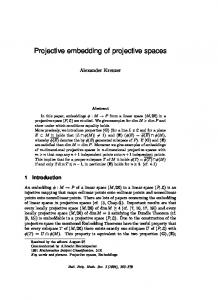
orientations of the polygons. One may assume in addition that the first vertex of the inscribed polygon is inside of the first side of the circumscribed one. The generator of the cyclic group shifts cyclically the order by one. b of One can unify these two moduli spaces by considering the moduli space T3 (S) framed convex projective structures on surfaces with geodesic boundary, equipped with a finite (possible empty) collection of marked points on the boundary, see Section 2.7. Our goal is to introduce a set of global coordinates on T3+ (S), describe its natural Poisson structure in terms of these parametrization and give explicit formulae for the maps i, µ, σ and the action of the mapping class group. Before addressing this problem, let us first solve this problem for the toy model P3n since it contains most of the tools used for the problem in question. 3. Parameterizations of the spaces P3n . Cut the inscribed polygons into triangles and mark two distinct points on every edge of the triangulation except the edges of the polygon. Mark also one point inside each triangle. Theorem 2.2 There exists a canonical bijective correspondence between the space P3n and assignments of positive real numbers to the marked points. Proof. It is constructive: we are going to describe how to construct numbers from a pair of polygons and visa versa. A small remark about notations. We denote points (resp. lines) by uppercase (resp. lowercase) letters. A triangle on RP2 is determined neither by vertices nor by sides, since there exists four triangles for any generic triple of vertices or sides. If the triangle is shown on a figure, it is clear which one corresponds to the vertices since only one of the four fits entirely into the drawing. If we want to indicate a triangle which does not fit, we add in braces a point which belongs to the interior of the triangle. For example, the points A, B and C on Figure 1 are vertices of the triangles ABC, ABC{a ∩ c}, ABC{a ∩ b} and ABC{b ∩ c}. Another convention concerns the cross-ratio. We assume that the cross-ratio of four points x1 , x2 , x3 , x4 on a line is the value at x4 of a projective coordinate taking value ∞ (x1 −x2 )(x3 −x4 ) at x1 , −1 at x2 , and 0 at x3 . So we employ the formula (x for the cross-ratio. 1 −x4 )(x2 −x3 ) Observe that the lines passing through a point form a projective line. So the cross-ratio of an ordered quadruple of lines passing through a point is defined. Let us first consider the case of P33 . It is the space of pairs of triangles abc and ABC (Figure 1), where the second is inscribed into the first and considered up to projective transformations. This space is one dimensional and its invariant X is just the cross-ratio of the quadruple of lines a, AB, A(b ∩ c), AC. Such invariant is called the triple ratio ([15], Section 3) and is defined for any generic triple of flags in RP2 and can be also defined as follows. Let R3 be the three dimensional real vector space whose projectivisation is RP2 . Choose linear functionals fa , fb , fc ∈ (R3 )∗ defining the lines a, b, c. Choose non-zero e B, e C e projecting onto the points A, B, C. Then vectors A, e b (C)f e c (A) e fa (B)f X := e b (A)f e c (B) e fa (C)f 5

b

C B

a c

A

Figure 1: P33 It is obviously independent on the choices involved in the definition, and manifestly Z/3Zinvariant. The third definition of the triple ratio is borrowed from ([16], Section 4.2). Every point (resp. line) of RP2 corresponds to a line (resp. plane) in V3 , and we shall denote them by the same letters. The line C belongs to the plane c and defines a linear map C : c∩a → c∩b: it is the graph of this map. Similarly there are linear maps A : a∩b → a∩c and B : b ∩ c → b ∩ a. The composition of these three linear maps is the multiplication by the invariant X. Elaborating the third definition using a Euclidean structure, we come to the fourth definition, making connection to the classical Ceva and Menelaus theorems: X := ±

|A(a ∩ b)||B(b ∩ c)||C(c ∩ a)| , |A(a ∩ c)||B(b ∩ a)||C(c ∩ b)|

where the distances are measured with respect to any Euclidean structure on R2 = RP2 − RP1 containing the triangles and the sign is positive if the triangles are inscribed on into another and minus otherwise. The Ceva theorem claims that the lines A(b ∩ c), B(c ∩ a) and C(a ∩ b) are concurrent (pass through one point) if and only if X = 1. The Menelaus theorem claims that the points A, B and C are concurrent (belong to a line) if and only if X = −1. In particular this definition implies the Lemma 2.3 X is positive if and only if ABC is inscribed into (a ∩ b)(b ∩ c)(c ∩ a). Now consider the next case: P34 . It is the space of pairs of quadrilaterals abcd and ABCD, where the second is inscribed into the first, considered up to projective transformations. The space of such configurations has dimension four. Two parameters of a configuration are given by the triple ratio X of the triangles ABC inscribed into abc and the triple ratio Y of ACD inscribed into acd{B} (Figure 2). Another two parameters are given by the cross-ratios of quadruples of lines a, AB, AC, AD and c, CD, CA, CB, denoted by Z and W , respectively. Assign the coordinates X, Y, Z and W to the marked points as shown on Figure 2. 6

b d C a

w y

D

x

B

z c A

Figure 2: P34 Lemma 2.4 The convex quadrangle ABCD is inscribed into the convex quadrangle abcd if and only if X, Y, Z, W are positive. Proof. Indeed, Lemma 2.3 implies that X, Y > 0. Observe that the cross-ratio of four points on RP1 is positive if and only if the cyclic order of the points is compatible with the one provided by their location on RP1 , i.e. with one of the two orientations of RP1 . This immediately implies that Z, W > 0. On the other hand, given X > 0 we have, by Lemma 2.3, a unique projective equivalence class of a triangle ABC inscribed into a triangle abc. We use the coordinates Z, W to define the lines AD and CD, and the positivity of Z and W guarantees that these lines intersect in a point D located inside of the triangle abc, that is in the same connected component as the triangle ABC. Finally, Y is used to define the line d, and positivity of Y just means that it does not intersect the interior of the quadrangle ABCD. The lemma is proved. Now let us consider the space P3n for an arbitrary n > 2. A point of this space is represented by a polygon A1 . . . An inscribed into a1 . . . an . Cut the polygon A1 . . . An into triangles. Each triangle Ai Aj Ak of the triangulation is inscribed into ai , aj ak , and we can assign their triple ratio to the marked point inside of Ai Aj Ak . Moreover for any pair of adjacent triangles Ai Aj Ak and Aj Ak Al forming a quadrilateral Ai Aj Ak Al inscribed into the quadrilateral ai aj ak al one can also compute a pair of cross-ratios and assign it to two points on the diagonal Aj Ak . The cross-ratio of the lines passing through Aj is associated to the point closer to the point Aj . The converse construction is straightforward. For every triangle of the triangulation one can construct a pair of triangles using the number in the center as a parameter and using Lemma 2.3. Then we assemble them together using numbers on edges as gluing parameters and Lemma 2.4. The theorem is proved. Now let us proceed to convex projective structures on surfaces.

7

4. A set of global coordinates on T3+ (S). Let S be a Riemann surface of genus g with s boundary components. Assume, that s ≥ 1 and moreover s ≥ 3 if g = 0. Shrink all boundary components to points. Then the surface S can be cut into triangles with vertices at the shrunk boundary components. We call it an ideal triangulation of S. Let us put two distinct marked points to each edge of the triangulation and one marked point to the center of every triangle. Theorem 2.5 Given an ideal triangulation T of S, there exists a canonical isomorphism {marked points} ∼ ϕT : T3 (S) −→ R>0 Proof. It is quite similar to the proof for P3n . Let us first construct a surface starting from a collection of positive real numbers on the triangulation. Consider the universal cover Se of the surface and lift the triangulation together with the marked points and numbers from S to it. According to Theorem 2.2 to any finite polygon composed of the triangles of the arising infinite triangulated polygon we can associate a pair of polygons in RP2 . Let U be the union of all inscribed polygons corresponding to such finite sub-polygons. Observe that it coincides with the intersection of all circumscribed polygons, and therefore is convex. The group π1 (S) acts on Se and hence on U by projective transformations. The desired projective surface is U/π1 (S). Now let us describe the inverse map, i.e. construct the numbers out of a given framed convex projective structure and a given triangulation. Take a triangle and send it to RP2 using a developing map ϕ. The vertices of the triangle correspond to boundary components. For a given boundary component Ci of S the choice of the developing map ϕ and the framing allows to assign a canonical flag (A, a) on RP2 invariant under the action of the monodromy operator around Ci . Indeed, if the boundary component Ci is non-degenerate, we take the line containing the interval ϕ(Ci ) for a, and one of the endpoints on this interval for A. The choice between the two endpoints is given by the framing, so that the interval is oriented out from the point A. If the boundary component is degenerate the point A is just the image of Ci under ϕ. The line a is the projectivization of the two-dimensional subspace where the monodromy operator µ(Ci ) acts by a unipotent transformation. Assigning the flags to all three vertices of the triangle one gets a point of P33 . The corresponding coordinate is associated to the central marked point of the original triangle. Similarly, taking two adjacent triangles of the triangulation one obtains the numbers for the marked points on edges. These two constructions are evidently mutually inverse to each other. The theorem is proved. 5. Properties of the constructed coordinates for both P33 and T3 (S). 1. It turns out that the Poisson brackets between the coordinates are very simple, namely {Xi , Xj } = 2εij Xi Xj , (1) 8

where εij is a skew-symmetric integral valued function. To define the function εij consider the graph with vertices in marked points and oriented edges connecting them as shown on Figure 3. (We have shown edges connecting marked points belonging to one triangle only. Points of other triangles are connected by arrows in the same way. Points connected by edges without arrows are not taken into account.) Then εij = (number of arrows from i to j) − (number of arrows from j to i) The proof of this formula amounts to a long computation. However it is an easy exercise to

Figure 3: Poisson structure tensor. verify that this bracket does not depend on the triangulation, and therefore can be taken just as a definition. For P3n it is the only natural way to define the Poisson structure known to us. 2. Once we have positive numbers assigned to marked points, the construction of the corresponding projective surface is explicit. In particular one can compute the monodromy group of the corresponding projective structure or, in other words, the image of the map µ. To describe the answer we use the following picture. Starting from the triangulation, construct a graph embedded into the surface by drawing small edges transversal to each side of the triangles and inside each triangle connect the ends of edges pairwise by three more edges, as shown on Figure 4. Orient the edges of the triangles in counterclockwise direction and the other edges in the arbitrary way. Let     0 0 1 0 0 Z −1 −1 −1  and E(Z, W ) =  0 −1 0  . T (X) =  0 X 1+X 1 W 0 0 Assign the matrix T (X) to the edges of each triangle with X assigned to its center. And assign the matrix E(Z, W ) to the edge connecting two triangles, where W (resp. Z) is the number to the left (resp. right) from this edge (Figure 4). Then for any closed path on the graph one can assign an element of P SL3 (R) by multiplying the group elements (or their inverses if the path goes along the edge against its orientation) assigned to edges the path passes along. The image of the fundamental group of the graph is just the desired monodromy group. The proof of this statement is also constructive. Once we have a configuration of flags from P33 with triple ratio X, one can define a projective coordinate system on RP2 . Namely, take the one where the point b ∩ c has coordinates [0 : 1 : 0]t , the point A has 9

. .

X

.

.

T(X)

T(X) E(Z,W)

.

.

.

. W

Z

.

T(X)

.

Y

.

T(Y)

.

T(Y) T(Y)

Figure 4: Construction of the monodromy group. coordinates [1 : −1 : 1]t , C – [1 : 0 : 0]t and B – [0 : 0 : 1]t (Figure 1). The line a has coordinates[1 : 1 + X : X]. The cyclic permutation of the flags induces the coordinate change given by the matrix T (X). Similarly if we have a quadruple of flags F1 F2 F3 F4 with two cross-ratios Z and W , then the coordinate system related to the triple F2 F4 F1 is obtained from the coordinate system related to the triple F4 F2 F3 by the coordinate change E(Z, W ) . Z(1+X) (1+Y ) and W ′ = X(1+Y : 3. The involution σ acts in a very simple way, where Z ′ = W Y (1+X) )

1/X

X W

Z

Z’

W’

Y

1/Y

Figure 5: Involution σ. In particular a point of T3 (S) is stable under σ if the two coordinates on each edge coincide, and the coordinates in the center of each triangle are equal to one. Taking into account that the set of σ-stable points is just the ordinary Teichm¨ uller space, one obtains its parametrisation. Actually it coincides with the one described in [5]. 4. Each triangulation of S provides its own coordinate system and in general the transition from one such system to another one is given by complicated rational maps. However any change of triangulation may be decomposed into a sequence of elementary changes — the so called flips. A flip removes an edge of the triangulation and inserts another one into the arising quadrilateral as shown on Figure 6. This figure shows also how the numbers at the marked points change under the flip. Observe that these formulae allow in particular to pass from one triangulation to the same one, but moved by a 10

nontrivial element of the mapping class group of S, and thus give explicit formulae for the mapping class group action. B A

D

X Z

A’

E

D’

W’ E’

Y’

H’

F

G

C’ X’

Z’

W Y

H

B’

C

G’

F’

Figure 6: Flip. Here A′ = A(1 + Z),

D′ = D

W , 1+W

E ′ = E(1 + W ),

H′ = H

Z , 1+Z

(1 + W )XZ 1 + Z + ZX + ZXW , C′ = C (1 + Z) 1 + Z + ZX + ZXW 1 + W + WY + WY Z (1 + Z)Y W F′ = F , G′ = G , (1 + W ) 1 + W + WY + WY Z 1+Z 1+W X′ = , Y′ = , XZ(1 + W ) Y W (1 + Z) 1 + W + WY + WY Z 1 + Z + ZX + ZXW Z′ = X , W′ = Y . 1 + Z + ZX + ZXW 1 + W + WY + WY Z The formulae can be derived directly, or more simply as in Section 11 in [6]. We will return to discussion of the structure of these formulas in Section 2.5 below. B′ = B

6. Convex projective structures on surfaces with piecewise geodesic boundary. A convex projective structure on a surface has piecewise geodesic boundary if a neighborhood of every boundary point is projectively isomorphic to a neighborhood of a boundary point of a half plane or a vertex of an angle. In the latter case it makes sense to consider a line passing through the vertex “outside” of the surface, see the punctured lines on Figure 7. Let us introduce framed convex projective structure with piecewise geodesic boundary. Let Sb be a pair consisting of an oriented surface S with the boundary ∂S, and a finite (possibly empty) collection of distinguished points {x1 , ..., xk } on the boundary. We define the punctured boundary of Sb by ∂ Sb := ∂S − {x1 , ..., xk }

So the connected components of ∂ Sb are either circles or arcs. 11

Definition 2.6 A framed convex projective structure with piecewise geodesic boundary on Sb is a convex projective structure on S with the following data at the boundary: i) Each connected component of the punctured boundary ∂ Sb is a geodesic interval. Moreover at each point xi we choose a line passing through xi outside of S, as on Figure 7. ii) If a boundary component does not contain distinguished points, we choose its orientation. b parametrises framed convex projective structures with piecewise geodesic The space T3 (S) b boundary on S. Remark. Sometimes it is useful to employ a different definition of the framing. Namely, instead of choosing lines through the distinguished points xi we choose a point b is pi inside of each of the geodesic segments bounded by the distinguished points. T3 (S) the moduli space of each of these two structures on S. Indeed, the equivalence between the two definitions is seen as follows. Consider the convex hull of the points pi . We get a surface S ′ inscribed into S, with the induced convex projective structure. Conversely, given S ′ we reconstruct S by taking the circumscribed surface.

S

Figure 7: Framed piecewise geodesic boundary of a convex projective structure on S The convexity implies that each boundary component develops into a convex infinite polygon connecting two points in RP2 , stabilized by the monodromy around the component. Moreover at each vertex of this polygon there is a line segment located outside of e S. b Indeed, Both spaces T3 (S) and P3n are particular cases of the moduli space T3 (S). n T3 (S) is obtained when the set {p1 , ..., pk } is empty, and we get P3 when S is a disc: in this case S is a convex polygon, serving as the inscribed polygon, and the circumscribed polygon is given by the chosen lines. To introduce the coordinates let us shrink the boundary components without marked points into punctures, and take a triangulation T of S with vertices at the distinguished points on the boundary and at the shred boundary components. We call it ideal triangulation. The interior of each side of such a triangulation is either inside of S, or at the boundary. We assign the coordinates to the centers of the triangles and pairs of marked points on the internal sides of the triangulations. Namely, going to the universal cover Se of S, we get a triangulation Te there. Then, by the very definition, for every vertex pe of the triangulation Te there is a flag given at pe. We use these flags just as above. b has the same features 1.-4. as T3 (S). The only thing deserving a The space T3 (S) b ֒→ T3 (S). b We define the comment is construction of a canonical embedding i : T2 (S) 12

b as the space of pairs (a complete hyperbolic metrics on S, a Teichm¨ uller space T2 (S) distinguished collection of points {x1 , ..., xk } located at the absolute of S). A point of the absolute of S can be thought of as a π1 (S)-orbit on the absolute of the hyperbolic plane which is at the infinity of an end of S. Thus going to the universal cover of S in the Klein model we get a finite collection of distinguished points at every arc of the absolute corresponding to an end of S. It remains to make, in a π1 (S)-equivariant way, finite geodesic polygons with vertices at these points, and add the tangent lines to the absolute at the vertices of these polygons. Taking the quotient by the action of π1 (S) we get a framed convex projective structure on S with piecewise geodesic boundary. 7. Comparing the moduli space of local systems and of convex projective structures. Let F be a set. Recall that an F -local system on a topological space X is a locally trivial bundle F on X, with fibers isomorphic to F and locally constant transition functions. If X is a manifold, this is the same thing as a bundle with a flat connection on X. If F is a group, we also assume that it acts on the right on F , and the fibers are principal homogeneous H-spaces. If G is an algebraic group, a G-local system on a variety X is an algebraic variety such that for a field K the set of its K-valued points is a G(K)-local system on X(K). Let G := P GL3 and let B be the corresponding flag variety. The set of its real points of was denoted by F3 above. For a G-local system L on S let LB := L ×G B be the associated local system of flags. Recall (Section 2 of [6]) that a framed G-local system on Sb is a pair (L, β) consisting of a G-local system on S and a flat section β of the restriction b The corresponding moduli space is denoted by of LB to the punctured boundary ∂ S. XG,Sb . Let us shrink all holes on S without distinguished points to punctures. An ideal triangulation T of Sb is a triangulation of S with vertices either at punctures or at the boundary components, so that each connected component of ∂ Sb hosts exactly one vertex of the triangulation. Repeating the construction of Sections 2.4-2.5 we get a set of coorb Precisely, given ideal dinate systems on XG,Sb parametrized by ideal triangulations of S. triangulations T there is an open embedding ϕT : G{minternal edges of T } ֒→ XG,Sb

Here Gm stays for the multiplicative group understood as an algebraic group. So the set of its complex points is C∗ . The natural coordinate on Gm provides a rational coordinate function on the moduli space XG,Sb . Thus the map ϕT provides a (rational) coordinate system on the moduli space. The transition functions between the two coordinate systems corresponding to triangulations related by a flip are given by the formulas written in the very end of Section 2.6. Since these formulas are subtraction free, the real locus of XG,Sb contains a well-defined subset   {internal edges of T } XG,Sb (R>0 ) := ϕT R>0 ֒→ XG,Sb (R) b Theorem 2.7 There is a canonical identification XP GL3 ,Sb (R>0 ) = T3 (S). 13

b is the subset of the real locus of the moduli space X In other words, T3 (S) P GL3 ,Sb consisting of the points which have positive real coordinates in the coordinate system corresponding b to one (and hence any) ideal triangulation of S. b parametrises the structures described in the Remark Proof. We will assume that T3 (S) after Definition 2.6. (If we adopt Definition 2.6, the distinguished points will play different roles in the definition of these moduli spaces). Let us define a canonical embedding b → X b (R>0 ). The local system Lp corresponding to a point p ∈ T3 (S) b is the one T3 (S) G,S corresponding to the representation µ(p). Intrinsically, it is the local system of projective frames on S. Let us define a framing on it. Let Ci be a boundary component of S. If it does not contain the distinguished points, the corresponding component of the framing is provided by the flag (a, A) defined in the proof of Theorem 2.5. If Ci contains distinguished points, we use the flag (p, L) where p is the chosen point on the boundary geodesic interval L. The restriction of the canonical coordinates on the moduli space XP GL3 ,Sb to the space of convex projective structures gives, by the very definition, the coordinates on the latter space defined above. Now the proof follows immediately from the results of Sections 2.3-2.5. The theorem is proved. 8. Laurent positivity properties of the monodromy representations. Consider the universal P GL3 -local system on the space S×XP GL3 ,S . Its fiber over S×p is isomorphic to the local system corresponding to the point p of the moduli space XP GL3 ,S . Our next goal is to study its monodromy representation. Let FS be the field of rational functions on the moduli space XP GL3 ,S . The monodromy of the universal local system around a loop on S is a conjugacy class in P GL3 (FS ). Recall that, given an ideal triangulation T of S, we defined canonical coordinates {XiT } on XP SL3 ,S corresponding to T . Given a coordinate system {Xi }, a positive rational function in {Xi } is a function which can be presented as a ratio of two polynomials in {Xi } with positive integral coefficients. For instance 1 − x + x2 is a positive rational function since it is equal to (1+x3 )/(1+x). A matrix is totally positive if all its minors are non-zero positive rational functions in {XiT }. Similarly we define upper/lower triangular totally positive matrices: any minor, which is not identically zero for generic matrix in question, is a positive rational functions. Theorem 2.8 Let T be an ideal triangulation of S. Then monodromy of the universal P GL3 -local system on S × XP GL3 ,S around any non-boundary loop on S is conjugate in P GL3 (FS ) to a totally positive matrix in the canonical coordinates assigned to T . The monodromy around a boundary component is conjugated to an upper/lower triangular totally positive matrix. Proof. Recall the trivalent graph Γ′T on Figure 4, defined starting from an ideal triangulation T of S. Let us call its edges forming the little triangles by t-edges, and the edges dual to the edges of the triangulation T by e-edges. The matrices T (∗) and E(∗) assigned in Section 5.2 to the t- and e-edges of this graph provide an explicit construction of the universal local system. Indeed, since T (X)3 is the identity in P GL3 , we get a universal local system on the dual graph to T . This graph is homotopy equivalent to S. 14

Given a loop on S, we shrink it to a loop on Γ′T . We may assume that this loop contains no consecutive t-edges: indeed, a composition of two t-edges is a t-edge. Thus we may choose an initial vertex on the loop so that the edges have the pattern et...etet. Therefore the monodromy is computed as a product of matrices of type ET or ET −1 . Observe that   −1 Z X Z −1 (1 + X) Z −1 1 1  and (2) E(Z, W )T (X) =  0 −1 0 0 W  Z −1 0 0  1 0 E(Z, W )T (X)−1 =  1 −1 −1 W W (1 + X ) W X 

.

(3)

These matrices are upper/lower triangular totally positive integral Laurent matrices in the coordinates X, Y, Z, W . A loop on S contains matrices of just one kind if and only if it is the loop around a boundary component. Therefore the monodromy around any nonboundary loop is obtained as a product of both lower and upper triangular matrices. It remains to use the following fact: if Mi is either lower or upper triangular totally positive matrix, and there are both upper and lower triangular matrices among M1 , ..., Mk , then the product M1 ...Mk is a totally positive matrix (cf. [11]). The theorem is proved. We say that the monodromy of a P GL3 (R)-local system is regular hyperbolic if the monodromy around a non-boundary loop has distinct real eigenvalues, and the monodromy around a boundary component is conjugated to a real totally positive upper triangular matrix. Corollary 2.9 The monodromy of a convex projective structure with geodesic boundary on S is faithful and regular hyperbolic. Proof. Follows immediately from Theorem 2.8 and the Gantmacher-Krein theorem [11] (see Chapter 2, Theorem 6 there) claiming that the eigenvalues of a totally positive matrix are distinct real numbers. The corollary is proved 1 Remark. Both Theorem 2.8 and Corollary 2.9 can be generalized to the case when G is an arbitrary split reductive group with trivial center, see [6]. When the boundary of S is empty and G = P SLm (R), a statement similar to Corollary 2.9 was proved in [21]. A Laurent polynomial in {XiT } is positive integral if its coefficients are positive integers. A rational function on the moduli space XP GL3 ,S is called a good positive Laurent polynomial if it is a positive integral Laurent polynomial in every canonical coordinate system on XP GL3 ,S . Corollary 2.10 The trace of the n-th power of the monodromy of the universal P GL3 local system on S around any loop on S is a good positive Laurent polynomial on XP GL3 ,S . 1

As was pointed out by the Referee, an alternative proof of Corollary 2.9 follows from the results of [13] for surfaces without boundary by doubling along the geodesic boundary.

15

Proof. A product of matrices with positive integral Laurent coefficients is again a matrix of this type. So the corollary follows from the explicit construction of the universal P GL3 -local system given in the proof of Theorem 2.8, and formulas (2)-(3). A good positive Laurent polynomial on XP GL3 ,S is indecomposable if it can not be presented as a sum of two non-zero good positive Laurent polynomials on XP GL3 ,S . Conjecture 2.11 The trace of the n-th power of the monodromy of the universal P GL3 local system on S around any loop on S is indecomposable.

3

The universal P SL3(R)-Teichm¨ uller space

In this Section, using the positive configuration of flags, we introduce the universal Teichm¨ uller space T3 for P SL3 (R). We show that the Thompson group acts by its automorphisms, preserving a natural Poisson structure on it. We show that T3 is closely related to the space of convex curves in RP2 . We leave to the reader to formalize a definition of a finite cyclic set. As a hint we want to mention that a subset of an oriented circle inherits a cyclic structure. 1. The universal higher Teichm¨ uller space. Definition 3.1 i) A set C is cyclically ordered if any finite subset of C is cyclically ordered, and any inclusion of finite subsets preserves the cyclic order. ii) A map β from a cyclically ordered set C to the flag variety F3 is positive if it maps every cyclically ordered quadruple (a, b, c, d) to a positive quadruple of flags (β(a), β(b), β(c), β(d)). A positive map is necessarily injective. So, abusing terminology, we define positive subset C ⊂ F3 as the image of a positive map, keeping in mind a cyclic structure on C. The set of positive n-tuples of flags in F3 is invariant under the operation of reversing the cyclic order to the opposite one. So it has not only cyclic, but also dihedral symmetry. Consider a cyclic order on P1 (Q) provided by the embedding P1 (Q) ֒→ P1 (R). Definition 3.2 The universal higher Teichm¨ uller space T3 is the quotient of the space of 1 positive maps β : P (Q) −→ F3 by the action of the group P SL3 (R). Canonical coordinates on T3 . Let us choose three distinct points on P1 (Q), called 0, 1, ∞. Recall the Farey triangulation, understood as a triangulation of the hyperbolic disc with a distinguished oriented edge. Then we have canonical identifications P1 (Q) = Q ∪ ∞ = {vertices of the Farey triangulation} The distinguished oriented edge goes from 0 to ∞. Consider the infinite set I3 := {pairs of points on each edge of the Farey triangulation}∪ {(centers of the) triangles of the Farey triangulation} 16

(4)

A point of T3 gives rise to a positive map {vertices of the Farey triangulation} −→ F3 considered up to the action of P GL3 (R). We assign to every triple of flags at the vertices of a Farey triangle their triple ratio, and to every quadruple of flags at the vertices of a Farey quadrilateral the related two cross-ratios, pictured at the diagonal. We get a canonical map I3 ϕ3 : T3 −→ R>0 (5) Theorem 3.3 The map (5) is an isomorphism. Proof. It is completely similar to the one of Theorem 2.2, and thus is omitted. The right hand side in (5) has a natural quadratic Poisson structure given by the formula (1). Using the isomorphism ϕ3 , we transform it to a Poisson structure on T3 . Here is another way to produce points of T3 . 2. Convex curves on RP2 and positive curves in the flag variety F3 . Let K be a continuous closed convex curve in RP2 . Then for every point p ∈ K there is a nonempty set of lines intersecting K at p and such that K is on one side of it. We call them osculating lines at p. A regular convex curve in RP2 is a continuous convex curve which has exactly one osculating line at each point. Assigning to a point p of a regular e in the flag convex curve K the unique osculating line at p we get the osculating curve K variety F3 . It is continuous. Moreover, thanks to the results of Section 2.3, it is positive, e ⊂ F3 is positive. It follows that K is a C 1 –smooth convex curve in i.e. the map K → K

Figure 8: Osculating lines to a convex curve. e is given by the flags (p, Tp K) where p runs through K. RP2 , and the osculating curve K It turns out that this construction gives all positive continuous curves in the flag variety F3 . Recall the double bundle p pb b2 RP2 ←− F3 −→ RP b2 is the set of lines in RP2 . A subset of RP2 is strictly convex if no line contains where RP its three distinct points. (warning: a strictly convex curve is a strictly convex subset, but a convex domain is never a strictly convex subset). Proposition 3.4 i) If C a positive subset of F3 , then p(C) and pb(C) are convex. ii) If C is a continuous positive curve in F3 , then p(C) is a regular convex curve. This gives rise to a bijective correspondence continuous positive curves in F3 regular convex curves in RP2 . 17

(6)

Proof. i) Follows immediately from the results of Section 2.3. ii) p(C) is continuous and, by i), convex. It comes equipped with a continuous family of osculating lines. It follows from this that p(C) is regular. This gives the arrow => in (6). The osculating curve provide the opposite arrow. Since a convex curve can not have two different continuous families of osculating lines, we got a bijection. The proposition is proved. So identifying P 1 (Q) with a subset of a regular convex curve K respecting the cyclic orders we produce a point of T3 . The Thompson group T. It is the group of all piecewise P SL2 (Z)-projective automorphisms of P1 (Q). By definition, for every g ∈ T there exists a decomposition of P1 (Q) into a union of finite number of segments, which may intersect only at the ends, so that the restriction of g to each segment is given by an element of P SL2 (Z). The Thompson group acts on T3 in an obvious way. Here is another way to look at it. The Thompson group contains the following elements, called flips: Given an edge E of a triangulation T with a distinguished oriented edge, we do a flip at E (as on the Figure 6), obtaining a new triangulation T ′ with a distinguished oriented edge. Observe that the sets of ends of the trivalent trees dual to the triangulations T and T ′ are identified. On the other hand, there exists unique isomorphism of the plane trees T and T ′ which identifies their distinguished oriented edges. It provides a map of the ends of these trees, and hence an automorphism of P 1 (Q), which is easily seen to be piecewise linear. The Thompson group is generated by flips ([18]). So the formulas in the end of Section 2.5 allow to write the action of the Thompson group explicitly in our coordinates. Proposition 3.5 The action of the Thompson group preserves the Poisson bracket on T3 . Proof. Each flip preserves the Poisson bracket. The proposition follows. Let H be the hyperbolic plane. For a torsion free subgroup ∆ ⊂ P SL2 (Z), set S∆ := H/∆. Proposition 3.6 The Teichm¨ uller space T3 (S∆ ) is embedded into the universal Teichm¨ uller space T3 as the subspace of ∆-invariants: T3 (S∆ ) = (T3 )∆

(7)

This isomorphism respects the Poisson brackets. Demonstration. The surface S∆ has a natural triangulation T∆ , the image of the Farey triangulation under the projection π∆ : H → S∆ . So according to Theorem 2.2 the left hand side in (7) is identified with the positive valued functions on I3 /∆, that is with ∆-invariant positive valued functions on I3 . It remains to use Theorem 3.3. The claim about the Poisson structures follows from the very definitions. The proposition is proved. Remark 1. The mapping class group of S∆ is not embedded into the Thompson group, unless we want to replace the latter by a bigger group. Indeed, a flip at an edge 18

E on the surface S∆ should correspond to the infinite composition of flips at the edges of the Farey triangulations projected onto E. Nevertheless the Thompson group plays the role of the mapping class group for the universal Teichm¨ uller space. Remark 2. The analogy between the mapping class groups of surfaces and the Thompson group can be made precise as follows. In Chapter 2 of [7] we defined the notion of a cluster X -space (we recall it in the Section 4.3), and the mapping class group of a cluster X -space, acting by automorphisms of the cluster X -space. The classical and the universal Teichm¨ uller spaces can be obtained as the spaces of R>0 -points of certain cluster X -spaces, which were defined in [6]. The corresponding mapping class groups are the classical mapping class groups, and the Thompson group, see Sections 2.9 and 2.14 in [7] for more details. Remark 3. The universal Teichm¨ uller space and the SL3 Gelfand-Dikii Poisson brackets. The functional space of osculating curves to smooth curves has a natural Poisson structure, the SL3 Gelfand-Dikii bracket. One can show that its restriction to the subspace provided by the regular convex curves is compatible with our Poisson bracket.

4

The quantum P GL3-Teichm¨ uller spaces

In this Section we introduce the quantum universal P GL3 -Teichm¨ uller space. We proved that the Thompson group acts by its automorphisms. In particular this immediately gives a definition of the quantum higher Teichm¨ uller space of a punctured surface S, plus the fact that the mapping class group of S acts by its automorphisms. 1. The quantum torus related to the set I3 . Let T3q be a non-commutative algebra, (a quantum torus), generated by the elements Xi , where i ∈ I3 , subject to the relations q −εij Xi Xj = q −εji Xj Xi , i, j ∈ I3 (8) Here q is a formal variable, so it is an algebra over Z[q, q −1 ]. The algebra T3q is equipped with an antiautomorphism ∗, acting on the generators by ∗(Xi ) = Xi ,

∗(q) = q −1

(9)

Let us denote by Frac(T3q ) its non-commutative fraction field. 2. The Thompson group action: the quasiclassical limit. Recall that the Thompson group T is generated by flips at edges of the Farey triangulation. Given such an edge E, let us define an automorphism ϕE : Frac(T3 ) −→ Frac(T3 )

where T3 := T31

Consider the 4-gon of the Farey triangulation obtained by gluing the two triangles sharing the edge E — see Figure 6, where E is the horizontal edge. Let SE ⊂ I3 be the 12-element

19

set formed by the pairs of marked points on the four sides and two diagonals of the 4-gon. On Figure 6 these are the points labeled by A, B, ..., Z, W . We set  ′ Xi i ∈ S E ϕE (Xi ) := Xi i 6∈ SE where Xi′ is computed using the formulas after Figure 6, so for instance if Xi = A, then Xi′ = A′ and so on. Proposition 4.1 The automorphisms ϕE give rise to an action of the Thompson group T by automorphisms of the field Frac(T3 ) preserving the Poisson bracket. Proof. It is known that the only relations between the flips fE are the following ones: i)fE2 = Id,

ii)fE1 fE2 = fE2 fE1 if E1 and E2 are disjoint,

iii)(fE5 fE4 fE3 fE2 fE1 )2 = Id

where the sequence of flips fE1 , ..., fE5 is shown on Figure 9. The first two relations

Figure 9: Pentagon relation. are obviously valid. The pentagon relation iii) is clear from the geometric origin of the formula. The proposition is proved. To introduce the action of the Thompson group on the non-commutative field Frac(T3q ), let us recall some facts about the quantum cluster ensembles from [7]. 3. The cluster X -space and its quantization. The cluster X -space is defined by using the same set-up as the cluster algebras [9]. We start from the quasiclassical case. Consider the following data I = (I, ε), called a seed: i) A set I, possibly infinite. ii) A skew-symmetric function ε = εij : I × I → Z. We assume that for every i ∈ I, the set of j’s such that εij 6= 0 is finite. A mutation in the direction k ∈ I changes the seed I to a new one I′ = (I, ε′ ) where the function ε′ is given by the following somewhat mysterious formula, which appeared in [9] in the definition of cluster algebra:  −εij if k ∈ {i, j} ′ εij = (10) εij + εik max{0, sgn(εik )εkj } if k 6∈ {i, j} A seed may have an automorphism given by a bijection I → I preserving the ε-function. A cluster transformation is a composition of mutations and automorphisms of seeds. 20

We assign to a seed I a Poisson algebra TI := Q[Xi , Xi−1 ], i ∈ I with the Poisson bracket {Xi , Xj } = εij Xi Xj Observe that the algebra TI is the algebra of regular functions on an algebraic tori XI : for any field K, the set of its K-valued points is (K ∗ )I . Let us take another seed I′ = (I, ε′ ) with the same set I, and consider a homomorphism µk : Frac(TI′ ) −→ Frac(TI ) defined on the generators by  if k 6= i, εik ≤ 0  Xi (1 + Xk )−εik −1 −εik ′ Xi (1 + Xk ) if εik > 0 µk (Xi ) := (11)  −1 Xk if k = i The following result could serve as a motivation for the formula (10)

Lemma 4.2 The map µk preserves the Poisson bracket if and only if the functions ε′ij and εij are related by the formula (10) Proof. Straightforward. The cluster X -space is a (11). It can be understood corresponding to all seeds J according to these birational

geometric object describing the birational transformations as a space X|I| obtained by gluing the algebraic tori XJ , obtained from the initial one I by cluster transformations, transformations.

Now let us turn to the quantum case. Given a seed, consider the non-commutative fractions field Frac(TIq ) of the algebra generated by the elements Xi , i ∈ I, subject to the relations (8). It is a non-commutative ∗-algebra, with an automorphism ∗ given by (9). It was proved in Section 3 of [7] that there is a ∗-algebra homomorphism µk : Frac(TIq′ ) −→ Frac(TIq ) acting on the generators by

where

  Xi G|εik | (q; Xk ) Xi G|ε | (q; Xk−1)−1 µk (Xi ) =  −1 ik Xk Ga (q; X) :=

 Qa

i=1 (1

1

if k 6= i, εik ≤ 0 if εik > 0 if k = i

+ q 2i−1 X) a > 0 a=0

4. The main result. Our goal is the following theorem. Theorem 4.3 The Thompson group T acts by ∗-automorphisms of the non-commutative field Frac(T3q ), so that specializing q = 1 we recover the action from Proposition 4.1. 21

Proof. To get the explicit formulae for the action of flips, we will apply the above construction to the situation when I = I3 , and the function εij was defined in Section 2.5. We define a flip ϕE : Frac(T3q ) −→ Frac(T3q ) as the composition of the mutations in the directions of Z, W, X, Y on Figure 6. An easy computation, presented in the subsection 4.6 in the quantum form, shows that in the case q = 1 this leads to the formulas after Figure 6. In the general case one needs to check the relations for the flips. The first two of them are obvious. The quantum pentagon relation can be checked by a tedious computation, using the explicit formulas for the quantum flip given in the subsection 4.6. Observe that fE5 fE4 fE3 fE2 fE1 differs from the identity only by an involution of the seven variables assigned to the marked points inside of the pentagon. The theorem is proved. The universal P GL3 -Teichm¨ uller space story from this point of view looks as follows: Theorem 4.4 The universal Teichm¨ uller space T3 is the set of the positive real points of the cluster X -space related to the seed {the set I3 , the cluster function εij defined in Section 2.5} The Thompson group is a subgroup of the mapping class group of the corresponding cluster ensemble. Remark. The quantum universal higher Teichm¨ uller space and the W3 -algebra. We suggest that the action of the Thompson group by birational ∗-automorphisms of the quantum universal Teichm¨ uller space T3q should be considered as an incarnation of the W -algebra corresponding to SL3 . (For a down-to-earth definition of W3 -algebras see [2]; for an algebraic-geometric discussion of W -algebras see [1]). 5. The quantum P GL3 -Teichm¨ uller space for a punctured surface. Let us present a punctured surface S as S = S∆ := H/∆, where ∆ is a subgroup of P SL2 (Z), as in Section 3.2. Definition 4.5 The quantum higher Teichm¨ uller space X3q (S∆ ) for a punctured surface S∆ is given by (12) X3q (S∆ ) := Frac(T3q )∆ Theorem 4.3 immediately implies Corollary 4.6 The mapping class group of S acts by positive birational ∗-automorphisms of the ∗-algebra (12).

22

6. Appendix: Formulas for a quantum flip. Performing mutations at Z and W we get B1 = B, C1 = C, F1 = F, G1 = G, Z1 = Z −1 , W1 = W −1 A1 = A(1 + qZ),

D1 = D(1 + qW −1)−1 ,

H1 = H(1 + qZ −1 )−1 ,

X1 = X(1 + qZ −1 )−1 (1 + qW ),

E1 = E(1 + qW ),

Y1 = Y (1 + qZ)(1 + qW −1 )−1

Mutations of the ε-function are illustrated on Figure 10, where the centers of mutations

mutations at

mutations at

X 1 and Y 1

Z and W

Figure 10: Mutations of the ε-function are shown by little circles. Performing mutations at X1 and Y1 we arrive at the final formulas for the quantum flip: A′ = A(1 + qZ),

D ′ = D(1 + qW −1 )−1 ,

E ′ = E(1 + qW ),

X ′ = (1 + qW )−1(1 + qZ −1 )X −1 ,

H ′ = H(1 + qZ −1 )−1 ,

Y ′ = (1 + qW −1 )(1 + qZ)−1 Y −1 ,

B ′ = B(1 + qZ)−1 (1 + qZ + q 2 ZX + q 3 ZXW ) F ′ = F (1 + qW )−1 (1 + qW + q 2 W Y + q 3 W Y Z)  −1 C ′ = CZX(1 + qW ) 1 + q −1 Z + q −2 XZ + q −3 W XZ

G′ = GW Y (1 + qZ)(1 + q −1 W + q −2 Y W + q −3 ZY W )−1  −1 Z ′ = X(1+qW ) 1+q −1Z +q −2 XZ +q −3W XZ (1+qW )−1(1+qW +q 2W Y +q 3 W Y Z)  −1 W ′ = W −1 (1+qZ)−1(1+qZ+q 2 ZX+q 3ZXW )W Y (1+qZ) 1+q −1 W +q −2 Y W +q −3 ZY W

23

5

Appendix: the configuration space of 5 flags in P2 is of cluster type E7.

If mutating the X-coordinates (as in (11)) we get only a finite collection of different coordinate systems, we say that the corresponding cluster X -space is of finite type. Based on the Fomin-Zelevinsky classification theorem [10], we showed in [7] that cluster X -spaces of finite type are also parametrised by Dynkin diagrams of the Cartan-Killing type. In this paper, we defined cluster X -spaces under a simplifying assumption that the matrix εij is skew-symmetric. In the finite type case this boils down to the condition that the Dynkin diagram is simply-laced. Every skew-symmetric matrix ε : J × J → Z with integer entries determines a graph with oriented edges. Namely take J as the set of vertices and connect vertices i and j by |εij | edges oriented towards j if εij > 0 and towards i otherwise. Conversely any graph with oriented edges and such that edges connecting any two vertices have the same orientation we can associate a skew-symmetric matrix. Graph notation for skew symmetric matrices is sometimes more convenient than the matrix notation. Below we use this to picture a function εij from a seed I = (I, ε) by an oriented graph. A mutation is determined by a vertex k, pictured by a little circle around the vertex. The mutated function ε′ij is given by formula (10). If εkl = 0, the mutations at the vertices k, l commute, so we may picture both of them on the same diagram. The mutated graph is shown on the right of the initial one. Finally, a seed I = (I, ε) is of finite type if mutating the graph of ε we can get a graph isomorphic to the Dynkin diagram of type An , Dn , E6 , E7 , E8 , oriented in a certain way.

Figure 11: The moduli space of configurations of 4 flags in P GL3 is of cluster type D4 . Proposition 5.1 a) The moduli space of configurations of 4 flags in P GL3 has a structure of a cluster X -space of finite type D4 . b). The moduli space of configurations of 5 flags in P GL3 has a structure of a cluster X -space of finite type E7 . Proof. We exhibit a sequence of mutations of the ε-function transforming the εfunction describing the moduli space of configurations of 4 (respectively 5) flags in P GL3 to a standard one of finite type D4 (respectively E7 ). The case n = 4 is shown on Figure ??, and the n = 5 case on Figure 12. The proposition is proved. Acknowledgments. This work has been done when V.F. visited Brown University. He would like to thank Brown University for hospitality and support. He wish to thank 24

Figure 12: Mutations leading to a standard ε-function of type E7 . grants RFBR 01-01-00549, 0302-17554 and NSh 1999.2003.2. A.G. was supported by the NSF grants DMS-0099390 and DMS-0400449. The paper was finished when A.G. enjoyed the hospitality of the MPI (Bonn). He is grateful to NSF and MPI for the support. We are very grateful to the Referee for many useful comments incorporated in the paper.

References [1] Beilinson A.A., Drinfeld V.G. Chiral algebras. AMS, Colloquium Publications, Volume 51, 2004. [2] A.A.Belavin: Equations of KdV type and W -algebras. Advanced Studies in Pure Mathematics. Integrable systems in Quantum Field Theory and Statistical Mechanics. 19 (1989), 117-125. [3] L.O.Chekhov, V.V.Fock: Quantum Teichm¨ uller spaces. Teoret. Mat. Fiz. 120 (1999), no. 3, 511–528. [4] S.Choi, W.Goldman: Deformation space of convex RP2 structures on 2-orbifolds. American Journal of Mathematics, vol. 127, no. 5, October 2005, pp. 1019-1102. [5] V.V.Fock, Dual Teichm¨ uller spaces. dg-ga/9702018. [6] V.V.Fock, A.B.Goncharov: Moduli spaces of local systems and higher Teichm¨ uller theory, math/0311149 [7] V.V.Fock, A.B.Goncharov: Cluster ensembles, quantization and the dilogarithm, math/0311245. [8] V.V.Fock, A.A.Rosly: Poisson structure on moduli of flat connections on Riemann surfaces and the r-matrix. AMS Transl. Ser. 2, 191, 67–86, 1999. 25

[9] Fomin S., Zelevinsky A.: Cluster algebras. I: Foundations. J. Amer. Math. Soc. 15 (2002), no. 2, 497–529. [10] Fomin S., Zelevinsky A.: Cluster algebras. II: Finite type classification. Invent. Math. 154 (2003), no. 1, 63–121. [11] F.P. Gantmacher, M.G. Krein: Oscillation matrices and kernels and small vibrations of mechanical systems. Revised edition of the 1941 Russian original. AMS Chelsea Publ., Providence, RI, 2002. [12] M.Gekhtman, M.Shapiro, A.Vainshtein: Cluster algebras and Poisson geometry. QA/0208033. [13] W.Goldman: Convex real projective structures on surfaces, J. Diff. G., 1990, 31, 795-845. [14] W.Goldman: Symplectic nature of fundamental groups of surfaces. Adv. in Math., Vol 54 (1984), 200-225. [15] A.B. Goncharov: Polylogarithms and motivic galois groups, Motives (Seattle, WA, 1991), 43–96, Proc. Sympos. Pure Math., 55, Part 2, Amer. Math. Soc., Providence, RI, 1994. [16] A.B. Goncharov: Polylogarithms, regulators and Arakelov motivic complexes, JAMS, vol 14, N1, (2005). 1-60. ArXive math.AG/0207036. [17] N.J.Hitchin: Lie groups and Teichmuller space. Topology 31 (1992)3, 449–473. [18] M. Imbert: Sur l’isomorphism du group de Richard Thompson avec le groupe de Ptol´em´ee. London Math. Soc. Lect. Note Ser., 243, Cambridge Univ. Press, 1997, 313-324. [19] Hong Chan Kim: The symplectic global coordinates on the moduli space of convex projective structures. J. Diff. Geom. 53 (1999), 359-401. [20] F.Labourie: RP2 -structures et differentielles cubiques holomorphes, Proc. of the GARC Conf. on Diff. Geom., Seoul Nat. Univ., 1997. [21] F.Labourie: Anosov flows, Surface Groups and Curves in Projective Space. math.DG/0401230. [22] J. Loftin: Affine structures and convex RP2 -manifolds, Am. J. Math., 123, 255-274, 2001. [23] R. Penner: Universal constructions in Teichm¨ uller theory. Adv. Math. 98 (1993), no. 2, 143–215.

26

[24] R. Penner: The universal Ptolemy group and its completions. Geometric Galois actions, 2, 293–312, London Math. Soc. Lect. Note Ser., 243, Cambridge Univ. Press, 1997.

27