Mathematical background for diffusion processes

Mathematical background for diffusion processes in natural porous media

Nicolae Suciu 1

Forschungszentrum J¨ ulich/ICG-4 Internal Report No. 501800 September 2000 Institut f¨ ur Erdöl und Organische Geochemie (ICG-4) Forschungszentrum J¨ ulich GmbH 52425 J¨ ulich Tel: 02461/61-4702 Telefax: 02461/61-2484 1

”Tiberiu Popoviciu” Institute of Numaerical Analysis, Cluj Napoca Branch of Romanian Academy

Forword This report contains the English abstract of the Ph.D. thesis, ”On the Connection Between the Microscopic and Macroscopic Modeling of the Thermodynamic Processes”, that the author defended at ”Simion Stoilow Institute of Mathematics of the Romanian Academy” in December 1998. Passing through general definitions and results from the mathematics of stochastic processes and dynamical systems as tools in nonequilibrium statistical mechanics (Section 2), this work presents a mathematical frame of ”stochastic theories” of diffusion in hydrogeological environments and proposes new approaches for both continuousmathematical and numerical modeling. The general frame allowing to obtain the connection between Lagrangian and Eulerian descriptions, to introduce Corsin’s conjecture and to discuss about asymptotic diffusive behavior is presented in Section 3. One underlines the difference between the genuine diffusion coefficients (3.4) and the effective ones (3.5), the requirement that more than one statistical ensemble should be defined to describe movements in random fields (two in (3.10) and three in (3.13), when both random field and local diffusion are considered) and the non-additivity between the ”molecular diffusion” and effective diffusion in absence of molecular diffusion (3.14-15). The continuous modeling based on space-time coarse grained averages from Section 4 outlines the derivation of Darcy-Buckingham law (4.15) and porosity dependent advectiondiffusion equation (4.16). This continuous modeling is also useful in designing random walkers numerical models for diffusion. The numerical models presented in Section 5 were tested for 1-dimensional diffusion at very small concentrations and model-problem of non-diffusive behavior in stratified aquifers of Matheron and de Marsily. These preliminary results are the basis of a numerical model for diffusion which is being developed in our research group. This short excursion through the field of irreversibility, continuous modeling and diffusion in random environments is based on the results from the author’s work during several stays in the research team ”Verhalten von Schadstoffen in geologischen systemen” at Forschungszentrum J¨ ulich. The references list of the report contains their previous results and relevant works for a thorough study of these problems.

J¨ ulich, September 5, 2000

Dr. H. Vereecken

”SIMION STOILOW” INSTITUTE OF MATHEMATICS OF THE ROMANIAN ACADEMY

NICOLAE SUCIU

ON THE CONNECTION BETWEEN THE MICROSCOPIC AND MACROSCOPIC MODELING OF THE THERMODYNAMIC PROCESSES

(The English abstract of the Ph.D. Thesis)

Scientific supervisor: Professor Dr. Adelina Georgescu Bucure¸sti, 1998

1

Introduction

The goal of statistical mechanics is to derive macroscopic behavior of physical systems from the behavior of their microscopic components [B˘alescu, 1975, pp.3, 34]. The specific paradigm is to study not a single physical system but large collections of identical systems, continuously distributed into the ’phases space’, called statistical ensemble. This is done by means of a density defined on the space of all possible states. It has the meaning of the probability density for the state of the system to correspond to a given point in the state space. The basic postulate of statistical mechanics [B˘alescu, 1975, p.724] says that the probability density provides a complete description of the system and statistical averages give macroscopic observable values of all physical quantities. In passing from a microscopic description, by dynamical systems, to a statistical macroscopic one, the ergodicity problem occurs: time and statistical averages must be equal in order to have the same observable value of the physical quantity in both descriptions. Moreover, if the statistical description uses the framework of state space then it is isomorphic to the deterministic description [Onicescu, 1977, p.363, Prigogine, 1998]. In this case the irreversible behavior, as described by increasing entropy, cannot be derived [Lasota and Mackey, 1994]. This is referred to as the Statistical mechanics paradox. These difficulties can be removed if the microscopic description uses the framework of stochastic processes, defined by probability measures on the space of trajectories of the microscopic constituents [Doob, 1953, chap.2]. The nondegenerate case is that one when through a given point passes a whole set of trajectories, and not only one trajectory as it is the case of dynamical systems. Stochastic processes also could be mathematical models for statistical ensemble of Gibbs and Boltzmann, ”a concept consisting of many physical systems with different initial conditions” [Boltzmann, 1981, p.204]. The probabilities on the state space are obtained by projections of probabilities defined on the space of trajectories. There exists a nontrivial class of Markov processes (including diffusion processes) which are ergodic and allow the derivation of the entropy law. In this general approach micoscopic dynamics does not explicitly occur. As a consequence, no ’correspondence principle’ can be used (for instance, one cannot find the Newtonian mechanics as a limiting case). The attempt of the ’Bruxelles school’ [Misra et al., 1979, Prigogine, 1980, 1999] to obtain ”a probabilistic reformulation of microscopic dynamics” yields representations of irreversible Markov processes by dynamical systems into measure spaces. But this abstract dynamics is not explicit, no equations of motion of physical particles are proposed, and correspondence principle is not yet established. This could be a reason for the dominant pragmatic attitude based on the remark that for many particle systems or for systems with sensible dependence on initial conditions deterministic predictions are inoperative. ”A paradigmatic jump” or ”a change of philosophy by supply of new concepts and probabilistic predictions” is claimed [Lebowitz, 1999, Parisi, 1999, Ruelle, 1999]. Despite of its foundation difficulties, statistical mechanics successfully solved many practical problems by using supplementary hypotheses. Among them, the thermodynamics of systems close to equilibrium gives good predictions for transport coefficients by Green-Kubo formulas and fluctuation-dissipation theorems [B˘alescu, 1975]. In order to achieve these, the microscopic description is proposed by Langevin type equations (generalizing Newton law up to a perturbed dynamical system). The corresponding continuous description is obtained as Fokker-Planck equations for probability densities. A frequently used complementary approach is the numerical procedure called the ’molecular dynamics’. According to this, the 1

behavior of physical systems is obtained through the simulation of the movement of a large number of particles followed by space-time averages yielding a continuous description [Koplik and Banavar, 1995]. * *

*

The Ph.D. thesis discusses a few questions on theoretical foundation of statistical mechanics, argues for a new method in continuous modeling of corpuscular physical systems and proposes a molecular dynamics type numerical approach for diffusion processes. ♦ Section 2 contains a general presentation of both stochastic processes and measure dynamical systems as random functions in the Doob sense. Deterministic processes are shown to be degenerated Markov processes. It is found that the ’strongly ergodic’ Markov processes, as defined by Gardiner [1983], describe irreversible thermodynamic behavior. Their representation as measure dynamical systems in spaces of trajectories could reformulate the Misra-Prigogine-Courbage theory of irreversibility. ♦ In the Section 3 diffusion processes are defined and equivalence between Fokker-Planck and Langevin equations is presented. Starting with the Langevin-like equation for the molecules motion, the Gibbs thermodynamic relation between free energy, entropy and temperature is derived. The transport coefficients are obtained as Green-Kubo formulas. Some definitions and results from the theory of diffusion in random fields are formulated and used to model turbulent diffusion and transport processes in porous media. ♦ Section 4 proposes a new macroscopic continuous model for discrete systems, based on [Vamo¸s et al., 1996a,b]. If physical quantities associated with particles can be described by piece-wise analytical functions then, coarse grained space-time averages give a.e. continuous fields verifying identities similar to balance equations from mechanics of continua. Throughout continuous fields and macroscopic balance equations are obtained by averaging over the statistical ensemble. The correspondence with classical results of Kirkwood [1967] is obtained for small space-time scales. In addition, it is shown that from the requirement that the concentration balance be a diffusion-like equation, a microscopic criterion for irreversibility is obtained. This could be useful in numerical simulations and experimental data analysis. As an illustration, a continuous model of transport processes in porous media, the derivation of Darcy law and porosity dependent transport equations are presented. ♦ On the basis of the results from the Section 4, the Section 5 develops a molecular dynamics type numerical model for diffusion. Continuous fields are derived by coarse grained averages over the trajectories of a system of random walkers evolving in a grid. The spacetime scale and the number of particles needed for a given precision is obtained, numerical and analytical solutions are compared and the microscopic irreversibility criterion is tested. Moreover, a two-dimension simulation of diffusion in a random field is performed to test the method by comparing its results with the features of the model of Matheron and de Marsily [1980].

2

Dynamical Systems and Stochastic Processes

Statistical mechanics description for a physical system consisting of N particles is given by systems of ordinary differential equations (Newton law or Hamiltonian system) dy (2.1) = V (y), y ∈ Y, Y ⊆ R6N , V ∈C 1 (Y ), dt 2

If there is a unique solution of the Cauchy problem (2.1), y(0) = y0 , for ∀ t ∈ R, then St (y0 ) = y(t, y0 ) defines a differentiable dynamical system, {St }t∈R , generated by the vectors field V . Moreover, the dynamical system preserves the Lebesgue measure, µ, defined on the Borel σ-algebra B, i.e. µ(B) = µ(S−t B), ∀ B ∈ B. It follows that {St }t∈R is a group of automorphisms in the measure space (Y, B, µ) (state space). Then, with the microscopic description (2.1) one associates the continuous macroscopic description given by the Frobenius-Perron unitary group [Cornfeld et al., 1982, pp.26,48], {Ut }t∈R , Ut : L1 (Y ) −→ L1 (Y ), (Ut f )(y) = f (S−t (y)).

(2.2)

Let p0 be the density of the measure P, absolutely continuous with respect to µ, P (B) = p (y)dy, ∀ B ∈ B. The evolution of p(y, t) = Ut p0 (y) is described by the Liouville equation, B 0 ∂p ∂ (pVk ) = 0. + ∂t k=1 ∂yk 6N

(2.3)

The projection of p on R3 is a concentration and from (2.3) one derives the continuity equation. Densities described by (2.2-3) conserve the Gibbs entropy S(t) = − p(y, t) ln p(y, t)dy = const. Thus, differentiable dynamical systems preserving a measure in the state space cannot be used as models for thermodynamic irreversibility [Gardiner, 1983, pp.61-62, Lasota and Mackey, 1994, chap.9]. Let Λ ⊆ R be a set of parameters, (Ω, A, P ) be a measure space with probability measure and let (Y, B) be a measurable space A. stochastic process is defined as a random variable η : Ω −→ Y Λ , η(ω) = y ω , y ω ∈ Y Λ , ∀ ω ∈ Ω.

(2.4)

The function y ω : Λ −→ Y, is a trajectory and its values, y ω (λ) = yλ , are points in the state space Y. If BΛ is a σ-algebra in Y Λ , then Pη (C) = P ({η ∈ C}), ∀C ∈ BΛ , define the distribution of the process (2.4) and the space of trajectories becomes a probability space, (Y Λ , BΛ , Pη ), called phase space. Uniquely up to an isomorphism, phase space defines the stochastic process in the sense of Doob. [Doob, 1953, Iosifescu and T˘autu, 1973]. When the microscopic description is performed by means of stationary Markov processes (i.e. the state after a time interval τ does not depend on the previous states), the continuous description can be obtained using semigroups of kernel type Markov operators, {Kτ }τ ≥0 , defined by (2.5) Kτ f (y) = p(y, τ | y0 )f (y0 )dy0 , ∀ f ∈ L1 (Y ), Y

where p(. | .) is the density of transition probability. The existence of the limit p(y1 , t1 − t2 | y2 ) −→ ps (y1 ), for t1 − t2 −→ ∞,

(2.6)

ensure the strong ergodicity [Gardiner, 1983, Sect.3.7.3]. With a strongly ergodic process one associates a non-stationary process through the ’preparation of an initial state’ [Gardiner, 1983, p.60, van Kampen, 1981, p.92] p(y, t) = p(y, t − t0 | y0 ) and p(y, t | y , t ) = p(y, t − t | y ), ∀ t, t > t0 , 3

(2.7)

for fixed t0 . These processes are also referred to as homogeneous processes. Their important property is the existence of the limit p(y, t) → ps (y) as t → ∞ (or t0 → −∞), which, when used in (2.5), implies (2.8) Kt p − ps L1 → 0, for t → ∞. The semigroups endowed with the property (2.8) are just the ’strong Markov’ [Misra et al., 1979] or ’irreversible’ [Antoniou and Gustafson, 1993] semigoups. For these semigroups the Gibbs entropy (and any convex functional of p) monotonically increases up to a maximum value corresponding to the equilibrium state, i.e. they satisfy the second law of thermodynamics. From (2.2) and (2.5) it follows that the Frobenius-Perron operators are Markov operators with a singular transition probability (between states lying on the same trajectory): p(y, t | y0 ) = δ(y − St (y0 )). This is the reason the dynamical systems are presented as degenerated Markov processes [Misra et al., 1979]. The following proposition was proved. Proposition 2.3: If the dynamical system {St }t∈R preserves a measure P in the states space, P (B) = P (S−t B), ∀ B ∈ B, then it generates a stochastic process in the sense of Doob, η, and the corresponding state and phase spaces are isomorphic: (Y, B, P ) ∼ (Y R , BR , Pη ). A stationary Markov process can be represented as a dynamical system in the space of its trajectories. By the Kolmogorov theorem [Iosifescu and T˘autu, 1973], the measure Pη is completely defined by the measure of the cylindrical sets from B R , defined as Cn+1 = {y ω (t0 ) ∈ B0 , · · · , y ω (tn ) ∈ Bn | B0 , · · · , Bn ∈ B}, t0 < · · · < tn . For Markov processes this reads Pη (Cn+1 ) = p(y0 , t0 )dy0 p(y1 , t1 | y0 , t0 )dy1 · · · p(yn , tn | yn−1 , tn−1 )dyn , B0

B1

B1

and the because the process is stationary, Pη (Cn+1 ) = Pη (Στ (Cn+1 )) = Pη (Σ−τ (Cn+1 )). The invertible map Στ : Y R −→ Y R , Στ (yt ) = yt+τ , (translation along the trajectories of the Markov process) preserves the measure Pη . Thus, {Στ }τ ∈R is a group of Markov automorphisms [Cornfeld et al. 1982, p.188] defined in probability space (Y R , BR , Pη ). The ”Misra-Prigogine-Courbage Theory”attempts to get thermodynamic irreversibility, by strong Markov semigroup, starting with deterministic descriptions given by dynamical systems [Misra et al., 1979]. A intertwining relation Kt Φ = ΦUt , between the strong Markov semigroup, {Kt }t≥0 , and the restriction for t ≥ 0 of a unitary group, {Ut }t∈R , is derived in order to performe a change from deterministic to probabilistic description. When the mapping Φ between the corresponding L2 spaces is invertible a ’nounitary equivalence’ is established and if Φ is only surjective one gets a ’coarse-graining projection’. The physical relevance of the formalism was formulated by Antoniou and Gustafson [1993] as a possibility that ”experimentally observed Markov semigroups, such as chemical reactions and diffusion, can be lifted to a unitary superdynamics”. The result was presented in terms of the unitary dilations. Following the definition given by Sz.-Nagy and Foia¸s [1970, pp.10, 31], the group {Uτ }τ ∈R , defined in the Hilbert space L2 (Y R ), is the unitary dilation of the semigroup {Kτ }τ ≥0 , 4

defined in Hilbert space L2 (Y ), if the relation Kτ =PrUτ holds for τ ≥ 0, where Pr is the orthogonal projection of L2 (Y R ) on L2 (Y ). It was proved that the continuous groups of contractions can be dilated up to a minimal continuous group, uniquely defined up to an isomorphism [Sz.-Nagy and Foia¸s, 1970, Theorem 8.1 p.31, p.146]. The result includes the class of Markov operators (they are isometric, thus contractions). In order to preserve the meaning of probability, it is also necessary that dilations preserve positivity. By using the theorem of Rokhlin on the natural extension of exact dynamical systems, Antoniou and Gustafson [1993] proved that the Markov semigroup induced by an ’exact’ dynamical system can be dilated up to a unitary group associated with a ’K system’. In [Antoniou and Gustafson, 1997, Antoniou et al., 1998] the extension of probabilities measures was used to obtain the dilation for constant preserving Markov semigroups (Kτ 1 = 1). Proposition 2.5: 1) The adjoint Markov semigroups {Kτ∗ }τ ≥0 corresponding to a stationary Markov process possess positive dilations to unitary groups; 2) For strongly ergodic and constant preserving Markov semigroups, both {Kτ∗ }τ ≥0 and In {Kτ }τ ≥0 possess positive dilations to a unitary group, {Uτ }τ ≥0 , induced by K-systems. 2 R 2 ω addition, there is an invertible mapping Φ : L (Y ) −→ L (Y ), (Φf )(y) = Ω f (y )δ(y − η(t, ω))P (dω) for which the intertwining relation Kτ Φ = ΦUτ holds for t 0. Proposition 2.5 states that the ’change of representation’ from [Misra et al., 1979] can formally be obtained by representing genuine irreversible processes as dynamical systems into the space of trajectories.

3

Continuous Modeling by Diffusion Processes

Diffusion processes. A Markov process with trajectories in the measurable space(Y, B), Y ⊆ R3 is a diffusion process in the sense of Kolmogorov [Gardiner, 1983, Sect.3.3, 3.4], if for any ε > 0 the transition probabilities satisfy, uniformly in x and t as ∆t −→ 0, the conditions 1 p(y, t + ∆t | x, t)dy = 0, i ) lim ∆t ∆t→0

|y−x|≥ε

1 ∆t→0 ∆t

ii ) lim

|y−x| 0 and dw (t) = ζ (t) dt. The model (3.6) is frequently used to describe a system of particles in contact with a ’booster’ (a thermometer and a thermostat) [Bianucci et al., 1995]). The second equation (3.6) is the Langevin equation and its solutions are 6

the trajectories of an Ornstein-Uhlenbeck process. The transition probability density is a Gausssian endowed with strong ergodicity property (2.6) − 1 2πD 2 v2 exp − 2D , (3.7) p(v, t − t0 | v0 ) −→ ps (v) = t−t0 →∞ γ γ [Gardiner, 1983, Sect.3.8.4]. The Boltzmann-Gibbs entropy is S(t) = −kB R p(v, t) ln p(v, t)dv, where kB is the Boltzmann constant. A process starting from a nonequilibrium state (2.7) reaches the equilibrium (3.7) with the maximum entropy Se = kB ln Z + where 2D , Z= β= γ

kB [M (v 2 )]e , β

2πD , and [M (v 2 )]e = γ

2

exp(−v /β) = R

(3.8)

v 2 ps (v)dv =

R

D . γ

Thus the second law of thermodynamics holds. The internal energy is defined by U = 1 B −1 m[M (v 2 )]e , the temperature is T = ( 2k ) and F = −kB T ln Z defines the free energy. 2 βm Then (3.8) becomes the Gibbs relation, from the equilibrium thermodynamics, F = U − T Se . Also one obtains 12 m[M (v 2 )]e = 12 kB T, which is a form of the energy equipartition theorem. Since the internal energy is constant, U = mD/2γ, ps gives the maximum entropy of an insulated system, i.e. ps is the density of the canonical ensemble [Mackey, 1989]. Fluctuation-dissipation Theorem. For each realization, the first equation t velocity (3.6) provides a trajectory of the particle x(t) = t v(t )dt . The average over the velocity 0 ensemble yields the displacements variance 2

t t

σ (x(t)) =

M {[(v − M (v))(t )][(v − M (v))(t )]}dt dt .

t0 t0

The effective diffusion coefficient (3.5) has the finite value D∗ = D/γ 2 . Using the correlation computed at the equilibrium state, {M [v(t )v(t )]}e , D∗ becomes t

∗

D = lim

t→∞

{M [v(t )v(t)]}e dt .

(3.9)

t0

Thus, a Green-Kubo relation [B˘alescu, 1975, Sect.21.2, Evans and Morriss, 1990, chap.4] takes place for the transport coefficient. The process derived from (3.6) illustrates the approach of fluctuation-dissipation theorems. The perturbations in (3.6) can be described more realistically by the finite correlation noise, characterized by the correlation time τc , t τc = lim

t→∞

t0

{M [v(t )v(t)]}e dt . [M (v 2 )]e 7

In the white noise case, the correlation time becomes τc = 1/γ. Generally, a finite correlation time is a necessary condition for an asymptotic diffusive behavior. Movements in random fields. Let ϑ : Ω −→ YVΛ , YV ⊆ R3 , Λ ⊆ R3 , be a random field, with a space range of parameters. If for every fixed ω ∈ Ω the sample V (ω) , V (ω) : Λ −→ YV , (ω) is a nonsingular vector field, then it generates the differentiable dynamical system {St }t∈R , (ω) whose trajectories in Yx ⊆ R3 , x(ω) (t; x0 , t0 ) = St−t0 (x0 ) = X(t, ω, x0 , t0 ), are solutions of the differentiable system dx(ω) (3.10) = V (ω) (x(ω) ). dt The relation (3.10) may represent the description of a ’fluid particle’, as in continuum mechanics, or even of a real particle. The random field V describes the action of the neighboring particles (the ’booster’). The infinite set of dynamical systems corresponding to the realizations of the random field forms a statistical ensemble. The 1-dimensional density has the meaning of concentration field for noninteracting systems of particles, p ≡ c. The model of the previous statistical ensemble is the stochastic process χ : Ω×Yx −→ YxR , where, for fixed ω ∈ Ω and x0 ∈ Yx , χ(ω, x0 ) = x(ω,x0 ) is a trajectory of the dynamical system (ω) {St }t∈R . Using Lagrangian statistics and averaging over the random velocities realizations, ˜ 0 , t0 ) = ˜0 and A(x, t) = V (x, t), where the coefficients from (3.1) are obtained in the form B(x V (x, t) = MΩ [V (t, ω, x0 , t0 )] is the average over velocities realizations. Thus, the FokkerPlanck equation takes the form ∂t c(x, t) + ∇x (V (x, t)c(x, t)) = 0,which is just the average over velocities of the Liouville equation associated with ’sample-system’ (3.10). Since the movement of the particele is described by the dynamical system generated by the mean field V , a mean field property [see Avellaneda and Majda, 1991] was proved. Since the coefficients ˜ defined by local time derivative (3,4) vanish, there is no local diffusion. B In order to check the asymptotic diffusive behavior, one uses the Lagrangian correlation of the velocity field ˜ L (s, s ; x0 , t0 ) = MΩ [V (s, ω, x0 , t0 )V (s , ω, x0 , t0 )] R − MΩ [V (s, ω, x0 , t0 )]MΩ [V (s , ω, x0 , t0 )]. The displacements variance reads 2

t

σ ˜ (t; x0 , t0 ) =

t ds

t0

˜ L (s, s ; x0 , t0 )ds . R

t0

According to (3.5), the asymptotic diffusive behavior takes place if there exist finite effective coefficients t 1 d ˜ ∗ = lim ˜ L (s, s ; x0 , t0 )ds . D (3.11) σ ˜ 2 (t; x0 , t0 ) = lim R t→∞ 2 dt t→∞ t0

If (3.11) holds, one asserts that the concentration can be approximated by a diffusion equa˜ ∗ ∇2 c(x, t). This is the framework of all theories of ’Lagrangian passive tion, ∂t c(x, t) = D transport in turbulent fields’ and Green-Kubo type approaches from statistical mechanics [Taylor, 1921, Monin and Yaglom, 1965, chap.9, Avellaneda and Majda, 1991]. One remarks

8

that while the existence of derivatives (3.4) determines the Fokker-Planck equation, the existence of the limit (3.11) does not ensure the existence of the diffusion equation as asymptotic approximation. Since the velocity measurements are performed at fixed space points, the Eulerian corre˜ E (x, x ) = MΩ [vv − V (x)V (x )] should be used. In the hypothesis that the average lation R ˜ L , factorizes (the Corsin conjecture, [Saffman, 1969]), one over Ω, used in the definition of R obtains a relation between the two correlations, ˜ ˜ E (x, x ), RL (s, s ; x0 , t0 ) = dxdx p(x, s; x , s | x0 , t0 )R (3.12) Yx Yx

where p(x, s; x , s | x0 , t0 ) is the probability density of the process χ starting from (x0 , t0 ). Turbulent diffusion and transport processes in porous media. Sometimes at local scales the transport processes in natural porous media are well described by an Itô stochastic equation but at larger, global scales, the experimental derived coefficients present an apparent increase as compared to the local ones. This is the so-called ’scale effect’ [Saffman, 1969, Fried, 1975]. The explanation could be the heterogeneity of the aquifer properties and implicitly of the flow velocity. As stochastic model for two-scale problem one uses a Brownian motion in a random field. Let the velocity field be described by the random function ϑ : ΩV −→ YVΛ , YV ⊆ R3 , [0,∞] Λ ⊆ R3 , and let the Wiener process be w : Ωw −→ Yw , Yw ⊆ R3 . For every fixed ωV ∈ ΩV one considers the Itô equation 1

dx(ωV ) (t) = V (x(ωV ) (t), ωV )dt + ( 23 D) 2 dw(t).

(3.13)

If there is a unique solution of (3.13), for every trajectory of w and sample of ϑ, x(ωV ,ωw ) (t) = X(t, ωw , ωV , x0 , t0 ), in the initial condition x0 = x(ωV ωw ) (t0 ), then using X(t, ωw , ωV , x0 , t0 ) one defines a stochastic process χ, in the direct product probability space, χ : ΩV × Ωw × ˜ L decreases to zero fast enough as t → ∞, then the process χ Y −→ Y [0,∞] , Y ⊆ R3 . If R behaves asymptotically diffusive and, from (3.5) it follows ˜ ∗ = D˜1 + lim 1 d D t→∞ 2 dt

t

t ds

t0

˜ L (s, s ; x0 , t0 ). ds R

(3.14)

t0

The effective coefficients (3.14) are not the sum of molecular diffusion coefficient D and those of movement in random field (3.11). Moreover the Brownian motion enhances diffusive behavior [Suciu et al., 1996]. The model of Matheron and de Marsily. The stratified aquifer model of Matheron and de Marsily [1980] describes the movement of a particle by a 2-dimensional Brownian motion, of coefficients DL and DT , on which one superposes a horizontal random field function only on transversal coordinate, V (z, ωV ), dx(ωV ) (t) = V (z(t), ωV )dt + DL dw (t) , dz (t) = DT dw (t) , 9

Since the averages over ΩV and Ωw factorize, the connection between Lagrangian and Eulerian correlations (3.12) holds without using a ’Corsin conjecture’, and the variance of the longitudinal displacements becomes σx2 (z0 , t0 )

t = 2DL (t − t0 ) +

t ds

t0

ds t0

R

dzdz p(z, s; z , s | z0 , t0 ; DT )RE (z, z ).

(3.15)

R

The main feature of the model is that for Gaussian correlated fields, RE ∼ e−z , the variance behaves as σx2 ∼ t3/2 at all times. This property is often used to check the validity of the numerical models of diffusion in random fields [Avellaneda and Majda, 1991].

4

Continuous Macroscopic Modeling Through SpaceTime and Stochastic Averages

Continuous description through coarse grained averages. If a microscopic description in terms of piece-wise analytic functions, assigned to the particles of the system, is available, there exists a macroscopic description given by a.e. continuous fields [Vamo¸s et al., 1996a,b]. For instance, let N be the number of molecules of a mechanical system and let the microscopic kinematical description be performed by the analytic time functions ϕi : I −→ R, I = [0, T ] ⊂ R (1 ≤ i ≤ N ). Special ϕi functions are the positions xαi and velocities ξαi , α = 1, 2, 3. The space-time coarse grained average of a physical quantity ϕ is the function ϕ : R3 × (τ, T − τ ) −→ R, t+τ N 1 ϕi (t ) H + (a2 − (ri (t ) − r)2 ) dt ϕ(r, t) = 2τ V i=1

(4.1)

t−τ

where τ < T /2 and a are real positive arbitrary parameters, V = 4πa3 /3 is the volume of the sphere S(r, a) and H + the left continuous Heaviside function. The average (4.1) characterizes the distribution of the quantity ϕ in a neighborhood of the point (r,t). The properies of coarse grained averages are given by the following propositions. Proposition 4.1: The Coarse grained average ϕ(r,t) possesses continuous partial derivatives a.e. in R3 × (τ, T − τ ). Proposition 4.2: The Coarse grained average ϕ satisfies the identity d ϕ. (4.2) dt The identity (4.2) describes the balance of microscopic quantities ϕ, into a sphere and time interval describing an imaginary measurement. Therefore (4.2) is a kind of microscopic balance equation. ∂t ϕ + ∂α ϕξα =

Everywhere continuous fields and balance equations. One considers the microscopic model of the N particles system given by a stochastic process, defined in the probability space (Ω, A, P ), η : Ω −→ Y I , where Y = R6N , I ⊆ R, and η(t, ω) = (r1 (t, ω), ..., rN (t, ω), ξ 1 (t, ω), · · · , ξ N (t, ω)), 10

(4.3)

where Y is the state space of positions and velocities and Y I is the function space of trajectories. A dynamical description is performed by using the set of functions fi (r1 , ..., ξ N , t), 1 ≤ i ≤ N, defined on the state space. Statistical mechanics defines the value of the continuous field at (r,t), F (r, t) = MΩ [

N

i=1

fi (r1 (t, ω), ..., ri−1 (t, ω), r, ri+1 (t, ω), · · · , ξ N (t, ω), t)δ(r − ri (t, ω))],

(4.4) as the stochastic average over the contributions fi of all particles [Kirkwood, 1967]. For fi ≡ 1, (4.4) defines the concentration field c(r, t). For a fixed sample ω, the kinematical description ϕi (t), 1 ≤ i ≤ N, can be obtained by using the trajectories of the stochastic process η ϕi (t) = ϕi (r1 (t, ω), ..., rN (t, ω), ξ 1 (t, ω), · · · , ξ N (t, ω), t).

(4.5)

If the (4.5) are at least piece-wise analytical functions, then the average (4.1) has the properties given by Propositions 4.1 and 4.2. Proposition 4.3: The average over the realizations of the process η of the coarse grained average (4.1) is equal to the space-time average of the continuous field, Fϕ , defined by (4.4), 1 MΩ [ϕ](r, t; a, τ ) = 2τ V

t+τ

dt t−τ

Fϕ (r ,t )dr ,

(4.6)

d ϕ]. dt

(4.7)

S(r,a)

and satisfies the identity ∂t MΩ [ϕ] + ∂α MΩ [ϕξα ] = MΩ [

The continuous fields (4.4) of classical statistical mechanics are the limit as a and τ −→ 0 of the averages (4.6): MΩ [ϕ](r, t; a, τ ) −→ F (r, t). For ϕi ≡ 1, 1 ≤ i ≤ N, (4.6) gives the concentration c(r, t) = MΩ [1](r, t). A ’hydrodynamic’ average of quantities ϕ is the continuous field ϕ(r, ¯ t) = MΩ [ϕ](r, t)/c(r, t). Defining the α component of the Eulerian velocity field, uα (r, t) = ξα (r, t), the identity (4.7) takes the usual form of balance equations [M¨ uller, 1985], ¯ + ∂α (c ϕu ¯ α ) + ∂α (cϕ(ξα − uα )) = c ∂t (c ϕ)

d ϕ. dt

(4.8)

Thus, if the stochastic model (4.3) of the physical system allow the construction of suitable kinematic descriptions (4.5), the Proposition 4.3 ensures the existence of smooth continuous fields (4.6) and balance equations (4.8). The balance of the concentration is described by the continuity equation, obtained from (4.8) for ϕi ≡ 1: (4.9) ∂t c + ∂α (cuα ) = 0. Using uα = dxα /dt and (4.7), for ϕ = xα , (4.9) becomes ∂t c + ∂α (cvα ) = ∂α ∂β (c Dαβ ),

11

(4.10)

where vα (r, t) = ∂t xα (r, t) + uβ ∂β xα (r, t),

(4.11)

is the α component of the Lagrangian velocity field v, and Dαβ (r, t) = xα (r, t)uβ (r, t) − xα ξβ (r, t),

(4.12)

is the diffusion tensor. Proposition 4.4: If the diffusion tensor (4.12) is positively defined, then the concentration balance is described by the diffusion equation (4.10). The positivity of coefficients (4.12) is a microscopic criterion of irreversibility useful to test the diffusive behavior of systems for which the requirements of Proposition 4.3 are fulfilled. Continuous modeling of transport processes in porous media. Consider a consolidated porous media as a mixing of solid matrix molecules and those of fluid components 1 2 filling it. To each molecular species one associates the volumes V m , respectively V c , V c , · · · 1 2 and molecular masses Mm , respectively Mc , Mc , · · ·. The corresponding coarse grained averages (4.1) define a.e. continuous fields. Let τ be a time scale much more large than 1 molecular vibrations scale and a space scale a, (V m ) 3 a dp , where dp is the pores dimension. For these, (4.6) gives MΩ [Mm ] ∼ FMm . For the solid matrix FMm = ρm , where ρm is the mean density of the solid material. Thus 1m (r) ∼ FMm /ρm is a first asymptotic approximation of the characteristic function of the solid matrix domain. The function 1m (r) is continuous except at the points of the surface of the solid matrix, which have a zero Lebesgue measure in R3 , thus it is Riemann integrable. At much more large scales, a dp , one defines the local porosity as volume ratio of pores space and sphere S(r, t), Θ(r, t) = V1 R3 (1 − 1m (r ))H + (a2 − (r − r)2 )dr . The continuous and positive function Θ corresponds to the local porosity introduced by Hilfer [1991]. The volume ratios of the com1 2 ponents satisfy the equality Θm + Θc + Θc + · · · = 1 (’the hypothesis that the mixture does not contain void space’ [Bowen, 1984, p.67]). In this approach, the volume fraction of the c component can be defined by using (4.6) as θc = V c MΩ [1] = V c cca , where cca is an apparent concentration, and (4.7) becomes a continuity equation (4.13) ∂t θc + ∂α (ucα θc ) = 0. From Proposition 4.4 it follows that (4.13) is equivalent to the advection-diffusion equation ∂t θc + ∂α (vαc θc ) = ∂α ∂β (Kαβ θc ),

(4.14)

if the tensor Kαβ (r, t) = xcα ucβ − xcα ξβc is positively defined. Form (4.13-14), the flux density of volume fraction θαc is (4.15) Jα = θc (ucα − vαc ) = −∂β (Kαβ θc ). If θc represents the ’water content of an aquifer’ then uf = (uc − vc )θc defines the filtration velocity and (4.15) becomes the Darcy-Buckingham law, for volumetric density of water flux through porous media [Sposito, 1986]. For instance, in a saturated aquifer, under the free surface level f, θc = Θ and (4.15) take the usual form of Darcy law [Bowen, 1984], ˜ J = −K∇f.

12

The actual concentration of the substance represented by the component c, corresponding to that derived from a water sample, is c(r, t) = cca (r, t)/Θ(r). Divided by the constant V c , the equation (4.16) becomes the porosity dependent advection-diffusion equation Θ∂t c + ∂α (vαc cΘ) = ∂α ∂β (Kαβ cΘ).

(4.16)

If the tensor (4.12) is positively defined, then Darcy’s law and advection-diffusion equations are adequate models to the space-time scale (a, τ ) and no ’scale effect’ occur [Suciu et al., 1998a,b]. This outline of continuous modeling can be extended to unconsolidated porous media, if the motion of solid matrix molecules is considered.

5

Numerical Modeling of Diffusion by Systems of Random Walkers

Cellular automata numerical algorithm. Cellular automata simulate the behavior of complex systems by simple rules applied to transform a finite set of states assigned to each node or cell of a space grid [Gaylord and Nishidate, 1996]. ’Random walkers’ cellular automata can be used in molecular dynamics simulation and, due to the independence of ’walkers’, are suitable for parallel computing and Monte-Carlo algorithms [Nishidate et al., 1996]. Diffusion processes can also be described by ’infinite dimensional cellular automata’, if the states are the (infinity countable) numbers of particles at nodes (cells) and the rules are given by ’unbiased random walk’, sometimes with superposed complex random advection fields [Vamo¸s et al. 1998, 2000]. Let N be a system of unbiased random walkers in the 1-dimensional grid {xk = kδx | −m ≤ k ≤ m}: the i-th particle starting at t from k, at t + δt lies either in k − 1 or k + 1 with the probability 1/2. If there are no ’staying states’, the total number nk of particles in k at t + δt is the sum of particles coming from k + 1, nk+1 , and those from k − 1, nk−1 , 1 nk (t + δt) = nk+1 + nk−1 = (nk−1 + nk+1 ) − δnk+1 + δnk−1 , 2

(5.1)

where δnk = 12 nk − nk = nk − 12 nk are negligeable terms for large enough nk (when, by ’large numbers law’, nk /nk = nk /nk −→ 1/2). If the concentration c is a smooth function of x ∈ R and t ∈ R+ , then nk c(x, t)δx and, with c(x, t + δt) = [c(x − δx, t) + c(x + δx, t)]/2, (5.1) becomes the explicit finite differences scheme for diffusion equation δx2 c(x + δx, t) − 2c(x, t) + c(x − δx, t) c(x, t + δt) − c(x, t) , = δt 2δt δx2 with a diffusion coefficient D = δx2 /2δt. This corresponds to the maximum value of the von Neumann condition of stability, Dδt/δx2 = 1/2 [Crank, 1975]. Also, for Dirac initial condition and infinite domain, the convergence is of order δx: the numerical solution approaches the Gaussian one as δx −→ 0 [Gardiner, 1983]. Comparing (5.1) with the solution p, (3.2), of diffusion for D = 0.5, one estimates the precision of the simulation through the ’index’ I(t) =

m

nk

− p(xk , t)δx . N k=−m

13

Maximum and minimum N = 103 0, 062 m = 10 0, 102 0, 027 m = 20 0, 133 0, 053 m = 30 0, 129 0, 062 m = 40 0, 137

TABLE 1 I values for different grid dimensions N = 104 N = 105 N = 106 0, 031 0, 022 0, 024 0, 112 0, 106 0, 104 0, 024 0, 010 0, 013 0, 052 0, 013 0, 017 0, 019 0, 009 0, 003 0, 038 0, 015 0, 007 0, 028 0, 008 0, 003 0, 039 0, 015 0, 005

Coarse grained space-time average. Similarly to ’molecular dynamics’ [Koplik and Banavar, 1995], the space time averages improve the smoothness of simulated fields. Moreover, numerical modeling benefits of special properties of averages (4.1) [Vamo¸s and Suciu, 1996]. − If the i -th particle is introduced into the grid at t+ i and it gets out at ti , then the velocity + − − ξi = x˙ i : [ti , ti ] −→ {−δx/δt, δx/δt} (a jump function) and the position xi : [t+ i , ti ] −→ [x−m , xm ] ⊂ R (discontinuous when particle’s velocity change the sign), are both piece-wise analytical. From Proposition 4.3 an a.e. continuous description exists, given by ∂t 1 (x, t) + ∂x ξ (x, t) = g(x, t), where the function g(x, t) describes the variation of particles number [Vamo¸s et al. 1997a]. For 2a = δx and τ δt/2T, the concentration estimation is given by 1 (xk , tl ) = c(xk , tl ) and the estimation for particles’ flux, by ξ (xk + δx/2, tl + δt/2) = J(xk , tl ). By using the coarse grained averages the needed number of particles reduces without loose in accuracy, and, consequently, a smaller computation time is needed. Numerical model for diffusion at small concentrations. The average (4.1) is the sum of individual contributions 1i of all the N particles: 1 = N i=1 1i . The definition (4.6) provides the smooth concentration field c as an average over trajectories of all particles starting at the origin and reaching the grid’s extremities: c M [1] = N · M [1i ]. The √ standard deviation is σ = N σi and the relative error is σ/M [1]. For fixed error and confiance level, relations can be derived between the number of particles N, time scale 2τ and space scale a. For example, Table 3 presents the results for a stationary diffusion (a constant number of particles is introduced into the origin of the grid at each time step and particles reaching the extremities are removed). For N 107 , a = 0.125δx and relative error 0.01 at confience level 0.995, the Table 3 presents the time scale 2τ , in 105 δt units, for different number N of samples, used to compute M [1i ] and σi , and grid positions x. TABLE 3

14

x = 0, 0 x = 0, 1 x = 0, 2 x = 0, 3 x = 0, 4 x = 0, 5 x = 0, 6 x = 0, 7 x = 0, 8 x = 0, 9

N =100 N =200 N =400 N =800 N =1600 N =3200 4, 31 4, 98 4, 74 4, 96 4, 83 4, 71 4, 84 5, 39 5, 17 5, 36 5, 11 5, 02 5, 47 6, 11 5, 90 6, 09 5, 76 5, 65 5, 98 6, 99 6, 75 6, 90 6, 47 6, 43 6, 85 8, 13 7, 87 7, 95 7, 50 7, 53 8, 22 9, 37 9, 12 9, 28 9, 05 9, 11 10, 9 11, 2 11, 1 11, 4 11, 4 11, 5 15, 3 15, 0 14, 9 15, 3 15, 2 15, 2 22, 0 22, 3 22, 5 22, 9 22, 2 22, 1 46, 0 44, 3 44, 3 45, 1 43, 6 44, 0

Table 4 presents the time scale in 105 δt units, for different x and a, and fixed N = 200.

x = 0, 000 x = 0, 025 x = 0, 050 x = 0, 075 x = 0, 100

TABLE 4. a = δx/8 a = δx/4 a = δx/2 a = δx a = 2δx a = 4δx a = 8δx 4, 98 4, 98 4, 98 4, 98 2, 59 1, 45 0, 95 10, 1 10, 1 6, 24 4, 16 2, 40 1, 41 0, 95 10, 1 10, 1 10, 1 3, 91 2, 36 1, 40 0, 95 10, 1 10, 1 6, 64 4, 29 2, 46 1, 43 0, 95 5, 39 5, 39 5, 39 5, 39 2, 74 1, 49 0, 96

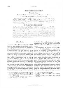
The simulations performed at very small concentrations verified the Fick law with arbitrary small deviations if the space-tine scale is large enough [Vamo¸s et al., 1997b]. Also, using a variable step grid, so that diffusion coefficients where D({k < 0}) = 0.05 and D({k > 0}) = 5.0, one obtains good numerical estimates for the diffusion coefficient (4.12) [Vamo¸s et al. 1998a,b]. Diffusion in random field. The model of Matheron and de Marsily. Similarly with the 1-dimensional case, a random walkers cellular automaton was considered in 2-dimensional grid {xk = kδx, yl = lδy ; −m ≤ k, l ≤ m} [Vamo¸s et al. 2000]. A horizontal random advection, constant in each layer, and Gaussian correlated on the transverse direc2 tion, RE ∼ e−(lδy) , was superposed over the unbiased random walk. Numerical computation reveals a good agreement with the 3/2 law of Matheron and de Marsily [1980]: σx2 (t) = 0.30 t1.53 . Effective diffusion coefficients were estimated through Dx = σx2 (t)/2t and Dy = σy2 (t)/2t. The curves presented in the picture below also agree with the model: Dy const. and 1 Dx const. · t 2 .

15

Dy

Dx

Dx/sqrt(t)

8.0 7.0 6.0 5.0 4.0 3.0 2.0 1.0 0.0 0

20

40

60

80

100

TIME

This is a validity test for the algorithm. If the values of the advection velocities and diffusion coefficients are associated with an advection-diffusion equation, i.e. the advection velocity equals the drift coefficient from the Fokker-Planck equation (3.1) and the local time derivatives of σx2 and σy2 give finite diffusion coefficients (3.4), then the coarse-grained averaged concentration, defined by (4.1) as c 1, gives the numerical solution of the partial derivatives equation. Such models can be further used to study more complex cases of diffusion in random environment, where no analogies between a Langevin (3.3) and FokkerPlanck (3.1) equations are possible. In these cases, the mathematical model for diffusion process is no longer a differential equation, for which one looks for numerical solutions, but it is just the random walkers numerical model, as a computer code.

16

REFERENCES Antoniou, I. and K. E. Gustafson, From Probabilistic Description to Deterministic Dynamics, Physica A 179, 153-166,1993. Antoniou, I. and K. E. Gustafson, From Irreversible Markov Semigroups to Chaotic Dynamics, Physica A 236, 296-308, 1997. Antoniou, I., K. E. Gustafson and Z. Suchanecki, On the Inverse Problem of Statistical Physics: From Irreversible Semigroups to Chaotic Dynamics, Physica A 256, 345-361, 1998. Avellaneda, M., and A. J. Majda, An Integral Representation and Bounds on the Effective Diffusivity in Passive Advection by Laminar and Turbulent Flows, Commun. Math. Phys., 138, 339-391, 1991. B˘alescu, R., Equilibrium and Nonequilibrium Statistical Mechanics, Wiley, New York, 1975. Bianucci, M. R., Mannella, B. J. West and P. Grigolini, From Dynamics to Thermodynamics: Linear response and Statistical Mechanics, Phys. Rev. E 51, 3002, 1995. Boltzmann, L., Scrieri, Ed. S¸tiint¸ific˘a and Enciclopedic˘a, Bucure¸sti, 1981. Bowen, R. M., Porous Media Model Formulation by the Theory of Mixtures, in Fundamentals of Transport Phenomena in Porous Media, J. Bear and M. Y. Corapcioglu (editors), NATO ASI Series E: Applied Sciences, No. 82, Martinus Nijhof Publ., Dordrecht, 1984. Cornfeld, I., S. Fomin and Ya. G. Sinai, Ergodic Theory, Springer, 1982. Crank, J., The Mathematics of Diffusion, Oxford Univ. Press, 1975. Doob, J. L., Stochastic Processes, John Wiley & Sons, London, 1953. Evans, D. J., and G. P. Morriss, Statistical Mechanics of Nonequilibrium Liquids, Academic Press, London, 1990. Fried, J. J., Groundwater Pollution, Elsevier, New York, 1975. Gardiner, C. W., Handbook of Stochastic Methods (for Physics, Chemistry and Natural Science), Springer, New York, 1983. Gaylord, R., and K. Nishidate, Modeling Nature: Cellular Automata and Computer Simulations with Mathematica, Springer, New York, 1996. Hilfer, R., Geometric and Dielectric Characterization of Porous Media, Phys. Rev. B 44, 1, 60-75, 1991. Iosifescu, M. and P. T˘autu, Stochastic Processes and Applications in Biology and Medicine, I Theory, Editura Academiei Bucure¸sti and Springer, Bucure¸sti, 1973. Kirkwood, J. G., Selected Topics in Statistical Mechanics, Gordon and Breach, New York, 1967. 17

Koplik, J. and J. R. Banavar, Continuum Deductions from Molecular Hydrodynamics, Annu. Rev. Fluid Mech., 27, 257-292, 1995. Lasota, A., and M. C. Mackey, Probabilistic Properties of Deterministic Systems, Springer, New York, 1985; second edition: Lasota, A., and M. C. Mackey, Chaos, Fractals, and Noise, Stochastic Aspects of Dynamics, Springer, New York, 1994. Lebowitz, J., Microscopic Origins of the Irreversible Behavior, Physica A 263, 516-527, 1999. Mackey, M. C., The Dynamic Origin of Increasing Entropy, Rev. of. Modern Phys., 61, 4, 981-1016,1989. Matheron,G., and G. de Marsily, Is Transport in Porous Media Always Diffusive?, Water Resour. Res., 16, 901-917,1980. Misra, B., I. Prigogine and M. Courbage, From Deterministic Dynamics to Probabilistic Description, Physica A 98, 1-26, 1979. Monin, A. S., and A. M. Yaglom, Statistical Hydrodynamics I (in Russian) Mir, Moscow, 1965 (translated in English, Statistical Fluid mechanics: Mechanics of Turbulence, MIT Press, Cambridge, M A, 1971). M¨ uller, J., Thermodynamics, Pitman, Boston, 1985. Nishidate, K., M. Baba and R. J. Gaylord, Cellular Automaton Model for Random Walkers, Phys. Rev. Lett., 77 (9), 1675-78, 1996. Onicescu, O., Probabilit˘a¸ti and procese aleatoare, Ed. S¸tiint¸ific˘a and Enciclopedic˘a, Bucure¸sti, 1977. Parisi, G., Systèmes complexes: le point de vue d’un physicien, Physica A 263, 557-564, 1999. Prigogine, I., From Beeing to Becaming, Freeman, San Francisco, 1980. Prigogine, I., Laws of Nature, Probability and Time Symetry Breaking, Physica A 263, 528-539, 1999. Ruelle, D., Gaps and New Ideas in Our Understanding of Nonequilibrium, Physica A 263, 540-544, 1999. Saffman, P. G., Application of the Wiener-Hermite Expansion to the Diffusion of a Passive Scalar in a Homogeneous Turbulent flow, Phys. Fluids 12, 9, 1786-1798, 1969. Sposito, G., The Physics of Soil Water Physics, Water Resour. Res., 22, 9, 83S-88S, 1986. Suciu, N., H. Vereecken, C. Vamo¸s, A. Georgescu, U. Jaekel and O. Neuendorf, On Lagrangian Passive Transport in Porous Media, KFA/ICG-4 Internal report No. 501196, 1996.

18

Suciu, N., C. Vamo¸s, A. Georgescu, U. Jaekel and H. Vereecken, Coarse Grained and Stochastic Averages. Applications to Transport Processes in Porous Media, Forschungszentrum J¨ ulich, ICG-4, Internal Report No. 500198, 1998a. Suciu, N, C. Vamo¸s, A. Georgescu, U. Jaeckel, H. Vereecken, Transport processes in porous media. 1. Continuous modeling, Rom J. of Hydr. & Water Resour. 5, No. 1-2, 39-56, 1998b. Sz-Nagy, B and C. Foia¸s, Harmonic Analysis of Operators in Hilbert Spaces, North-Holland, Amsterdam, 1970. Taylor, G. I., Diffusion by Continuous Movements, Proc. London Math. Soc., 2, 20, 196-212, 1921. Vamo¸s, C., A. Georgescu, N. Suciu and I. Turcu, Balance Equations for Physical Systems with Corpuscular Structure, Physica A 227, 81-92, 1996a. Vamo¸s, C., A. Georgescu and N. Suciu, Balance Equations for a Finite Number of Particles, Stud. Cerc. Mat. 48, 1-2, 115-127, 1996b. Vamo¸s, C. and N. Suciu, Simularea numeric˘a a difuziei la concentrat¸ii mici, Contract Nr. 7006/1996, GAR-31/1996. Vamo¸s, C., N. Suciu and A. Georgescu, Hydrodynamic Equations for One-Dimensional Systems of Inelastic Particles, Phys. Rev. E 55, 5, 6277-6280, 1997a. Vamo¸s, C., N. Suciu and M. Peculea, Numerical Modelling of the Pne-Dimensional Diffusion by Random Walkers, Rev. Anal. Numér. Thèorie Approximation, 26, 1-2, 237-247, 1997b. Vamo¸s, C., N. Suciu, U. Jaekel and H. Vereecken, Numerical Modelling of Diffusion Processes by Cellular Automata, Forschungszentrum J¨ ulich, ICG-4, Internal Report No. 501198, 1998a. Vamo¸s,C., N. Suciu, U. Jaeckel, H. Vereecken, Transport processes in porous media. 2. Numerical modeling, Rom J. of Hydr. & Water Resour. 5, No. 1-2, 85-98, 1998b. Vamo¸s, C., N. Suciu, H. Vereecken, U. Jaekel and H. Schwarze, Random Walkers Cellular Automata for Diffusion Processes, Z. Angew. Math. Mech. 80, S2, S367-68, 2000.

19