during a time interval ." "Survey region (set of places) during the interval of time ." "Signal the detection of event within a region during the interval ." Before execution, each task is decomposed into a sequence of subgoals which comprise a plan. Advance planning permits the system to estimate the resources required for the mission. Because the environment is not perfectly known in advance, the decomposition of the task is not sure to succeed. To successfully execute a mission, the supervisor must monitor the execution of each task and dynamically generate the actions required to accomplish its goals. Both planning and plan execution are knowledge intensive processes which are adapted to a forward chaining production system. The supervisor on our surveillance robot has been implemented using a rule based language (CLIPS 6.0) to which we have added an asynchronous message passing facility [Crowley 87]. The supervisor plans navigation actions using a network of named places connected by named routes. Each place contains its location in an local reference frame, as well as a list of places which are directly accessible by a straight line routes. Each route is described by a data structure which contains information about appropriate navigation procedures, speeds, path length, and surveillance behaviours which are appropriate for the route. The supervisor commands navigation "actions" in order to accomplish the tasks in its mission. The 4
set of navigation actions are based on the use of a vehicle level controller which independently servos translation and rotation.
2.3 Control of Translation and Rotation: The Standard Vehicle Controller Robot arms require an "arm controller" to command joint motors to achieve a coordinated motion in an external Cartesian coordinate space. In the same sense, robot vehicles require a "vehicle controller" to command the motors to achieve a coordinated motion specified in terms of an external Cartesian coordinate space. The locomotion procedures describes below are based on the LIFIA "standard vehicle controller" which provides asynchronous independent control of forward displacement and orientation [Crowley 89b]. A production version of this controller is in everyday use in our laboratory. This controller is the subject of section 3 below. Position estimation includes a model of the errors of the position estimation process. Thus the estimated position is accompanied by an estimate of the uncertainty, in the form of a covariance matrix. This covariance matrix makes it possible to correct the estimated position using a Kalman Filter. This correction is provided as a side effect in the process of dynamic modeling of the local environment.
2.4 Dynamic Modeling with Ultrasonic Range Sensors Perception serves two fundamentally important roles for navigation: 1) Detection of the limits to free space, and 2) Position estimation. Free space determines the set of positions and orientations that the robot may assume without "colliding" with other objects. Position estimation permits the robot to locate itself with respect to goals and knowledge about the environment. Our navigation system employs a dynamically maintained model of the environment of the robot using ultrasonic sensors and a pre-stored world model [Crowley 89a]. We call such a model a "composite local model". Such a model is "composite" because it is composed of several points of view and (potentially) several sources. The model is local, because it contains only information from the immediate environment. The modeling process is illustrated in figure 2.2. Raw sensor data is processed to produce an immediately perceived description of the environment in terms of a set of geometric primitives expressed in a common external coordinate system. Data are currently provided from the ultrasonic range sensors. We have also developed a real time stereo system [Crowley 91]. Sonar interpretation uses coherence in the data to determine a subset of the measurements which are reliable.
5
The composite model describes the limits to free space which are currently visible to the robot. The contents of the composite model are never directly available to the other parts of the system. Instead the contents are accessible through a set of interface procedures which interrogate the composite model and return both symbolic information and geometric parameters. Ultrasound Sensor Data Pre-learned World Model ∆P, Kp
°°°
Stereo Sensor Data
Match Position Correction
Predict
Update Composite Local Model Figure 2.2 An abstraction description of sensor data is used to dynamically update a composite model of the limits to free space. The problem of combining observations into a coherent description of the world is basic to perception. In this paper, we present a framework for vehicle control, position estimation, and perception which is based on maintaining an explicit model of the precision (or uncertainty) of all parameters. We argue that for numerical data, techniques from estimation theory may be directly adapted to the problem. For symbolic data, these principles suggest an adaptation of certain existing techniques for the problem of perceptual fusion. The following section reviews the mathematical foundations from estimation on which this framework is based.
6
3 Mathematical Foundations from Estimation Theory In order to plan and execute actions in a reliable manner, an autonomous robot must reason about its environment. For this, the robot must have a description of the environment. This description is provided by fusing "perceptions" from different sensing organs (or different interpretation procedures) obtained at different times. We define perception as: The process of maintaining of an internal description of the external environment. The external environment is that part of the universe which is accessible to the sensors of an agent at an instant in time. In theory, it would seem possible to use the environment itself as the internal model. In practice, this requires an extremely complete and rapid sensing ability. It is far easier to build up a local description from a set of partial sources of information and to exploit the relative continuity of the universe with time in order to combine individual observations. We refer to the problem of maintaining an internal description of the environment as a that of "Dynamic World Modeling". By dynamic we mean that the description evolves over time based on information from perception. This description is a model, because it permits the agent to "simulate" the external environment. This use of model conflicts with "models" which a systems designer might use in building a system. This unhappy confusion is difficult to avoid given that the two uses of "model" are thoroughly embedded in the vocabulary of the scientific community. This confusion is particularly troublesome in the area of perceptual fusion, where a sensor "model" is necessary for the proper design of the system, and the result of the system is to maintain a world "model". Having signaled this possible confusion, we will continue with the terminology which is common in the vision and robotics communities: the use of “model” for an internal description used by a system to reason about the external environment.
3.1 Background Recent advances in sensor fusion for mobile robotics have largely entailed the rediscovery and adaptation of techniques from estimation theory. These techniques have made their way to vision via the robotics community, with some push from military applications. For instance, in the early 1980's, Herman and Kanade [Herman-Kanade 86] combined passive stereo imagery from an aerial sensor. This early work characterized the problem as one of incremental combination of geometric information. A similar approach was employed by the author for incremental construction of world model of a mobile robot using a rotating ultrasonic sensor 7
[Crowley 85]. That work was generalized [Crowley 92] to present fusion as a cyclic process of combining information from logical sensors. The importance of an explicit model of uncertainty was recognized, but the techniques were for the most part "ad-hoc". Driven by the needs of perception for mobile robotics, Brooks [Brooks 85] and Chatila [Chatila-Laumand 85] also published ad-hoc techniques for manipulation of uncertainty. In 1985, a pre-publication of a paper by Smith and Cheeseman was very widely circulated [SmithCheeseman 87]. In this paper, the authors argue for the use of Bayesian estimation theory in vision and robotics. An optimal combination function was derived and shown to be equivalent to a simple form of Kalman filter. At the same period, Durrant-Whyte completed a thesis [Durrant-Whyte 87] on the manipulation of uncertainty in robotics and perception. This thesis presents derivations of techniques for manipulating and integrating sensor information which are extensions of technique from estimation theory. Well versed in estimation theory, Faugeras and Ayache [Faugeras et al 86], [Ayache-Faugeras 87] contributed an adaptation of this theory to stereo and calibration. Dickmanns demonstrated the use of a Kalman Filter for perception and control in automatic driving [Dickmanns 88]. From 1987, a rapid paradigm shift occurred in the vision community, with techniques from estimation theory being aggressively adapted. While most researchers applying estimation theory to perception can cite one of the references [SmithCheeseman 87], [Durrant-Whyte 87] or [Faugeras et al 86] for their inspiration, the actual techniques were well known to some other scientific communities, in particular the community of control theory. The starting point for estimation theory is commonly thought to be the independent developments of Kolmogorov [Kolmogorov 41] and Weiner [Weiner 49]. Bucy [Bucy 59] showed that the method of calculating the optimal filter parameters by differential equation could also be applied to non-stationary processes. Kalman [Kalman 60] published a recursive algorithm in the form of difference equations for recursive optimal estimation of linear systems. With time, it has been shown that these optimal estimation methods are closely related to Bayesian estimation, maximum likelihood methods, and least squares methods. These relationships are developed in textbooks by Bucy and Joseph [BucyJoseph 68], Jazwinski [Jazwinski 70], and in particular by Melsa and Sage [Melsa-Sage 71]. These relations are reviewed in a recent paper by Brown et. al. [Brown et al 89], as well as in a book by Brammer and Siffling [Brammer-Siffling 89]. These techniques from estimation theory provide a theoretical foundation for the processes which compose the proposed computational framework for fusion in the case of numerical data. An alternative approach for such a foundation is the use of minimum energy or minimum entropy criteria. An example of such a computation is provided by a Hopfield net [Hopfield 82]. The idea is to minimize some sort of energy function that expresses quantitatively by how much each available measurement and each imposed constraint are violated [Li 89]. This idea is related to regularization techniques for surface reconstruction employed by Terzopoulos [Terzopoulos 86]. The implementation of regularization algorithms using massively parallel neural nets has been discussed 8
by Marroquin, Koch et. al. [Koch et al 85], Poggio and Koch [Koch-Poggio 85] and Blake and Zisserman [Blake-Zisserman 87]. Estimation theory techniques may be applied to combining numerical parameters. In this paper, we propose a computational framework which may be applied to numeric or symbolic information. In the case of symbolic information, the relevant computational mechanisms are inference techniques from artificial intelligence. In particular, fusion of symbolic information will require reasoning and inference in the presence of uncertainty using constraints. The Artificial Intelligence community has developed a set of techniques for symbolic reasoning. In addition to brute force coding of inference procedures, rule based "inference engines" are widely used. Such inference may be backward chaining for diagnostic problems, consultation, or data base access as in the case of MYCIN [Buchanan-Shortliffe 84]. Rule based inference may also be forward chaining for planning or process supervision, as is the case in OPS5 [Brownston et al 85]. Forward and backward chaining can be combined with object-oriented "inheritance" scheme as is the case in KEE and in SRL. Groups of "experts" using these techniques can be made to communicate using black-board systems, such as BB1 [Hayes-Roth 85]. For perception, any of these inference techniques must be used in conjunction with techniques for applying constraint based reasoning to uncertain information. Several competing families of techniques exist within the AI community for reasoning under uncertainty. Automated Truth Maintenance Systems [Doyle 79] maintain chains of logical dependencies, when shifting between competing hypotheses. The MYCIN system [BuchananShortliffe 84] has made popular a set of ad-hoc formulae for maintaining the confidence factors of uncertain facts and inferences. Duda, Hart and Nilsson [Duda et al 76] have attempted to place such reasoning on a formal basis by providing techniques for symbolic uncertainty management based on Bayesian theory. Shafer has also attempted to provide a formal basis for inference under uncertainty by providing techniques for combining evidence [Shafer 84]. A large school of techniques known as "Fuzzy Logic" [Zadeh 79] exist for combining imprecise assertions and inferences.
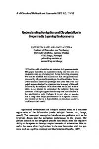
3.2 A General Framework for Dynamic World Modeling A general framework for dynamic world modeling is illustrated in figure 3.1. In this framework, independent observations are "transformed" into a common coordinate space and vocabulary. These observations are then integrated (fused) into a model (or internal description) by a cyclic process composed of three phases: Predict, Match and Update.
9
Observation
Transformation
Common Vocabulary Match Update Predict
Model
Figure 3.1. A Framework for Dynamic World Modeling. Predict: In the prediction phase, the current state of the model is used to predict the state of the external world at the time that the next observation is taken. Match: In the match phase, the transformed observation in brought into correspondence with the predictions. Such matching requires that the observation and the prediction express information which is qualitatively similar. Matching requires that the predictions and observations be transformed to the same coordinate space and to a common vocabulary. Update: The update phase integrates the observed information with the predicted state of the model to create an updated description of the environment composed of hypotheses. The update phase serves both to add new information to the model as well as to remove "old" information. During the update phase, information which is no longer within the "focus of attention" of the system, as well as information which has been found transient or erroneous, is removed from the model. This process of "intelligent forgetting" is necessary to prevent the internal model from growing without limits. We have demonstrated systems in which this framework is applied to maintain separate models of the environment with different update rates and information at different levels of abstraction. For example, in the SAVA Active Vision System [Crowley 91], dynamic models are maintained for edge segments in image coordinates, for 3D edges in scene coordinates and of symbolic labels of recognized objects. In the MITHRA surveillance robot system [Crowley 87], a geometric model of the environment is maintained in world coordinates, and a separate symbolic model is maintained based on searching the geometric model to detected expected objects. 10
From building systems using this framework, we have identified a set of principles for integrating perceptual information. These principles follow directly from the nature of the cyclic process for dynamic world modeling.
3.3 Principles for Integrating Perceptual Information Experience from building systems for dynamic world modeling have led us to identify a set of principles for integrating perceptual information. These principles follow directly from the nature of the "predict-match-update" cycle presented in figure 3.2. Principle 1) Primitives in the world model should be expressed as a set of properties. A model primitive expresses an association of properties which describe the state of some part of the world. This association is typically based on spatial position. For example the co-occurrence of a surface with a certain normal vector, a yellow colour, and a certain temperature. For numerical quantities, each property can be listed as an estimate accompanied by a precision. For symbolic entities, the property slot can be filled with a list of possible values, from a finite vocabulary. This association of properties is known as the "state vector" in estimation theory. Principle 2) Observation and Model should be expressed in a common coordinate system. In order to match an observation to a model, the observation must be "registered" with the model. This typically involves transforming the observation by the "inverse" of the sensing process, and thus implies a reliable model of the sensor geometry and function. When no prior transformation exists, it is sometimes possible to infer the transformation by matching the structure of an observation to the internal description. In the absence of a priori information, such a matching process can become very computationally expensive. Fortunately, in many cases an approximate registration can be provided by knowledge that the environment can change little between observations. The common coordinate system may be scene based or observer based. The choice of reference frame should be determined by considering the total cost of the transformations involved in each predictmatch-update cycle. For example, in the case of a single stationary observer, a sensor based coordinate system may minimize the transformation cost. For a moving observer with a model which is small relative to the size of the observations, it may be cheaper to transform the model to the current sensor coordinates during each cycle of modeling. On the other hand, when the model is large compared to the number of observations, using an external scene based system may yield fewer computations. 11
Transformations between coordinate frames generally require a precise model of the entire sensing process. This description, often called a “sensor model”, is essential to transform a prediction into the observation coordinates, or to transform an observation into a model based coordinate system. Determining and maintaining the parameters for such a “sensor model” is an important problem which is not addressed in this paper. Principle 3) Observation and model should be expressed in a common vocabulary. A perceptual model may be thought of as a data base. Each element of the data base is a collection of associated properties. In order to match or to add information to a model, an observation needs some be transformed to the terms of the data base in order to serve as a key. It is possible to calculate such information as needed. However since the information is used both in matching and in updating, it makes more sense to save it between phases. Thus we propose expressing the observation in a subset of the properties used in the model. An efficient way to integrate information from different sensors is to define a standard "primitive" element which is composed of the different properties which may be observed or inferred from different sensors. Any one sensor might supply observations for only a subset of these properties. Transforming the observation into the common vocabulary allows the fusion process to proceed independent of the source of observations. Principle 4) Properties should include an explicit representation of uncertainty. Dynamic world modeling involves two kinds of uncertainty: precision and confidence. Precision can be thought of as a form of spatial uncertainty. By explicitly listing the precision of an observed property, the system can determine the extent to which an observation is providing new information to a model. Unobserved properties can be treated as observations which are very imprecise. Having a model of the sensing process permits an estimate of the uncertainties to be calculated directly from the geometric situation. Principle 5) Primitives should be accompanied by a confidence factor. Model primitives are never certain; they should be considered as hypotheses. In order to best manage these hypotheses, each primitive should include an estimate of the likelihood of its existence. This can have the form of a confidence factor between -1 and 1 (such as in MYCIN [Buchanan-Shortliffe 84]), a probability, or even a symbolic state from a finite set of confidence state. A confidence factor provides the world modeling system with a simple mechanism for non-monotonic reasoning. Observations which do not correspond to expectations may be initially considered as 12
uncertain. If confirmation is received from further observation, their confidence is increased. If no further confirmation is received, they can be eliminated from the model. The application of these principles leads to a set of techniques for the processes of dynamic world modeling. In the next section we discuss the techniques for the case of numerical properties, and provide examples from systems in our laboratory.
3.4 Techniques for Fusion of Numerical Properties In the case of numerical properties, represented by a primitive composed of a vector of property estimates and their precisions, a well defined set of techniques exists for each of the phases of the modeling process. In this section we show that the Kalman filter prediction equations provides the means for predicting the state of the model, the Mahalanobis Distance provides a simple measure for matching, and the Kalman filter update equations provide the mechanism to update the property estimates in the model. We also discuss the problem of maintaining the confidence factor of the property vectors which make up the model. A dynamic world model, M(t), is a list of primitives which describe the "state" of a part of the world at an instant in time t. Model:
M(t) ≡ { P 1(t), P 2(t),... , P m(t)}
A model may also include "grouping" primitives which assert relations between lower level primitives. Examples of such groupings include connectivity, co-parallelism, junctions and symmetry. Such groupings constitute abstractions which are represented as symbolic properties. Each primitive, Pi(t), in the world model, describes a local part of the world as a conjunction of ^ estimated properties, X (t), plus a unique ID and a confidence factor, CF(t). Primitive :
P(t) ≡ {ID, X^ (t), CF(t)}
The ID of a primitive acts as a label by which the primitive may be identified and recalled. The confidence factor, CF(t), permits the system to control the contents of the model. Newly observed segments enter the model with a low confidence. Successive observations permit the confidence to increase, where as if the segment is not observed in the succeeding cycles, it is considered as noise and removed from the model. Once the system has become confident in a segment, the confidence factor permits a segment to remain in existence for several cycles, even if it is obscured from observations. Experiments with have lead us to use a simple set of confidence "states" represented by integers. The number of confidence states depends on the application of the system.
13
A primitive represents an estimate of the local state of a part of the world as an association of a set of ^ N properties, represented by a vector , X (t). X^ (t) ≡ { x^ 1(t), x^2(t),... x^n(t)}. The actual state of the external world, X(t), is estimated by an observation process YH X which projects the world onto a observation vector Y(t). The observation process is generally corrupted by random noise, N(t). Y(t) =
Y XH
X(t) + N(t).
The world state, X(t), is not directly knowable, and so our estimate is taken to be the expected value ^ X^ (t) built up from observations. At each cycle, the modeling system produces an estimate X (t) by combining a predicted observation, Y*(t), with an actual observation Y(t). The difference between the predicted vector Y*(t) and the observed vector Y(t) provides the basis for updating the estimate X^ (t), as described below. ^ In order for the modeling process to operate, both the primitive, X (t) and the observation, Y(t) must be accompanied by an estimate of their uncertainty. This uncertainty may be seen as an expected ^ deviation between the estimated vector, X (t), and the true vector, X(t). Such an expected deviation is ^ approximated as a covariance matrix C (t) which represents the square of the expected difference between the estimate and the actual world state.
C^ (t) ≡ E{[X(t) – X^ (t)] [X(t) – X^ (t)}] T} Modeling this precision as a covariance makes available a number of mathematical tools for matching and integrating observations. The uncertainty estimate is based on a model of the errors which corrupt the prediction and observation processes. Estimating these errors is both difficult and essential to the function of such a system. The uncertainty estimate provides two crucial roles: 1) It provides the tolerance bounds for matching observations to predictions, and 2) It provides the relative strength of prediction and observation when calculating a new estimate. Because C^ (t) determines the tolerance for matching, system performance will degrade rapidly if we under-estimate C^ (t). On the other hand, overestimating C^ (t) may increase the computing time for finding a match.
3.5 Prediction: Discrete State Transition Equations 14
The prediction phase of the modeling process projects the estimated vector X^ (t) forward in time to a predicted value, X*(t+∆T). This phase also projects the estimated uncertainty C^ (t) forward to a predicted uncertainty C*(t+∆T). Such projection requires estimates of the temporal derivatives for the ^ properties in X (t), as well as estimates of the covariances between the properties and their derivatives. ^ These estimated derivatives can be included as properties in the vector X (t). In the following, we will describe the case of a first order prediction; that is, only the first temporal derivative is estimated. Higher order predictions follow directly by estimating additional derivatives. We will illustrate the techniques for a primitive composed of two properties, x1(t) and x2(t). We employ a continuous time variable t to mark the fact that the prediction and estimation may be computed for a time interval, ∆T, which is not necessarily constant. Temporal derivatives of a property are represented as additional components of the vector X(t). Thus, if a system estimates N properties, the vector X(t) is composed of 2N components: the N properties and N first temporal derivatives. It is not necessary that the observation vector, Y(t), contain the derivatives of the properties to be estimated. The Kalman filter permits us to iteratively estimate the derivatives of a property using only observations of its value. Furthermore, because these estimates are developed by integration, they are more immune to noise than instantaneous derivatives calculated by a simple difference. ^ Consider a property, x^ (t), of the vector X (t), having variance σ^ 2x. A first order prediction of the value
x*(t+∆T) requires an estimate of the first temporal derivative, ^x'(t). ∂x^ (t) x^ ' (t) ≡ ∂t The evolution of X(t) can be predicted by a Taylor series expansion. To apply a first order prediction, all of the higher order terms are grouped into an unknown random vector V(t), ^ ^ approximated by an estimate, V (t). The term V (t) models the effects of both higher order derivatives and other unpredicted phenomena. V(t) is defined to have a variance (or energy) of Q(t). Q(t) = E{V(t) V(t)T} When V(t) is unknown, it is assumed to have zero mean, and thus is estimated to be zero. However, in some situation it is possible to estimate the perturbation from knowledge of commands by an ^ associated control system. In this case, an estimated perturbation vector V (t) and its uncertainty, Q^(t) may be included in the prediction equations. Thus each term is predicted by:
15
x*(t+∆T) = x^ (t) +
∂x^ (t) ^ ∂t ∆T + v(t)
^ Let us consider a vector, X (t), composed of the properties x^ 1(t) and x^ 2(t) and their derivatives.
X^ (t) ≡
x^1(t) ^ xx^12'(t) (t) x^ '(t) 2
In matrix form, the prediction can be written as: X*(t+∆T) :=
ϕ X^ (t) + V^ (t)
The time increment ∆T is included in the transition matrix, ϕ.
ϕ
≡
1 ∆T 0 1 0 0 0 0
0 0 1 0
0 0 ∆T 1
This gives the prediction equation in matrix form: X*(t+∆T) :=
ϕ X^ (t) + V^ (t)
(1)
Predicting the uncertainty of X*(t+∆T) requires an estimate of the covariance between each property, x^ (t) and its derivative. ^ An estimate of this uncertainty, Q x(t), permits us to account for the effects of unmodeled derivatives when determining matching tolerances. This gives the second prediction equation: ^ Cx* (t+∆T) := ϕT C^ x(t) ϕ + Q x(t)
(2)
3.6 Matching Observation to Prediction: The Mahalanobis Distance The predict-match-update cycle presented in this paper simplifies the matching problem by applying the constraint of temporal continuity. That is, it is assumed that during the period ∆T between observations, the deviation between the predicted values and the observed values of the estimated primitives is small enough to permit a trivial "nearest neighbour" matching. Let us define a matrix YX H which transforms the coordinate space of the estimated state, X(t), to the coordinate space of the observation. 16
Y(t) =
Y XH
X(t) + W(t)
The matrix YX H constitutes a "model" of the sensing process which predicts an observation, Y(t) given knowledge of the properties X(t). Estimating YX H is a crucial aspect of designing a world modeling system. The model of the observation process, YX H, can not be assumed to be perfect. In machine vision, the observation process is typically perturbed by photo-optical, optical and electronic effects. Let us define this perturbation as W(t). In most cases, W(t) is unknown, leading us to estimate: ^ W (t) ≡ E{W(t)} = 0
and: C^ y(t) ≡ E{ W(t) W(t) T} To illustrate this process, suppose that we can observe the current value of two properties but not their derivatives. In this case YX H, can be used to yield a vector removing the derivatives from the predicted properties. The two-property, first order vector used in the example from the previous section would give a prediction YX H of:
y1*(t) = y2*(t)
[ 01
0 0
0 1
0 0
]
x1*(t) * xx12*'(t) (t) x *'(t) 2
Of course YX H may represent any linear transformation. In the case where the estimated state and the observation are related by a transformation, F(X), which is not linear, YX H is approximated by the first derivative, or Jacobian, of the transformation, YX J . Y XJ
=
∂F(X) ∂X
Let us assume a predicted model M*(t) composed of a list of primitives, P*n(t), each containing a parameter vector, X*(t), and an observed model O(t) composed of a list of observed primitives, Pm(t), each containing the parameters Y(t). The match phase determines the most likely association of observed and predicted primitives based on the similarity between the predicted and observed properties. The mathematical measure for such similarity is to determine the difference of the properties, normalized by their covariance. This distance, normalized by covariance, is a quadratic form known as the squared Mahalanobis distance. The predicted parameter vector is given by: 17
Yn* :=
Y XH
Xn*
(3)
with covariance * := Y * Cyn X H C xn
Y T XH
(4)
The observed properties are Ym with covariance Cym. The squared Mahalanobis distance between the predicted and observed properties is given by: 2 Dnm =
1 T * -1 * * 2 { (Yn – Ym) (Cyn + Cym) (Yn – Ym)}
For the case where a single scalar property is compared, this quadratic form simplifies to:
1 (yn* – y m)2 2 Dnm = 2 (σy*2n +σy2m ) In the predict-match-update cycles described below, matching involves minimizing the normalized distance between predicted and observed properties or verifying that the distance falls within a certain number of standard deviations. The rejection threshold for matching depends on the trade-off between the risk of rejecting a valid primitive, as defined by the Χ2 square distribution and the desire to eliminate false matches. For example, for a single 1-D variable, to be sure to not reject 90% of true matches, the normalized distance should be smaller than 2.71. For 95% confidence, the value is 3.84. As the probability of not rejecting a good match goes up, so does the probability of false alarms.
3.7 Updating: The Kalman Filter Update Equations Having determined that an observation corresponds to a prediction, the properties of the model can be updated. The extended Kalman filter permits us to estimate a set of properties and their derivatives, X^n(t), from the association of a predicted set of properties, Yn*(t), with an observed set of properties, Ym(t). It equally provides an estimate for the precision of the properties and their derivatives. This estimate is equivalent to a recursive least squares estimate for Xn(t). The estimate and its precision will converge to a false value if the observation and the estimate are not independent. The crucial element of the Kalman filter is a weighting matrix known as the Kalman Gain, K(t). The Kalman Gain may be defined using the prediction uncertainty C*y(t). 18
K(t) := C*x(t)
Y T XH
[ C*y(t) + Cy(t)] -1
(5)
The Kalman gain provides a relative waiting between the prediction and observation, based on their relative uncertainties. The Kalman gain permits us to update the estimated set of properties and their derivatives from the difference between the predicted and observed properties: X^(t) := X*(t) + K(t) [Y(t) – Y*(t)]
(6)
The precision of the estimate is determined by: C^ (t) := C*(t) – K(t) YX H C*(t)
(7)
Equations (1) through (7) constitute the 7 equations of the Kalman Filter. For primitives composed of numerical properties, the Kalman filter equations provide the tools for our framework.
3.8 Eliminating Uncertain Primitives and Adding New Primitives to the Model Each primitive in the world model should contain a confidence factor. In most of our systems we represent confidence by a discrete set of five states labelled as integers. This allows us to emulate a temporal decay mechanism, and to use arbitrary rules for transitions in confidence. During the update phase, the confidence of all model primitives is reduced by 1. Then, during each cycle, if one or more observed token is found to match a model token, the confidence of the model token is incremented by 2, to the maximum confidence state. After all of the model primitives have been updated, and the model primitives with CF = 0 removed from the model, new model primitives are created for each unmatched observed primitives. When no model primitive is found for an observed primitive, the observed primitive is added to the model with the observed property estimates and a temporal derivative of zero. The covariances are set to large default values and the confidence factor is set to 1. In the next cycle, a new primitive has a significant possibility of finding a false match. False matches are rapidly eliminated, however, as they lead to incorrect predictions for subsequent cycles and a subsequent lack of matches. Because an observed primitive can be used to update more than one model primitive, such temporary spurious model primitives do not damage the estimates of properties of other primitives in the model.
4 A Kalman Filter Based Vehicle Controller Robot arms require an "arm controller" to command joint motors to achieve a coordinated motion in 19
an external Cartesian coordinate space. In the same sense, robot vehicles require a "vehicle controller" to command the motors to achieve a coordinated motion specified in terms of an external Cartesian coordinate space. In this section we describing a vehicle controller based on a Kalman filter. This vehicle controller provides asynchronous independent control of forward translation and rotation. The controller accepts both velocity and displacement commands, and can support a diverse variety of navigation techniques. In addition, the controller operates in terms of a standardized "virtual vehicle" which may be easily adapted to a large variety of vehicle geometries. All vehicle specific information is contained in the low level interface which translates the virtual vehicle into a specific vehicle geometry. Early versions of this controller have been developed for the CMU Terragator, the Denning DRV-1 and the TRC Labmate. This controller has been in every-day use in our laboratory on a RobotSoft Robuter since 1988. This first section presents an overview of the vehicle controller as a three layer structure. This is followed by descriptions of the command interpreter and the techniques for estimating vehicle position and generating vehicle commands. A description is then given of the translator for a differentially steered vehicle. Versions of this controller have been in everyday use in a vehicle in our laboratory since 1988. The standard vehicle controller is organised in three layers, as illustrated in figure 2.1. The top layer is a set of procedures which interpret command strings in order to set the value of control parameters or return information about the vehicle's position or velocity. Commands are directly translated into calls to a set of interface procedures. These interface procedures provide an alternative command interface for processes running on the same processor. The inner layer is a control loop composed of two parts. One part updates an estimate of the vehicle's pose, covariance, and state vector. The second part compares the observed displacement to the control parameters and generates new orders for the motors of a "virtual vehicle". Because, the vehicle controller operates in terms of a standardized "virtual vehicle" and thus may be easily adapted to a large variety of vehicle geometries.
4.1 A Kalman Filter model for odometric position estimation The vehicle controller estimates and commands a state vector composed of the incremental translation and rotation (S, α) and their derivatives.
U =
S'S α α' 20
The controller also maintains estimates of the absolute position and orientation (the pose) and its uncertainty, represented by a covariance. The "pose" of a vehicle is defined as the estimated values for position and orientation: xr X^ ≡ yr θ r The uncertainty in pose is represented by a covariance matrix:
^
CX ≡
σx2 σyx σθx σxy σy2 σθy σxθ σyθ σθ2
The bottom layer, called the translator, provides a virtual vehicle interface for a particular vehicle geometry. This layer is composed of two parts. One part reads the values of the motor encoders and translates the incremental change into a change in position and orientation of the vehicle. The second part receives orders for changes in the velocity of orientation and position of the vehicle, and translates these into velocity commands for the motors. Protocol Interpretation Commanded State
1
Estimated State
State Parameters
3 Command Generation
2 State Estimation
4
Virtual Vehciel
Translation (Virtual Vehicle to Real Vehicle) Figure 4.1 Organisation of the Standard Vehicle Controller. The bottom layer is a translator which converts a specific vehicle geometry into a "virtual vehicle". The middle layer is a control loop which estimates and commands the vehicle's translation and orientation. The top layer is a command interpreter .
4.2 External Interface Protocol The vehicle controller responds to six commands. Three of these commands refer to movement of the vehicle. 21
m[ove] [d[, v[, a]]]
"Move" with speed v meters/sec, for a maximum distance of d meters, and an acceleration of a meters/sec2.
t[urn] [d[, v[, a]]]
Turn with a angular speed of v degrees/sec, for a maximum rotation of d degrees, and an angular acceleration of a degrees/sec2.
Stop
Stop all motion and hold the current position and orientation.
Brackets "[]" indicate optional parameters or letters. A command without parameters will take the last specified value as a default. A command to move or turn replaces the current reference values for the servo and thus takes effect immediately. The vehicle control loop uses twin data structures for translation and rotation. Commands to move, turn or stop set new values for the commanded displacement, speed and acceleration within these structures. The finite state machines for move and for turn are independent, so that commands to one does not interfere with a command to the other. Both commands are cancelled by a command to stop. A command to move or stop will reset the accumulated translation and its derivatives (s, s') to zero, while a command to turn or stop will reset accumulated rotation and its derivative (α, α'). This protocol allows independent locomotion procedures for movement and steering to drive the vehicle. For example, a translation process initializes movement by specifying a move with a speed and maximum distance. Then at regular intervals, the process verifies that no obstacle is present and sends a command "m" without parameters, thereby resetting the accumulated distance. Independently, a steering process periodically measures the error between the desired and actual heading, and issues a turn command with the desired correction angle, and a velocity based on the maximum permissible curvature for the current speed. The "pose" of the vehicle is its position and orientation. Commands which refer to the estimated position and velocity of the vehicle are: GetEstPos
Return the estimated pose, (x, y, θ), and Covariance Cx.
GetEstSpeed
Return the estimated speed of the vehicle vs, v α .
CorrectPos ∆Y, K x
Correct the pose by ∆Y using the Kalman filter gain matrix K x.
ResetPos X, Cx
Set the pose and covariance to the specified values.
22
The commands to "get" the estimated position or velocity returns the current values for position, covariance, or velocity. The command to reset the position and covariance is useful for initialization and for testing the position correction. The command to correct the estimated position applies a Kalman filter to the position using the "innovation" ∆Y. ^ ^ X := X + K ∆Y. ^ ^ C X := CX - K C X
The Kalman Gain matrix is a 3 by 3 matrix which tells how much of the change in each parameter should be taken into account in correcting the other parameters. Experiments in using an extended Kalman filter to estimate position using ultrasonic range sensors is described in [Crowley 89a]. Experiments with the use of vision to measure the angle to a known vertical structure to correct position are described in [Chenavier-Crowley 92]. A review of the use of Kalman filters for world modeling and estimation is given in [Crowley et al 92]. The process for estimating the vehicle's pose and uncertainty from odometry are described below. The use of different sensing modalities to compute the Kalman gain and innovation are described in the next section.
4.3 The Inner Control Loop The inner control loop is composed of two parts: Position estimation and generation of motor commands. The position estimation process maintains an estimate of the vehicle's current position and velocity, as well as their uncertainties. The command process generates velocity commands for forward displacement and orientation for a "virtual vehicle". The inner control loop is actually composed of two independent copies of the same control process: one copy controls forward displacement while the second copy controls orientation. For both forward displacement and orientation displacement, the control loop is organized as a finite state machine with the four states, as illustrated in figure 4.1. These four state are: HOLD: ACCEL: DECCEL: MOVE:
Act so as to maintain the current displacement. Linearly increase the speed to a specified value. Linearly decrease the speed to a specified value. Maintain a specified velocity
In the HOLD state, the process controls the value of a parameter. That is, the control process acts to maintain the accumulated forward displacement or accumulated orientation equal to zero. In states ACCEL, MOVE, and DECCEL the control process servos the first temporal derivative of a parameter.
23
HOLD state is particularly useful for maintaining a desired heading when starting a forward displacement, or for holding a position while turning. For example, accelerating at the beginning of a forward displacement provokes an error in orientation. This error is detected, and corrected by the command process for orientation. The DECCEL state decreases the velocity of the vehicle so that it comes to a halt at the distance or orientation specified in the move or turn command. The movement and orientation control loops require measured values for both instantaneous speed and for accumulated displacement. These are provided by the position estimation process.
speed v + ∆v v
v - ∆v ACCEL
MOVE
DECCEL
HOLD time
Figure 4.2 States of the command process. This process is operates independently for both the forward movement and rotation.
4.4 Estimating Position and Uncertainty. The odometric position estimation process is activated at a regular interval by a real time scheduler. The process requests the translator to provide the change in the translation, ∆S, and rotation, ∆α, since the last call. The process also reads the system real-time clock to determine the change in time, ∆T, since the last call. The accumulated translation and rotation are calculated as: S := S + ∆S α := α + ∆α The derivatives of the translation and rotation are calculated as: ∆S S' := ∆T ∆α α' := ∆T
24
Accelerations are used to estimate the uncertainty in vehicle position and orientation. At each cycle, the position estimation procedure calculates the accelerations in translation and rotation as the difference in the instantaneous velocities. S' t – S ' t-1 ∆T α' t – α' t-1 α'' = ∆T S'' =
In order to update the pose, we assume that the rotational speed of the vehicle is constant within a cycle of the estimation process. Thus the average orientation during a cycle is given by the previous estimate plus half the incremental change. ∆α θ = θ^ + 2
This gives a change in position of
∆x ∆X = ∆y = ∆θ
∆S Cos( θ^ + ∆α2 ) ∆S Sin( θ^ + ∆α) 2 ∆α
Vehicle pose is then updated as X^ : = X^ + ∆X
4.5 Estimating the Uncertainty in Position and Orientation The estimated position is accompanied by an estimate of its uncertainty, represented by a covariance matrix, CX. Updating the position uncertainty requires expressing a linear transformation which estimates the update in position. Let us define the forward displacement and rotation obtained from the virtual vehicle as the vector Y. ∆s Y= ∆α The contribution of Y to X can be expressed in linear form using a matrix which expresses the sensitivity of each parameter of X to the observed values. For simplicity we will drop the ∆α/2 term used above in the cosine and sin. This gives a Jacobian of :
25
X YJ
≡
xr ∂ yr θ r = ∂(∆s,∆α)
∂X = ∂YT
∂
∆s Cos( θ r) ∆s Sin( θ r) ∆α ∂(∆s,∆α)
=
Sin(θ r) 0 Cos(θ r) 0 0 1
The uncertainty in orientation also contributes to an uncertainty in position. This is captured by a Jacobian XXJ. xr ∂ yr 1 0 –∆sSin( θ r) θ r X = 0 1 ∆sCos( θ r) XJ = ∂(x r,y r,θ r) 0 0 1 The Jacobian permits the expression of the change in estimated position as
X:=
X XJ
X+
X YJ
Cos(θ r) 0 ∆s xr Y = yr + Sin(θ r) 0 ∆α θ r 0 1
This linear expression permits the covariance of the estimated position to be updated by: C^ X : =
X XJ
T + C^ X X XJ
X YJ
σ2s 0 2 0 σα
X T YJ
+
Cw
These matrices are a discrete model of the odometric process. They tell the sensitivity of the covariance matrix to uncertainty in the terms ∆S and ∆α. For pose estimation, it is generally the case that an uncertainty in orientation strongly contributes to an uncertainty in Cartesian position. IN particular, the uncertainty in orientation dominates the odometric error model. The term Cw models uncertainty due to translation and rotation and their derivatives. A major source of odometric error is an imbalance in the wheel radii, due to uneven loading or unequal tire pressure. This effect shows up as a drift in the vehicle heading as the vehicle translates. We model this effect by multiplying a term Kdrift by the distance travelled. This term is added to the orientation. On our mobile platform (A Robosoft Robuter) we have measured the drift to be about 1.0
deg2 . m2
For
vehicles with inflatable tires or unequal loading, Kdrift, can be substantially larger. Errors in the center of rotation can also contribute to the error in orientation. The contribution of a rotation can be modelled by the change in angle squared times a constant Krot. On our vehicle, we have measured K rot to be approximately 5° of error for each 360° of rotation. This translates to a 26
standard deviation of 5/360 = 0.01, or a variance of Krot = 0.0001. 0 0 0 0 0 0 0 + ∆α2 0 0 0 Cw = ∆S2 0 0 0 0 K drift 0 0 K rot It is also possible to add additional terms to Cw to account for the contributions to velocity and accelerations in translation and rotation to the uncertainty of the pose. We have found this to be unnecessary for our vehicle.
4.6 The Virtual Vehicle Given a control protocol which independently specifies speeds for translation and rotation, it is natural to build a control cycle which operates in terms of these parameters. It is relatively easy to translate most vehicle geometries into a "virtual vehicle" which operates in terms of rotation and translation. In this section we describe the translator for a robot which is driven by two independently controlled power wheels. We first show how to translate the change in encoder counts into a change in position and orientation. We then show how to translate a commanded translation velocity and orientation velocity into independent wheel movements. Casters Ultrasound Sensors Power Wheels Center of Rotation W Figure 4.3 The geometry of our differentially steered vehicle. The physical vehicle on which the current vehicle controller has been developed is illustrated in figure 4.3. The vehicle has a rectangular form with dimensions of 80 cm wide by 120 cm long and 40 cm high. A commercial robot arm is mounted towards the rear of the vehicle. Translation and rotation are determined by the movement of a pair of independent "power" wheels located on an axis aligned with the base of the arm. The origin of the vehicle's coordinate system is located mid-way between the power wheels, directly under the arm. All vehicle position measurements are specified with respect to this reference point. Two large "casters" are mounted in the front of the vehicle to maintain balance. The vehicle is ringed with 24 ultrasonic range sensors. The robot arm acts as a neck for a binocular head. 27
4.7 Estimating Forward Displacement and Orientation. If we assume a constant rotational velocity, the change in position and orientation of the vehicle is given exactly by the sum and difference of the left and right wheel displacements. This relation may be seen from figure 4.4. Consider a pair of wheels which travel an arc of radius, R, with change in angle ∆α. For a wheel base w, the left wheel travels an arc of radius R – w/2 with a length of ∆Sleft while right wheel travels an arc of radius R + w/2 with a length of ∆Sright.
R + w/2
R
R - w/2
w Figure 4.4 Arc of Constant Curvature for Wheels. The length of an arc, ∆S, is related the angle, ∆α, and the radius, R, by the formula ∆S = ∆α R. Thus w ∆Sleft = ∆α (R – 2 ) w ∆Sright = ∆α (R + 2 ) Subtracting these relations gives w w ∆Sright – ∆Sleft = ∆α (R + 2 ) – ∆ α (R – 2 ) = ∆α w Thus
28
∆α
=
∆S right – ∆S left w
The arc length of the mid-point between the wheels is given by the sum of these relations as seen by w w ∆Sright + ∆Sleft = ∆α (R + 2 ) – ∆ α (R – 2 ) = 2 ∆α R = 2 ∆S Thus the forward displacement is given by ∆S =
∆Sright + ∆S left 2
Given, ∆Cleft and ∆Cright as the change in value of the right and left encoders, we can define virtual encoders for displacement and orientation as: ∆CS =
∆Cright + ∆C left 2
∆Cα =
∆Cright – ∆C left w
Translation from encoder counts to meters is determined by a coefficient, K. This coefficient can be calculated from the resolution of the encoders, N (counts/revolution), the wheel radius, R (meters/revolution), and the reduction ratio of the gears r. K=
2πRr N
meters count.
In practice the coefficient K is more often determined by calibration: Simply drive the vehicle forward for one meter and measure the difference in encoder counts. For a precise measure of the distance travelled, we attach a marking pen to the vehicle so that a trace of the trajectory is left on the floor. It is better to avoid indelible marking pens. Increments in forward translation are given by ∆S = K
∆C right + ∆C left 2
and increments in orientation are given by 360 ∆α = 2π K
∆C right – ∆C left W 29
4.8 Translating Vehicle Commands The relation between commands for translation and orientation for the virtual vehicle, and displacement of the left and right wheels follows the geometric relationship described above. Given an order to travel with forward speed vs in meters/sec, and rotational speed vα , expressed in radians/sec, the motor controllers are given an order to travel at velocities vleft and vright. w Vleft = VS - Vα 2 w Vright = VS + Vα 2 Although the motor controllers on our vehicle permit velocity control, the precisions of velocity commands which can be specified are too coarse to be useful. Thus, on our vehicle, the translator generates increments to position, by dividing wheel velocity by the expected controller cycle time. In position mode, the motor controllers control the acceleration and deceleration ramps of each wheel.
4.9 Following a Chlotoide Trajectory The standard vehicle controller is in everyday use on our laboratory mobile robot and forms the basis for experiments in navigation techniques. One such navigation technique is to follow a trajectory specified in terms of a sequence of postures [Kanayama 85], where a posture is a position-orientation triple (x, y, θ) specified in external coordinates. The set of trajectories which the vehicle can follow are the family of chlotoide curves. The chlotoides are a family of curves specified by the formula: C(S) = k S + C0 where s is the forward displacements and c(s) is the curvature as a function of displacement, and co is the initial curvature. Curvature is defined as the derivative of orientation with respect to forward displacement, has units of degrees/meter, and is equivalent to the inverse of the turning radius, R. 1 C = R. The parameter k is the "sharpness" of a curve, which translates directly to the first derivative of curvature with respect to forward displacement, and has units of degrees/meter2. 30
When a vehicle turns, its orientation undergoes an acceleration, then a constant change, then a deceleration. Such a motion translates directly to a composition of move and turn commands. The three phases of the turn, ACCEL, MOVE, DECCEL, correspond directly to the states for orientation control in the vehicle controller. For a given forward displacement speed, vs, the parameter k of the chlotoide is determined directly from the rotational acceleration, aα . k=
aα vs2
A number of interesting navigational techniques can be realized using a trajectory following function. An important class of such procedure are "following" actions [Wallace et. al. 85], [Crowley 87], in which the vehicle chases a moving posture determined by a perceptual operation. This class of techniques includes following structures such as roads, walls, halls, etc, as well as chasing a moving target. Such procedures are constructed as a cycle which determines a target posture and then commands that the system replace its current target with this newest target. Heading to the target translate directly to a turn command.
5 Correcting Environment
the
Estimated
Position
from
Observations
of
the
Different sensing modalities provide different kinds of information about position. In principle, 3-D reconstruction of a cluster of known structures can provide a correction for the estimation of position and orientation. However, such a process is often time consuming and unreliable. Thus many systems designers prefer more frequent position updates with only partial information. For example, ultrasonic range sensing to a known surface provides a one dimensional constraint on position and orientation [Leonard and Durrant Whyte 90]. A monocular vision system can provide the angle to a known landmark without an estimate of the distance [Chenavier 92]. A stereo system may provide both distance and angle to a landmark. Each of these different kinds of observations can be used to correct an estimate of the position and orientation of a vehicle. The choice of perceptual depends on the environment, the task and the available computing power. In this section we illustrate how the Kalman filter framework for position estimation can be used to correct estimated position and orientation. We begin by the simplest case in which an observation provides both the position and orientation of a known landmark. We then adapt this position updating to partial observations.
5.1 Correction of the Estimated Position from an Observation. 31
Let X^ be the estimated position of a vehicle, as provided by a vehicle controller and let C^ x be the ^ estimated uncertainty of X , expressed by a covariance matrix.
^
X =
xr yr θ r
^
Cx =
σx2 σyx σθx σxy σy2 σθy σxθ σyθ σθ2
Suppose that it is predictable that a structure exists in the environment at a certain position and orientation, Yb, with a precision represented by a covariance Cb. We will refer to this structure as a beacon. It should be understood that this can be any observable structure in the environment. xb yb θ b
Yb =
Cb =
σx2 σyx σθx σxy σy2 σθy σxθ σyθ σθ2
Suppose that an observation is made of the relative position and orientation of the beacon, expressed by Yo and its covariance Co. xo yo θ o
Yo =
Co =
σx2 σyx σθx σxy σy2 σθy σxθ σyθ σθ2
The observation is obtained relative to the vehicle. In order to compare the observation to the prediction, they must be brought to the same coordinate system. The most common techniques is to bring the prediction to the same reference frame as the observation. This requires translating the beacon's position to the vehicle's reference frame and then rotating to compensate for the vehicle heading. This gives an predicted observation of Y*b. R(–θ) ( Yb – X^ )
Y*b
=
Y*b
cos(θ) –sin(θ) 0 = sin(θ) cos(θ) 0 0 0 1
(
xb xr y b – yr θ b θ r
)
The covariance of the predicted observation of the beacon is rotated to the vehicle frame and enlarged by the vehicle's covariance. C*b = R(-θ) ( Cb + C^ x ) R(-θ)T The new information that can be introduced into the estimated position is the difference between the 32
observed beacon coordinates, Yo and the predicted coordinates Y*b. This information, called the innovation, is denoted ∆Y. ∆Y = Y*b – Yo The innovation is a composition of three sources of errors: 1) Error in the perception of the beacon 2) Error in the knowledge of the beacon's position. 3) Error in the estimated position of the vehicle. Naively subtracting the innovation from the estimated position can do more harm than good if the one of the first two sources of error dominates the vehicle's uncertainty. It is necessary to weight the innovation by the relative uncertainties. The three sources of errors are modelled by the three covariance matrices, Co, Cb, C^ x. To determine the weighting, we recall that probabilities represent populations of samples, just as mass represents populations of molecules. Thus probabilities combine in the same manner as moments of inertia. A direct computation of the new uncertainty in the vehicle position, Cx, is given by : Cx : = (C*b –1 + Co–1) –1 or equivalently Cx : = C*b Co (C*b + Co)-1 The innovation is then subtracted from the estimated position using the uncertainties weighted as moments to produce a new estimated position, X. X : = Cx (C^ x-1 X^ + (C*b + Co)-1∆Y) By means of some algebraic manipulation, it is possible to transform this update into a recursive form expressed by the Kalman Filter. In the recursive form, a Kalman Gain is computed as : K := C^ x (C*b + Co)-1 and the position and its uncertainty are given by the familiar forms: X := Cx : =
X^ – K ∆Y C^ x – K C^ x
The Kalman Gain matrix is composed of coefficients that can be noted kxy. This can be interpreted as 33
the "gain" to the correction of x imparted by y. For example, the gain matrix in the above case is: kx∆x k x∆y k x∆θ K = ky∆x k y∆y k y∆θ kθ∆x k θ∆y k θ∆θ
5.2 Correction from a partial observation The estimated position of a vehicle does not require a full observation of the orientation and position of a beacon. The formula derived in the previous section can be used to impose a constraint on an estimated position of a vehicle from a partial observation, such as the angle to a beacon, or the distance to a beacon. This is an important result, because in most circumstances, such a partial observation is much faster and more reliable then measuring the complete position and orientation to a beacon. The extension of the Kalman Filter to a partial observation is often called the "extended Kalman Filter", or EKF. The key to this extension is a linear approximation to the sensing process. This approximation is provided by writing the transformation from vehicle coordinates to observation coordinates, and then computing the derivative of this transformation at the estimated values. This derivative has the form of a matrix of derivative terms, known as a Jacobian. The Jacobian, which we will denote as YX J serves as as linear approximation to a sensor model, which was noted above as Y XH. ∂Y Y Y XH ≈ XJ ≡ ∂XT Armed with this approximation, the Kalman filter equations take the form: K := C^ x X := Cx : =
Y T Y XJ ( XJ
C^ x
Y T XJ
+ C*o )-1
X^ – K ∆Y C^ x – K YX J C^ x
Let us illustrate this process by several practical cases.
5.3 Correction using angle and distance to a landmark A common position correction technique is to measure the angle and distance to a known landmark. This occurs, for example with an steerable pair of stereo cameras. The position of the beacon (or landmark) is known in cartesian form in the global reference frame as B = (xb, yb), with Covariance Cb. The beacon is observed in a polar reference frame relative to the vehicle, as Yo = (Do, ϕo). A prediction of this observation is given in polar form as Yb* = (D*, ϕ*). This predicted observation is 34
^ computed using the estimated position of the vehicle, X = (xr, y r, θ r).
D* =
(xr – x b)2+ (y r – y b)2
(y – y ) ϕ* = Tan–1((xr – x b)) – θ r r b The uncertainty of the beacon's position is expressed in cartesian coordinates. This uncertainty can be transformed to polar coordinates relative to the robot using the derivative terms of the Jacobian YB J. CY = YB J Cb The Jacobian
Y BJ
=
Y BJ
Y T BJ
is computed from the observation formulas for D and ϕ.
D ∂ ϕ ∂Y = ∂(x y ) T ∂B b, b
=
∂D ∂x ∂ϕb ∂x b
∂D ∂yb ∂ϕ ∂yb
Thus the polar form of the predicted observation is give by.
σD2
CY = σDϕ
σDϕ = σϕ2
∂D ∂xb ∂D ∂yb
∂ϕ ∂xb ∂ϕ ∂yb
σxb2
σxbyb σxbyb σyb2
∂D ∂x ∂ϕb ∂x b
∂D ∂yb ∂ϕ ∂yb
The predicted distance and angle are also enlarged by the uncertainty in the position and orientation of the vehicle. A linear approximation to this non-linear observation process is provided by the Jacobian of sensing processes with respect to the position estimation of the robot.
Y XJ
=
D ∂ ϕ ∂Y ^ T = ∂ (x y , θ ) = ∂P r r r
∂D ∂x ∂ϕ ∂x
∂D ∂D ∂y ∂θ ∂ϕ ∂ϕ ∂y ∂θ
The uncertainty in the predicted observation of the beacon, is a combination of the uncertainty of the beacon's actual position, Cb, and the uncertainty in the robot's position, Cx. This uncertainty in the predicted position of the beacon has the form: C*Y : =
Y BJ
Cb
Y T BJ
+
Y XJ
C^ x
Y T XJ
Expressed as a Matrix this gives: 35
Y BJ
Y XJ
Y T BJ
Cb
^
=
Y T XJ
Cx
∂D ∂x ∂ϕb ∂x b =
∂D ∂xr ∂ϕ ∂x r
∂ϕ ∂xb ∂ϕ ∂yb ∂D ∂ϕ ∂xr ∂xr σx2 σyx σθx ∂D ∂ϕ σxy σy2 σθy ∂yr ∂yr σxθ σyθ σθ2 ∂D ∂ϕ ∂θ r ∂θ r
∂D ∂yb σxb2 σxbyb ∂ϕ σxbyb σyb2 ∂yb ∂D ∂α r ∂ϕ ∂ϕ ∂yr ∂α r ∂D ∂yr
∂D ∂xb ∂D ∂yb
The observation of a beacon is a perceptual process, and thus subject to some uncertainty. This uncertainty is represented by a covariance matrix Co.
Co =
σD2 σDϕ σDϕ σϕ2
The innovation vector is the difference between the predicted and observed vector to the beacon. ∆Y = Y b* – Y o The Kalman Gain matrix for this innovation is given by. K := C^ x
Y T XJ
(
Y BJ
Cb
Y T BJ
+
Y XJ
C^ x
Y T XJ
+ Co )-1
It is instructive to express the terms in this formula as matrices:
∂D ∂xr σθx ∂D σθy ∂yr σθ2 ∂D
∂ϕ ∂xr σx2 σyx K K xD xϕ ∂ϕ σD2 σDϕ –1 K := KyD K yϕ = σxy σy2 ∂yr KθD K θϕ σϕD σϕ2 σxθ σyθ ∂ϕ ∂θ r ∂θ r Where the terms Kxy represents the gain to x brought by y, and the 2 by 2 matrix on the right represents the sum of the uncertainties in the coordinates of the observation. Given the Kalman Gain matrix, the estimated position and uncertainty of the vehicle is updated in the usual manner: X := Cx : =
X^ – K ∆Y C^ x – K YX J C^ x
5.4 Correction using the angle to a beacon
36
One of the simpler cases of an extended Kalman filter occurs when the observation is the angle to a beacon. The angle to a known beacon provides a 1-D constraint on the vehicle’s estimated position and orientation. This technique has been demonstrated using computer vision by Chenavier [Chenavier 92]. A number of student projects in our laboratory have various forms of crosscorrelation of a pre-stored template with images taken near a known location [Martin 95]. Crosscorrelation of a prestored template has proven to be a simple and reliable means. This form of extended Kalman filter also applies to the case of a scanning laser reading bar-code beacons. As in the previous section, the key to using this constraint is determining a linear model of the observation process, YX J. The position of the beacon (or landmark) is assumed to be known in the global reference frame as B = (xb, y b), with Covariance Cb. The beacon is observed at an angle Yo = [ϕo]. A prediction of this observation is given as Yb* = (ϕ*). The predicted observation is computed ^ using the estimated position of the vehicle, X = (xr, y r, θ r). (y – y ) ϕ* = Tan–1((xr – x b)) – θ r r b The uncertainty of the beacon's position is expressed in cartesian coordinates. This uncertainty is transformed to an angle relative to the robot using the derivative terms of the Jacobian YB J. CY = YB J Cb
The Jacobian Y BJ
=
Y BJ
Y T BJ
is computed from the observation formulas for ϕ.
∂[ ϕ] ∂Y = ∂(xb, yb) = ∂B T
∂ϕ ∂xb
∂ϕ ∂yb
Thus the polar form of the predicted observation is give by.
CY =
[ σϕ2] =
∂ϕ ∂xb
∂ϕ σxb2 σxbyb ∂yb σxbyb σyb2
∂ϕ b ∂x ∂ϕ ∂yb
The uncertainty in the predicted angle is enlarged by the uncertainty in the position and orientation of the vehicle, Cx.. A linear approximation to this non-linear observation process is provided by the Jacobian of sensing processes with respect to the position estimation of the robot. Y XJ
=
∂ [ ϕ] ∂Y = = ∂ (x r y r, θ r) ∂P^ T
∂ϕ ∂ϕ ∂ϕ ∂xr ∂yr ∂θ r
37
The uncertainty in the predicted position of the beacon thus takes the form: C*Y =
Y BJ
Cb
Y T BJ
+
Y T ^ X J Cx
Y T XJ
Expressing the terms of the matrices gives:
C *Y : = ∂ϕ ∂xb
∂ϕ σxb2 σxbyb ∂yb σxbyb σyb2
∂ϕ b ∂x ∂ϕ ∂yb
∂ϕ ∂ϕ ∂ϕ + ∂xr ∂yr ∂θ r
σx2 σyx σxy σy2 σxθ σyθ
∂x∂ϕr σθx ∂y∂ϕ σθy r σθ2 ∂ϕ ∂θ r
The uncertainty intrinsic to the perceptual process is represented by a single variance expressed in the 1-D matrix Co. Co =
[ σϕ2]
The innovation vector is the difference between the predicted and observed angle to the beacon. ∆Y = Yb* – Y o = ϕ* – ϕo The Kalman Gain matrix for this case, given by, K := C^ x
Y T XJ
(
Y BJ
Cb
Y T BJ
has the form :
kx∆ϕ K = ky∆ϕ := kθ∆ϕ
σx2 σyx σxy σy2 σxθ σyθ
+
Y XJ
C^ x
Y T XJ
∂x∂ϕr σθx ∂y∂ϕ σθy r σθ2 ∂ϕ
+ Co )-1
[ σ∆ϕ2]
–1
∂θ r
As above, the term σ∆ϕ2 represents the sum of the uncertainties in the coordinates of the observation. Given the Kalman Gain matrix, the estimated position and uncertainty of the vehicle is updated in the usual manner: X := Cx : =
X^ – K ∆Y C^ x – K YX J C^ x
5.5 Correction using the distance to a beacon A similar case to the above arises when the sensing process measures the distance to a known landmark. This is the case, for example, when an ultrasonic range sensor measures the distance to a 38
known wall [Crowley 89a], [Leonard 90]. As in the other examples, the key to using this constraint is determining a linear model of the observation process, YX J. The beacon is observed at an angle Yo = [do]. A prediction of this observation is given as Yb* = (d*). ^ The predicted observation is computed using the estimated position of the vehicle, X = (xr, y r, θ r). d* = The Jacobian Y BJ
=
Y BJ
(xr – x b)2+ (y r – y b)2 is computed from the observation formulas for d.
∂Y ∂ [d] = ∂(x y ) T ∂B b, b
=
∂d ∂xb
∂d ∂yb
The uncertainty in the predicted distance is enlarged by the uncertainty in the position and orientation of the vehicle, Cx.. A linear approximation to this non-linear observation process is provided by the Jacobian of sensing processes with respect to the position estimation of the robot. Y XJ
=
∂Y ∂ [d] ^ T = ∂ (x y , θ ) = ∂X r r r
∂d ∂d ∂d ∂xr ∂yr ∂θ r
The rest of the development is the same as in the previous section.
6 Conclusions In this paper we have presented a framework for perceptual fusion. We have then postulated a set of five principles for sensor data fusion. These principles are based on lessons learned in the construction of a sequence of systems. The framework has been illustrated by briefly describing five systems., including: 1) A system for world modeling using ultrasonic ranging [Crowley 89a]. 2) A system for tracking 2D edge Segments [Crowley et al 92]. 3) A system for dynamic 3D modeling using stereo [Crowley et al 91]. 4) A system for fusing vertical edges from stereo with horizontal edges from ultrasonic ranging, and 5) A system which integrates 2-D, 3-D and symbolic interpretation [Crowley 91]. We have illustrated this framework by presenting techniques from estimation theory for the fusion of numerical properties. While these techniques provide a powerful tool for combining multiple observations of a property, they leave open the problem of how to manage the confidence in the existence of a vector which represents the an association of properties. Speculation that precision and 39
confidence can be unified through a form of probability theory or minimum entropy theory have not yet been born out. These remain an important area for research.
Bibliography [Ayache-Faugeras 87] N. Ayache, O. Faugeras, "Maintaining Representation of the Environment of a Mobile Robot". Proceedings of the International Symposium on Robotics Research, Santa Cruz, California, USA, August 1987. [Blake-Zisserman 87] A. Blake, A. Zisserman, Visual Reconstruction, Cambridge MA, MIT Press, 1987. [Brammer-Siffling 89] K. Brammer, G. Siffling, Kalman Bucy Filters, Artech House Inc., Norwood MA, USA, 1989. [Brooks 85] R. Brooks, "Visual Map Making for a Mobile Robot", Proc. 1985 IEEE International Conference on Robotics and Automation, 1985. [Brown et al 89] C. Brown, and H. Durrant Whyte, J. Leonard and B. Y. S. Rao, "Centralized and Decentralized Kalman Filter Techniques for Tracking, Navigation and Control", DARPA Image Understanding Workshop, May 1989. [Brownston et al 85] L. Brownston, R. Farrell, E. Kant, N. Martin, Programming Expert Systems in OPS-5, Addison Wesley, Reading Mass, 1985. [Buchanan-Shortliffe 84] B. Buchanan, E. Shortliffe, Rule Based Expert Systems, Addison Wesley, Reading Mass, 1984. [Bucy 59] R. Bucy, "Optimum finite filters for a special non-stationary class of inputs", Internal Rep. BBD-600, Applied Physics Laboratory, Johns Hopkins University, 1959. [Bucy-Joseph 68] R. Bucy, P. Joseph, Filtering for Stochastic Processes, with applications to Guidance, Interscience New York, 1968. [Chatila-Laumand 85] R. Chatila, J. P. Laumond, "Position Referencing and Consistent World Modeling for Mobile Robots", Proc 2nd IEEE International Conf. on Robotics and Automation, St. Louis, March 1985. [Chenavier-Crowley 92] F. Chenavier and J. L. Crowley, “Position Estimation for a Mobile Robot Using Vision and Odometry”, 1992 IEEE Conference on Robotics and Automation, Nice, May , 1992. [Crowley 85] J. L. Crowley, "Navigation for an Intelligent Mobile Robot", IEEE Journal on Robotics and Automation, Vol 1 (1), March 1985. [Crowley 87] J.. L. Crowley, "Coordination of Action and Perception in a Surveillance Robot", IEEE Expert, Novembre 1987 (also appeared in the 1987 International Joint Conference on Artificial Intelligence, Milan, Italy, August, 1987). [Crowley 89a] J. L. Crowley, "World Modeling and Position Estimation for a Mobile Robot Using Ultrasonic Ranging", 1989 IEEE Conference on Robotics and Automation, Scottsdale, Az, 1989. [Crowley 89b] Crowley, J. L., "Asynchronous Control of Orientation and Displacement in a Robot Vehicle", 1989 IEEE Conference on Robotics and Automation, Scottsdale AZ, May 1989. [Crowley 91] Crowley, J. L, . P. Bobet et K. Sarachik , "Dynamic World Modeling Using Vertical Line Stereo", Journal of Robotics and Autonomous Systems, Elsevier Press, Juin, 1991 [Crowley et al 92] J. L. Crowley, P. Stelmaszyk, T. Skordas et P. Puget, "Measurement and 40
Integration of 3-D Structures By Tracking Edge Lines", International Journal of Computer Vision, July 1992. [Dickmanns 88] E. D. Dickmanns, “An Integrated Approach to Feature Based Dynamic Vision”, CVPR 88, Ann Arbor Michigan, June 1988. [Doyle 79] Dolyle, J. "A Truth Maintenance System", Artificial Intelligence, VOl 12(3), 1979. [Duda et al 76] R. Duda, R. Hart, N. Nilsson, "Subjective Bayesian Methods for Rule Based Inference Systems", Proc. 1976 Nat. Computer Conference, AFIPS, Vol 45, 1976. [Durrant-Whyte 87] H. Durrant-Whyte, "Consistent Integration and Propagation of Disparate Sensor Observations", Int. Journal of Robotics Research, Spring, 1987. [Faugeras et al 86] O. Faugeras, N. Ayache, B. Faverjon, "Building Visual Maps by Combining Noisey Stereo Measurements", IEEE International Conference on Robotics and Automation, San Francisco, Cal., April, 1986. [Hayes-Roth 85] Hayes-Roth, B., "A Blackboard Architecture for Control", Artificial Intelligence, Vol 26, 1985. [Herman-Kanade 86] M. Herman, T. Kanade, "Incremental reconstruction of 3D scenes from multiple complex images", Artificial Intelligence vol-30, 1986, pp.289 [Hopfield 82] J. Hopfield, "Neural Networks and physical systems with emergent collective computational abilities", Proc. Natl. Acad. Sci., vol-79, USA, 1982, pp 2554-2558. [Jazwinski 70] York, 1970.
J. Jazwinski, Stochastic Processes and Filtering Theory, Academic Press, New
[Kalman 60] R. Kalman, "A new approach to Linear Filtering and Prediction Problems", Transactions of the ASME, Series D. J. Basic Eng., Vol 82, 1960. [Kalman 61] R. Kalman, R. Bucy, "New Results in LInear Filtering and Prediction Theory", Transaction of the ASME, Series D. J. Basic Eng., Vol 83, 1961. [Kanayama 85] Y. Kanayama, "Trajectory Generation for Mobile Robots.", Third Int. Symp. on Robotics Research, ISRR-3, Paris, Oct. 1985. [Kanayama 88] Y. Kanayama and S. Yuta, "Vehicle Path Specification by a Sequence of Straight Lines", IEEE Journal of Robotics and Automation, Vol. 4 (3) June 1988. [Koch et al 85] C. Koch, J. Marroquin, A. Yuille, "Analog neural networks in early vision", AI Lab. Memo, N° 751, MIT Cambridge, Mass, 1985. [Koch-Poggio 85] T. Poggio, C. Koch, "Ill-posed problems in early vision: from computational theory to analog networks", Proc. R. Soc. London, B-226, 1985, pp.303-323. [Kolmogorov 41] A. Kolmogorov, "Interpolation and Extrapolation of Stationary Random Sequences", Bulletin of the Academy of Sciences of the USSR Math. Series, VOl 5., 1941. [Li 89] S. Li, "Invariant surface segmentation through energy minimization with discontinuities", submitted to Intl. J. of Computer Vision, 1989. [Li 89b] S. Li, "A curve analysis approach to surface feature extraction from range image", Proc. International Workshop on Machine Intelligence and Vision, Tokyo, 1989. [Martin 95] J. L. Crowley and J. Martin, "Experimental Comparison of Correlation Techniques", IAS-4, International Conference on Intelligent Autonomous Systems, Karlsruhe, March 1995. (Best Paper Award IAS-4) 41
[Matthies et al 87] L. Matthies, R. Szeliski, T. Kanade, "Kalman Filter-based Algorithms for Estimating Depth from Image Sequences", CMU Tech. Report, CMU-CS-87-185, December 1987. [Melsa-Sage 71] A. Melsa, J. Sage, Estimation Theory, with Applications to Communications and Control, McGraw-Hill, New York, 1971. [Moravec 83] H. P. Moravec , "The Stanford Cart and the CMU Rover", Proc. of the IEEE, Vol 71, July 1983. [Nilsson 69] N. J. Nilsson, "A Mobile Automaton: An Application of Artificial Intelligence Techniques", Proceedings of the First IJCAI, 1969. [Nilsson 80] N. J. Nilsson, Principles of Artificial Intelligence, Tioga Press, 1980. [Shafer 84] G. A. Shafer, A Mathematical Theory of Evidence, Princeton N. J., Princeton University Press, 84. [Smith-Cheeseman 87] R. Smith, P. Cheeseman, "On the Estimation and Representation of Spatial Uncertainty", International Journal of Robotics Research 5 (4), Winter, 1987. [Terzopoulos 86] D. Terzopoulos, "Regularization of inverse problems involving discontinuities", IEEE Trans PAMI, 8, 1986, pp.129-139. [Thorpe et. al . 87] C. Thorpe, M. Hebert, T. Kanade and S. Shafer, "Vision and Navigation for the Carnegie-Mellon University NavLab", IEEE Journal of Robotics and Automation, Vol 3 (2) March 1987. [Wallace et. al 85] R. W. Wallace, T. Stentz, C. Thorpe and T. Kanade, "First Results in Road Following", IJCAI 85, Los Angeles, August 1985. [Weiner 49] N. Weiner, Extrapolation, Interpolation and Smoothing of Stationary Time Series, John Wiley and Sons, New York., 1949. [Zadeh 79] L. Zadeh, "A Theory of Approximate Reasoning", Machine Intelligence, J. E. Haynes, D. Mitchie and L. I. Mikulich, eds, John Wiley and Sons, NY, 1979.
42