Mathematical Methods for Optimization of Cutting Operations of 5-Axis Milling Machines Stanislav Makhanov
[email protected] School of Information and Computer Technology Sirindhorn International Institute of Technology Thammasat University Rangsit, Pathum Thani 12000 Thailand Abstract The paper presents mathematical methods for tool path planning for five-axis machining based on minimization of the kinematics error. The error is derived explicitly from the inverse kinematics equations corresponding to a particular five-axis machine. A method for an automatic symbolic calculation the kinematics error for arbitrary machine kinematics is implemented and verified. The numerical experiments demonstrate that the proposed procedure is superior with the reference to conventional engineering techniques.
1
Introduction
Milling machines are programmable mechanisms for cutting complex industrial parts. The machines are designed in such a way that the cutting device (the tool) is capable of approaching the desired surface at a given point with a required orientation. The machine consists of several moving parts designed to establish the required coordinates and orientations of the tool during the cutting process. The movements of the machine parts are guided by a controller which is fed with the so-called NC program or G-code comprising commands carrying three spatial coordinates of the tool-tip and a pair of rotation angles needed to rotate the machine parts to establish the orientation of the tool. The tool path Π = {Π0 , Π1 , . . . , Πm } is a sequence of positions Πp = {Mp , Ip }, where Mp = {xp , yp , xp } are the Cartesian coordinates of the tip of the tool in the machine coordinate system (cutter contact points) and Ip = {Ix,p , Iy,p , Iz,p } the orientation vector. The rotation angles Rp = {ap , bp } are calculated from the components of Ip given the configuration of the machine. The configuration of the five-axis machine is characterized by (see Figure 1) • Two rotation matrices A, B corresponding to the two rotary axes. • Two translations associated with the position of the workpiece and the design of the five-axis machine T23 , T34 .
Figure 1: left: MAHO600E; right: MAHOO600E during cutting operations • The length of the tool L. Since we consider the tool aligned with the Z4 -axis (Figure 1), L is treated as an additional translation T4 (T4 is either (0, 0, L) or (0, 0, −L) depending on the direction of the tool tip in the spindle coordinate system). Furthermore, let S(u, v) be the required surface. The tool path optimization problem is formulated as follows min C, (1) Π
where the criteria vector C includes one or several estimates of the difference between the required and the actual surface. The vector may include the length of the path, the negative of the machining strip (strip maximization), the machining time, etc (see, for instance, [2, 4, 6]). Besides, the optimization could be subjected to constraints the most important of which are the scallop height constraints, the local and the global accessibility constraints [3, 5, 7]. In any case, the optimization requires to reduce the scallop heights between the successive tracks and the kinematics error by distributing the cutter contact points along the tracks. We consider a tool path represented by a space-filling curve such as the standard zigzag or an adaptive space-filling curve [1]. However, the proposed error minimization applies to an arbitrary set of (possibly disjointed) curves representing the tool path. The minimization procedure is similar to grid generation. However, as opposed to the majority of CFD problems, when only a numerical estimate of the error is possible, the kinematics of the five-axis machine allows to evaluate the error and its derivatives explicitly. Unfortunately, the resulting equations are long and inconvenient to deal with. For example, the first derivative of the error could occupy more than 100 text pages. Therefore, we propose a symbolic evaluation of the errors followed by generation of the corresponding C (MatLab) functions using Maple 11. The procedures for symbolic evaluation are general and can be used for any configuration of the five-axis machine given a correct set of the kinematics equations. The functions generated by the Maple code are used for direct constraint minimization of the error, thus, generating an optimal grid of the cutter contact points.
2
Kinematics equations and kinematics error of the fiveaxis milling machine
Let K ≡ K{parameters}[arguments] = K{R}[M ] be a kinematics transformation from the machine coordinates to the workpiece coordinates. For simplicity we will denote the transformations by K[M ] (when possible) keeping in mind the dependence on R. Let K−1 [W ] be the inverse transformation such that ∀W, M, R, K−1 [K[M ]] = M and K[K−1 [W ]] = W . Let Πp ≡ (Wp , Rp ), Πp+1 ≡ (Wp+1 , Rp+1 ) be two successive coordinates of the tool path in R5 . Wp and Wp+1 denote two successive spatial positions of the tool path and Rp , Rp+1 the corresponding rotation angles. In order to calculate the tool trajectory between Wp and Wp+1 , we first invoke the inverse kinematics to transform the part-surface coordinates into the machine coordinates Mp ≡ (xp , yp , zp ) and Mp+1 ≡ (xp+1 , yp+1 , zp+1 ). Namely, Mp ≡ K−1 {R}[Wp ]. Second, the rotation angles R ≡ R(t) = (a(t), b(t)) and the machine coordinates M ≡ M (t) ≡ (x(t), y(t), z(t)) are assumed to change linearly between the prescribed points, namely, M (t) = tMp+1 + (1 − t)Mp , R(t) = tRp+1 + (1 − t)Rp where t is the fictitious time coordinate (0 ≤ t ≤ 1). Finally, transforming M back to W for every t yields a trajectory of the tool tip in the workpiece coordinates given by Wp,p+1 (t) = K{R(t)}[M (t)] = K{tRp+1 + (1 − t)Rp }[tMp+1 + (1 − t)Mp ].
(2)
In order to represent the tool path in terms of the workpiece coordinates, we eliminate Mp , Mp+1 by using the inverse transformation Mp = K−1 {R}[Wp ]. Substituting, Mp , Mp+1 yields Wp,p+1 (t) = K{tRp+1 + (1 − t)Rp }[tK−1 {Rp+1 }[Wp+1 ] + (1 − t)K−1 {Rp }[Wp ]].
(3)
In order to classify the machine kinematics, we, introduce the following coordinate systems: the workpiece coordinate system O1 , a coordinate system of the first rotary part O2 , a coordinate system of the second rotary part O3 and a coordinate system of the spindle O4 . We shall call the first rotary axis the A-axis and the second rotary axis the B-axis. Next, consider the three most important machine kinematics categorized by the positions of the rotational joints in the kinematics chain. The 2-0 machine. Two rotary axes on the table (see Figure 2). In this case M ≡ K−1 ≡ K−1 {R}[W ] = GB[b] (A[a] (W + T12 ) + T23 ) + T34 − T4 , µ ¶ Iy −1 tan if Ix > 0 and Iy > 0, Ix ¶ µ Iy + π if Ix < 0, a = tan−1 Ix ¶ µ Iy + 2π otherwise, tan−1 Ix b = − sin−1 Iz ,
(4)
Figure 2: 2-0 machine and the reference coordinate systems where
0 0 −1 G = 0 1 0 , 1 0 0 T4 = (0, 0, −L).
The 1-1 machine. One rotary axis on the table and one on the tool (see Figure 3). In this case M = GA[a] (W + T12 ) + T23 + B −1 [b] (T34 − T4 ) , µ ¶ Iy −1 − tan if Ix > 0 and Iy ≤ 0, Ix ¶ µ Iy a = − tan−1 (5) + π if Ix < 0, Ix ¶ µ Iy + 2π otherwise, − tan−1 Ix b = cos−1 Iz , where
−1 0 0 G = 0 1 0 , 0 0 −1 T4 = (0, 0, L).
Figure 3: 1-1 machine and the reference coordinate systems The 0-2 machine. Two rotary axes on the tool (see Figure 4 ). In this case ¡ ¢ M = GW + T12 + A−1 [a] T23 + B −1 [b] (T34 − T4 ) , µ ¶ Iy −1 − tan if Iy ≤ 0 and Iz > 0, Iz ¶ µ Iy a = − tan−1 + π if Iz < 0, µ Iz ¶ Iy + 2π otherwise, − tan−1 Iz b = − cos−1 Ix , where
(6)
0 −1 0 0 1 , G= 0 −1 0 0 T4 = (0, 0, L).
D D D (t) ≡ (xD Furthermore, we define the kinematics error as follows. Let Wp,p+1 p,p+1 (t), yp,p+1 (t), zp,p+1 (t)) ∈ S(u, v) be a curve between two tool positions Wp and Wp+1 extracted from the machined surface S(u, v), where t is the parametric coordinate along the curve. The curve is extracted in such a way that it represents the desired tool trajectory. The kinematics error is deD (t) and the actual trajectory Wp,p+1 (t) ≡ fined as a norm of the difference between Wp,p+1
Figure 4: 0-2 machine and the reference coordinate systems (xp,p+1 (t), yp,p+1 (t), zp,p+1 (t)), namely, XZ 1¯ ¯2 D ¯Wp,p+1 ²= (t) − Wp,p+1 (t)¯ dt, p
=
XZ p
0
1 0
h¡
¢2 ¡ D ¢2 xD (t) − x (t) + y (t) − y (t) p,p+1 p,p+1 p,p+1 p,p+1
(7)
¡ D ¢2 i + zp,p+1 (t) − zp,p+1 (t) dt,
The actual trajectory Wp,p+1 (t) is generated using the inverse kinematics equations derived for the specific machine configuration.
3
Optimization problem
Consider problem (1) formulated with regard to kinematics error (7) as follows min ², Π
(8)
subject to Π ∈ Π0 , where Π0 is a continuous curve which is supposed to pass through a fixed set of basic points such as turns. The optimization procedure inserts a certain number of the cutter location points between each pair of the basic points in such a way that the kinematics error is minimized. Let (up , vp ) and (up+1 , vp+1 ) be the parametric coordinates corresponding to basic points D (t) = S((1 − t)up + (xp , yp , zp ) and (xp+1 , yp+1 , zp+1 ). The desired trajectory is given by Wp,p+1 tup+1 , (1 − t)vp + tvp+1 ).
Let us insert m + 1 additional points {(up,p+1 (sk ), vp,p+1 (sk ))} (s0 = 0, sm = 1) along the line (up,p+1 (t), vp,p+1 (t)) = ((1 − t)up + tup+1 , (1 − t)vp + tvp+1 ) in the parametric space. We have ¯2 X Z 1 ¯¯ ¯ ²(s0 , s1 , . . . , sm ) = (9) ¯WsDk ,sk+1 (t) − Wsk ,sk+1 (t)¯ dt, k
0
where WsDk ,sk+1 (t) is a desired trajectory between two inserted (unknown) points (up,p+1 (sk ), vp,p+1 (sk )) and (up,p+1 (sk+1 ), vp,p+1 (sk+1 )). Note that WsDk ,sk+1 (t) is easily evaluated D from Wp,p+1 (t). Wsk ,sk+1 (t) is obtained from (3) which invokes inverse kinematics (4)-(6). In order to obtain a closed form of Wsk ,sk+1 (t) we developed a Maple code designed for symbolic calculation of the kinematics equations with the free boundary sk , sk+1 . A closed form of Wsk ,sk+1 (t) in terms of sk and sk+1 is long and inconvenient to deal with. Therefore, we represent Wsk ,sk+1 (t) in terms of auxiliary variables Msk and Msk+1 which are considered as functions of sk and sk+1 respectively. Substituting sk and sk+1 into (2) yields Wsk ,sk+1 (t) = K{tRsk+1 + (1 − t)Rsk }[tMsk+1 + (1 − t)Msk ].
(10)
The mean squared error (MSE) is an approximation of (9) given by ¯2 1 X X ¯¯ D ¯ ²¯(s0 , s1 , . . . , sm ) = ¯Wsk ,sk+1 (t) − Wsk ,sk+1 (t)¯ . Nkt k t
(11)
The required derivative of (11) with respect to sk is represented by ³ ´T D ´ ³ ∂ W (t) − W (t) X sk−1 ,sk sk−1 ,sk ∂¯² 2 D = Wsk−1 ,sk (t) − Wsk−1 ,sk (t) ∂sk Nkt t ∂sk ³ ´T D ´ ∂ Wsk ,sk+1 (t) − Wsk ,sk+1 (t) ³ + WsDk ,sk+1 (t) − Wsk ,sk+1 (t) . ∂sk
(12)
Finally, the partial derivative of (10) in (12) is obtained using the chain rule, as follows: ∂Wsk ,sk+1 (t) ∂Msk ,x ∂Wsk ,sk+1 (t) ∂Msk ,y ∂Wsk ,sk+1 (t) = + ∂sk ∂Msk ,x ∂sk ∂Msk ,y ∂sk ∂Wsk ,sk+1 (t) ∂Msk ,z + . ∂Msk ,z ∂sk
(13)
The optimization is carried out using built-in procedures of MATLAB. The MSE is designed is such a way that it has five arguments up , vp , up+1 , vp+1 , and an array of optimization variables {sk }. Each call of the MSE returns the error and its gradient.
z
–10
40
–20
20
–40
0 –20 x
0
y
–20 20 40
–40
Figure 5: Tool trajectories. The optimal insertion method
3.1
Example
Consider a zigzag iso-parametric tool path on the surface described by the following equations x = −40.0 + 80.0u, y = −40.0 + 80.0v, z = −400[0.355 + 2.840u − 14.8((0.1 + 0.8u))2 + 21.15((0.1 + 0.8u))3 − 9.9((0.1 + 0.8u))4 ](0.1 + 0.8v)(−0.9 + 0.8v) − 28.
(14)
The basic points are fixed at both ends of each track. Figure 5 shows tool trajectories after inserting additional points along each track using the proposed minimization technique. Figure 6 shows the tool trajectories after inserting equally spaced (in the parametric domain) points. Table 1 displays the MSE as well as the maximum error for each insertion scheme versus the total number of additional points. The optimal grid techniques requires 1,138 points to achieve a maximum error below 0.1 mm (the number of points inserted in each track varies). The optimal insertion is compared with a traditional technique when a point is inserted in the middle between two points if the error between them exceeds the specified tolerance. The traditional method requires 1,508 additional points which is 33% more than the number of points required by the proposed optimal insertion .
z
–10
40
–20
20
–40
0 –20 x
0
y
–20 20 40
–40
Figure 6: Tool trajectories. The equi-spaced points Table 1: Performance of the optimal point insertion technique versus equi-spaced insertion Total number of Optimal insertion Equi-spaced insertion points inserted MSE Max Error MSE Max Error (points) (mm2 ) (mm) (mm2 ) (mm) 465 7.80 0.51 8.93 4.45 1,138 2.96 0.10 3.28 2.76
4
Conclusion
Mathematical foundations for generation of optimal cutter location points for five-axis machining have been presented and verified. The techniques are based on a direct evaluation of the kinematics error, the use of the symbolic engine of Maple-11 and build-in minimization procedures of MATLAB. The numerical experiments demonstrate that the proposed procedure is superior with the reference to conventional techniques.
5
Acknowledgement
We acknowledge a sponsorship of the Thailand Research Fund, grant number BRG50800012.
References [1] Anotaipaiboon, W. and Makhanov, S. S. 2005. Tool path generation for five-axis NC machining using adaptive space-filling curves. International Journal of Production Research, 43(8):1643–1665. [2] Lauwers, B., Dejonghe, P., and Kruth, J. P. 2003. Optimal and collision free tool posture in five-axis machining through the tight integration of tool path generation and machine simulation. Computer-Aided Design, 35(5):421–432. [3] Lee, Y.-S. 1997. Admissible tool orientation control of gouging avoidance for 5-axis complex surface machining. Computer-Aided Design, 29(7):507–521. [4] Lo, C. C. 1999a. Efficient cutter-path planning for five-axis surface machining with a flat-end cutter. Computer-Aided Design, 31(9):557–566. [5] Makhanov, S. S., Anotaipaiboon, W. 2007. Advanced Numerical Methods to Optimize Cutting Operations of Five Axis Milling Machines Springer, 206p. [6] Sarma, R. 2000. An assessment of geometric methods in trajectory synthesis for shapecreating manufacturing operations. Journal of Manufacturing Systems, 19(1):59–72. [7] Yoon, J.-H., Pottmann, H., and Lee, Y.-S. 2003. Locally optimal cutting positions for 5-axis sculptured surface machining. Computer-Aided Design, 35(1):69–81.