mathematical modeling for prediction and optimization of tig welding ...

U. ESME, A. KOKANGUL, M. BAYRAMOGLU, N. GEREN

ISSN 0543-5846 METABK 48(2) 109-112 (2009) UDC – UDK 621.791:519.853=111

MATHEMATICAL MODELING FOR PREDICTION AND OPTIMIZATION OF TIG WELDING POOL GEOMETRY Received – Prispjelo: 2008-06-20 Accepted – Prihva}eno: 2008-09-27 Preliminary Note – Prethodno priop}enje

In this work, nonlinear and multi-objective mathematical models were developed to determine the process parameters corresponding to optimum weld pool geometry. The objectives of the developed mathematical models are to maximize tensile load (TL), penetration (P), area of penetration (AP) and/or minimize heat affected zone (HAZ), upper width (UW) and upper height (UH) depending upon the requirements. Key words: TIG welding, nonlinear mathematical models, central composite design. Matemati~ko modeliranje u svrhu predvi|anja i optimiranja zavariva~ke kupke kod TIG zavarivanja. Razvijeni su nelinearni i multi-objektni matemati~ki modeli da bi odredili parametre s optimalnom geometrijom zavariva~ke kupke. Cilj razvijanja matemati~kih modela je posti}i maksimalna vla~na ~vrsto}a, penetracija, podru~je pretaljivanja i/ili minimalna zona utjecaja topline, {irina i nadvi{enje zavara ovisno o postavljenim zahtjevima. Klju~ne rije~i: TIG zavarivanje, nelinearno matemati~ko programiranje, centralno kompozitni pokus

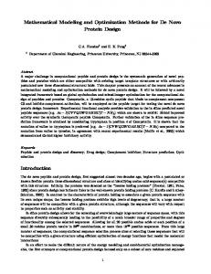
INTRODUCTION TIG welding is an arc-welding process that produces coalescence of metals by heating them with an arc between a non-consumable tungsten electrode and the base metal [1]. Many delicate components in aircraft and nuclear reactors are TIG welded due to its reliability. Basically, TIG weld quality is strongly characterized by the weld pool geometry as shown in Figure 1. This is because the weld pool geometry plays an important role in determining the mechanical properties of the weld [2]. TIG welding is a highly non-linear, strongly coupled, multivariable process [3, 4, 5]. The weld pool geometry and, hence, the quality of TIG welded joints are greatly dependent on the selection of input control variables such as welding speed (V), welding current (I), shielding gas flow rate (F) and gap distance (G). Therefore, in the TIG welding, engineers often face with the problem of selecting appropriate and optimum combinations of input control variables for the required weld pool quality. In this work, nonlinear and multi-objective mathematical models are developed for the selection of the optimum processes parameters. First, the upper and lower limits of the input control variables are obtained and the U. Esme, Technical Education Faculty, Department of Mechanical Education, Mersin University, Tarsus; A. Kokangul, Department of Mechanical and Industrial Engineering, Cukurova University, Adana; M. Bayramoglu, N. Geren, Department of Mechanical Engineering, Cukurova University, Adana, Turkey

METALURGIJA 48 (2009) 2, 109-112

Figure 1. Weld pool geometry

effect of the input control variables on the weld pool quality parameters is determined. Then, the mathematical relationships between the input control variables and weld pool quality parameters are obtained. These relationships are considered as objective functions in the mathematical models. To the best of our knowledge the optimization problem of the TIG welding using nonlinear and multi-objective mathematical models has not been investigated previously and applied on real life case study like in this work.

A SYSTEMATIC APPROACH Development of a systematic approach is required to obtain optimum combinations of input control variables for the required weld pool quality system. This approach includes the following steps. I) Identify the process control variables and their upper and lower limits, 109

U. ESME et al.: MATHEMATICAL MODELING FOR PREDICTION AND OPTIMIZATION OF TIG WELDING POOL...

where S 1+ and S 2+ represent the positive components, S 1and S 2- represent the negative components and S 1+ , S 1- , S 2+ , S 2- ³ 0.

II) Identify the quality parameters, III) Construct mathematical models, IV) Develop a design matrix , V) Conduct experiments, VI) Obtain mathematical relationships, VII) Apply the constructed models.

Step 4. It is aimed to approach TLopt and HAZopt with the same percent as closely as possible in which case the objective function is not measured in a common unit. To ensure this the following constraint is added:

Input process control variables The independently controllable parameters affecting weld pool geometry and the quality of the weld pool V, I, F and G were selected as input control variables.

(HAZopt) S 1+ = (TLopt )S 2-

(10)

The objective function is:

It is possible to present the quality of welding geometry with the TL, P, AP, HAZ, UW and UH. These parameters are important weld quality parameters and all of them are considered in this study.

(11) Min S 1+ - S 2The optimization problem aims to find the optimal value of the multi-objective function (11) under (2-5), (8), (9) and (10) constraints. By the same way, for each of the other combination of objectives a multi-objective mathematical model can be constructed. In order to apply the constructed optimization models, a design matrix must be developed.

Constructing mathematical models

Development of the design matrix

The engineer would like to determine the level of input control variables according to the only one weld pool quality parameter such as maximizing TL. In the first nonlinear model, as seen below, let us maximize TL under the upper and lover limit of the input control variables indicated with “U” and “L” indices, respectively. Maximizing TL (1) Constraints: (2) VL £V£VU (3) IL £I£IU (4) FL £F£FU (5) GL £G£GU By the same way four models are constructed for the rest of the weld pool quality parameters. In same cases the engineer would like to consider a few objectives simultaneously. Let’s in the next model maximize TL and minimize HAZ simultaneously. To construct the necessary multi-objective model the following procedures are applied: Step 1. Find the maximum level of TL (TLopt) under the (2-5) constraints. Step 2. Find the minimum level of HAZ (HAZopt) under the (2-5) constraints. Step 3. In addition to the (2-5) constraints add the following constraints. (6) TL³TLopt (7) HAZ£HAZopt It is not expected that all of these constraints be satisfied simultaneously. The right hand sides are variable constraints with flexibility, which are managerial goals to be approached as closely as possible. To this end, constraints (6) and (7) are equated as follows: (8) TL+ S 1+ - S 1- = TLopt

The design matrix should be depending on the upper and the lower limits of the predetermined input control variables. The selected design matrix is a four-level, four-factor, central composite rotatable response surface design consisting of 90 sets of design matrix. It comprises response surface design (RSD) plus 18 center points. All welding variables at their intermediate level (0) constitute the center points. The upper limit of a variable was coded as +2 and the lower limit as –2. The coded values for intermediate values were calculated from the rotatable central composite design of Design Expert 6.0 as given in Table 1.

Weld pool quality parameters

HAZ + S 2+ - S 2- = HAZopt 110

(9)

Table 1. Lower and upper limits of factors Welding parameters

Min. value (-2)

Max. value (+2)

Low level (-1)

High level (+1)

Travel speed, V (mm/s)

1,07

3,55

1,69

2,93

Current, I(A)

20

150

52

117

Gas flow rate, F(l/min)

8

12

9

11

Gap distance, G(mm)

1

4

1.75

3.25

For each of determined combination of the input control variables (V, I, F and G) perform the TIG welding and determine the value of the quality parameters using conducting experiments.

Conducting experiments The experimental set up was designed and constructed to control the linear movement of the torch along the weld pad center line. The experiments were conducted according to the design matrix at random order to avoid systematic errors infiltrating the system. METALURGIJA 48 (2009) 2, 109-112

U. ESME et al.: MATHEMATICAL MODELING FOR PREDICTION AND OPTIMIZATION OF TIG WELDING POOL...

Weld pools were laid on the joint to join thin stainless steel plate with the experimental setup. AISI type 304 stainless steel plates of 1,2 mm thicknesses were used as a workpiece material. The specimens were joined using a single pass welding with AWS A 5.12-80 EW Th-2 thoriated (red color code) tungsten electrode with 1,6 mm diameter and argon as shielding gas. The chemical compositions of the used work-piece material obtained from spectra analysis are given in Table 2. The welded joints were sectioned to produce specimens for examining the quality parameters (UW, UH, P and AP) of weld pool shape in the welded specimens. Table 2. Composition (%) of used AISI 304 steel C

Mn

P

S

Si

Cr

Ni

Cu

0,08

2,0

0,04

0,03

1,0

19

10,5

0,02

These specimens were prepared by the usual metallurgical polishing methods and etched with Marble’s etching reagent (CuSO4 + HCl + H2SO4). Macrographs were then taken for each cross section using stereo microscope with 50X lens. In macro examinations of the specimens, MOTIC stereo microscope with image capture device mounted on top of the lens section of the microscope was used. The weld pool profile was outlined by using Image-pro Plus 4.5 and NIH ImageJ software. The spatial calibrations were made on the macrographs before the measurement. The line drawings of the pool profiles were then used to take measurements on UW, UH, P, AP and HAZ. Tensile load values were recorded from tensile testing of the specimens prepared in accordance with the EN 895 Standard. Tensile test specimens were taken from the weld bead according to the transverse tensile test method. Tensile test specimens were prepared in such a way that the weld zones were centered in the gage length. At the same time, heat affected zone was placed in the gage length perpendicular to the weld.

Mathematical relationships The suitable mathematical relationship such as a second-degree response surface quadratic model (seen be-

low) should be selected for each of the process quality parameters according to the experimental results. Y = b0 + b1V + b2I + b3F + b4G + b11V2 + b22I2 + b33F2 + b44G2 + b12VI + b13VF +b14VG + b23IF + b24IG + b34FG where “b” values are the coefficients of the models. These values can be calculated using Design Expert 6.0 software.

Application of the systematic approach The working range is decided upon by inspecting the weld pool for a smooth appearance without any visible defects such as surface porosity and undercut. The combinations of the input control experimental runs for each of the 90 combination of the input control variables, and for each of the combination value of the weld quality parameters are obtained and used. Thus, these will allow to the estimate the effects of the input control variables on the weld pool quality parameters mathematically. The best mathematical relationship obtained for weld pool quality parameters (HAZ, TL, UW, P, UH and AP) are represented in Table 3. The obtained mathematical relationships were tested individually using ANOVA analysis. The test results for HAZ are as follows: The value of the multiple coefficient of R2 is obtained as 0,92, which means that the explanatory variables explain 92 % of the variability in response variable. Adjusted R-square is generally the best indicator of the fit quality and it is obtained as 0,90. The test results of the obtained mathematical relationships show that the model fits well to the observations. The constructed nonlinear mathematical model (maximizing TL (1) under 2-5 constraints) can be constructed as follows using the determined upper and lower limits of the input control variables (as seen in Figure 1). Maximizing TL, 1,07£V£3,55

(12)

20£I£150

(13)

8£F£12

(14)

1£G£4

(15)

Table 3. The mathematical relationships for process quality parameters HAZ=4,2573-2,2532V+0,0781I+0,027766F + 0,1975G+0,3520V2-0,000124I2 – 0,001384F2-0,021331G2-0,006771VI– 0,001035VF+0,000108VG-0,000127IF+0,001067IG-0,004653FG TL=9,80665+238,03487V+8,1026I+25,05345F+4,03510G-75,10057V2-0,039932I2-1,78092F2-7,09131G2-0,059916VI+3,34043VF +0,73102VG-0,041339IF+0,04571IG+1,17361FG UW=3,30265+0,44806V+0,089617I+0,20048F+0,074331G-0,21720V2–0,000128I2-0,015592F2–0,004656G2-0,011222VI+0,0080 71VF-0,027623VG+0,000131IF+ 0,000763IG+0,010625FG UH=0,083160-0,14708V+0,004271I+0,026577F-0,039542G+0,029239V2–0,000001237I2-0,00090246F2+0,0029819G2-0,000767 36VI-0,0011008VF+0,00603239VG-0,00008549IF– 0,0001254IG+0,001736FG P=0,64397+0,066087V+0,006967I+0,018256F+0,087894G-0,019590V2–0,000039I2-0,000551F2-0,014174G2+0,000502VI-0,003 323VF-0,020984VG+0,000052IF+ 0,000333IG-0,001458FG AP=3,94256-0,19505V+0,084155I+0,21323F+0,46969G-0,019710V2–0,000126I2-0,012660F2-0,10079G20,013011VI-0,020638VF-0,048323VG+0,0005887IF+0,000453IG +0,012111FG

METALURGIJA 48 (2009) 2, 109-112

111

U. ESME et al.: MATHEMATICAL MODELING FOR PREDICTION AND OPTIMIZATION OF TIG WELDING POOL...

Table 4. Results of mathematical models Objective

Input process control variables F I/min

Optimal Values

V mm/s

I A

G mm

TL N

HAZ mm

UW mm

UH mm

P mm

AP mm2

Max TL

1,73

96,59

Min HAZ

3,41

20

8

1

12963,2

6,93

10,02

0,27

1,26

9,67

12

1

8666,5

1,92

3,92

0,04

0,81

3,22

Min UW

3,55

20

12

1

8331,0

1,93

3,75

Min UH

2,81

20

8

2,04

9721,1

2,21

4,95

0,05

0,79

3,11

0,02

0,86

4,47

Max P

1,07

117,3

12

3,07

11688,6

9,42

12,08

0,30

1,34

11,43

Max AP

1,07

150

12

1

11036,2

10,27

13,08

0,39

1,21

12,86

Multi objective nonlinear models Max TL Min HAZ

2,41

20

9,41

1

10375,6

2,30

5,15

0,05

0,91

4,81

Max TL Min HAZ,UW

2,72

20

12

1

9901,0

2,09

4,64

0,03

0,88

4,03

Max TL Min HAZ, UW, UH

2,99

20

12

1,17

9488,6

2

4,40

0,03

0,85

3,70

Max TL, P Min HAZ, UW, UH,

2,69

20

8

1,62

9969,5

2,22

5,03

0,03

0,88

4,61

Max TL, P, AP Min HAZ,UW, UH,

2,49

21,02

8

2,19

10162,5

2,45

5,31

0,03

0,90

4,94

This kind of mathematical models can be solved using optimization software such as LINGO 8.0, MATLAB 7.0. The obtained global optimal solution is given in Table 4. In addition, by the same way for the other quality parameters five nonlinear models are constructed and solved under the same constraints (12-15). Their results are shown in Table 4. In case of the engineer aims to maximize TL and minimize HAZ simultaneously under the same constraints, the constructed multi-objective mathematical model (minimizing Eq. 11 under the constraints of 2-5, 8, 9 and 10 ) will be as follows: As seen in table 4, the TLopt is obtained as 12963,21 N, and HAZopt as 1,92 mm. Therefore, the objective function (11) and the constraint 8, 9 and 10 will be as follows: (16) Min S 1+ + S 2-

TIG welding process parameters. The mathematical relationships between input control variables and weld pool quality parameters are obtained using the results of experiments. Six nonlinear and five multi-objective mathematical models are constructed and solved under the predetermined limits of the input control variables using the obtained mathematical relationships as objective functions. This developed systematic approach can also be adopted for other type of arc welding processes.

TL+ S 1+ - S 1- =12963,21 N

(17)

[2]

HAZ+ S 2+ - S 2- =1,92 mm

(18)

+ 1

1,92 S =12963,21 S

2

(19)

For this multi-objective mathematical model the global optimal solution is given in Table 4. By the same way as seen in Table 4, five multi objective models are constructed and solved. When the engineer considers more than one objective, then the optimum values will be decreased compared to the optimal values obtained using one objective model. The engineer can then easily find the optimal level of input control variables using the results given in Table 4 according to the objectives.

REFERENCES [1]

[3] [4] [5]

S.C. Juang, Y.S. Tarng, H.R. Lii, A comparison between the back propagation and counter-propagation networks in the modeling of the TIG welding process, J. Mater. Process. Technol. 75 (1998) 54–62. S.C. Juang, Y.S. Tarng, Process parameter selection for optimizing the weld pool geometry in the tungsten inert gas welding of stainless steel, J. Mater. Process. Technol., 122 (2002) 33–37. Y.M. Zhang, R. Kovacevic, L. Li, Characterization and real-time measurement of geometrical appearance of the weld pool, Int. J.Mach. Tools Manuf., 36 (7) (1996) 799–816. Y.S. Tarng, H.L. Tsai, S.S. Yeh, Modeling, optimization and classification of weld quality in TIG welding, Int. J. Mach. Tools Manuf. 39 (9) (1999) 1427–1438. H.B. Cary, Modern Welding Technology, Prentice-Hall, Englewood Cliffs, NJ, 1989.

Note: The responsible translator for English Language is U. Esme, Technical Education Faculty, Mersin University, Tarsus, Turkey.

CONCLUSIONS A systematic approach has been developed and employed in this study for the optimization problem of the 112

METALURGIJA 48 (2009) 2, 109-112